Improving Hardware in LUT-Based Mealy FSMs

Abstract

The main contribution of this paper is a novel design method reducing the number of look-up table (LUT) elements in the circuits of three-block Mealy finite-state machines (FSMs). The proposed method is based on using codes of collections of outputs (COs) for representing both FSM state variables and outputs. The interstate transitions are represented by output collections generated during two adjacent cycles of FSM operation. To avoid doubling the number of variables encoding of COs, two registers are used. The first register keeps a code of CO produced in the current cycle of operation; the code of a CO produced in the previous cycle is kept in the second register. There is given a synthesis example with applying the proposed method. The results of the research are shown. The research is conducted using the CAD tool Vivado by Xilinx. The experiments prove that the proposed approach allows reducing the hardware compared with such known methods as auto and one-hot of Vivado, and JEDI. Additionally, the proposed approach gives better results than a method based on the simultaneous replacement of inputs and encoding of COs. Compared to circuits of the three-block FSMs, the LUT counts are reduced by an average of 7.21% without significant reduction in the performance. Our approach loses in terms of power consumption (on average 9.62%) and power–time products (on average 10.44%). The gain in LUT counts and area–time products increases with the increase in the numbers of FSM states and inputs.

1. Introduction

Nowadays, it is characteristic the fact that numerous digital systems are widely used in the daily life of human society [1,2]. Among other digital equipment, contemporary systems include a lot of various sequential devices [3]. The law of operation of a sequential device can be described by the model of the Mealy finite state machine (FSM) [4]. This model is used, for example, to set the behavior of (1) control devices [5,6]; (2) serial communication and display protocols [7]; (3) various software tools of embedded systems [8]; (4) control-dominated systems [9]; (5) different systems in robotics [10] and so on. This analysis led to the choice of the Mealy FSM model in our recent research.

The process of FSM-based design is connected with raising some optimization problems [5,7]. As a rule, the following characteristics of FSM circuits should be improved: the occupied chip area, the time of cycle (the maximum operating frequency) and the consumed power. The approaches used for reducing these values depend strongly on the peculiarities of logic elements used for implementing the FSM circuits. Changing the type of logic elements leads to the necessity for changing the optimization approaches. This is the reason for the continuous interest in developing new design methods aiming at the optimization of FSM circuits. These characteristics are interrelated. For example, the area reduction leads to reducing the power consumption [11,12]. Due to the great importance of the area reduction, we devote our article to this problem.

The area reduction of LUT-based FSM circuits may be achieved using the methods of structural decomposition (SD) [13]. In this case, an FSM circuit is represented as a composition of two to four large logical blocks. These blocks have unique systems of input variables and output functions distinguishing them from other circuit blocks [14]. In this article, we propose an alternative to the method discussed in [15]. The original method [15] is reduced to joint applying the replacement of inputs and encoding of collections of outputs (COs) [5]. Applying these methods is connected with generating two additional systems of functions. Implementing circuits for these additional systems requires using some chip resources. In this article, we propose to use the same variables both for encoding the COs and for the replacement of the FSM inputs. This leads to the elimination of a block generating the additional variables replacing the FSM inputs. As a result, this reduces the number of LUTs compared to this number for the equivalent circuit based on the approach of [15].

The main contribution of this paper is a novel design method which allows diminishing the LUT count (the number of LUTs) in the circuits of three-level Mealy FSMs with the joint use of two methods of structural decomposition. The proposed method is based on using the same additional variables as inputs of logic blocks generating both input memory functions (IMFs) and FSM outputs. Due to this, there is eliminated a block replacing FSM inputs inherent in the method [15]. The main purpose of the proposed method is to reduce the LUT count in the FSM circuit without significantly impairing the FSM performance.

The further text of the paper is organized in the following order. The second section contains basic information related to LUT-based Mealy FSMs. The third section discusses the necessary elements of the state of the art. In this section, we provide a critical analysis of existing synthesis methods and show the need for their improvement. The fourth section highlights the main idea of the proposed method. An example of synthesis is presented and analyzed in the fifth section. The sixth section includes the results of experiments and their analysis. A brief conclusion ends the paper.

2. Basics of LUT-Based Mealy FSM Design

In this section, we show the basics of designing FSMs circuits using internal resources of FPGAs. Here, we introduce the main notation used in the rest of the text and show the features of the logic elements used. At last, we introduce the simplest structural diagram of a Mealy FSM circuit implemented with LUTs and programmable flip-flops.

For a better understanding of the material of the article by readers, we introduce Table 1. This table shows the main sets of variables and the notation adopted in our article.

Table 1. The main notation used in the article.

$A=\{a_1,\dots ,a_M\}$	The set of FSM internal states having M elements.
$B=\{b_1,\dots ,b_J\}$	The set of additional variables replacing FSM inputs having J elements where $J\ll L$.
I	The number of LUT inputs.
$K\left(a_m\right)$	The binary code of state $a_m\in A$.
$K\left(Y_q\right)$	The binary code of collection of outputs $Y_q\subseteq Y$ with $R_q=\lceil lo{g}_{2}Q\rceil$ bits.
$NA\left({\varphi }_k\right)$	The number of literals in a function ${\varphi }_k\in \Phi \cup Y$.
$P_g=<Y_i,Y_j>$	A pair of collections of outputs replacing a pair <state, input>.
$\Phi =\{D_1,\dots ,D_R\}$	The set of FSM input memory functions having R elements.
Q	The number of collections of outputs $Y_q\subseteq Y$.
R	The number of bits in the codes $K\left(a_m\right)$ determined as $R=\lceil lo{g}_{2}M\rceil$.
$T=\{T_1,\dots ,T_R\}$	The set of state variables for creating the codes $K\left(a_m\right)$ with R bits.
$V=\{v_1,\dots ,v_{RQ}\}$	The set of additional variables encoding collections of outputs from the current cycle of FSM operation having RQ bits.
$X=\{x_1,\dots ,x_L\}$	The set of FSM inputs having L elements.
$Y=\{y_1,\dots ,y_N\}$	The set of FSM outputs having N elements.
$Z=\{z_1,\dots ,z_{RQ}\}$	The set of additional variables encoding collections of outputs from the previous cycle of FSM operation having RQ bits.

To start the designing process, it is necessary to set the law of the FSM behavior. For this, various mathematical apparatuses can be used [1]. Two methods are most commonly used for this purpose: (1) a state transition graph (STG) and (2) a state transition table (STT) [16]. We use both forms in this article. These forms are used to derive systems of Boolean functions (SBFs) defining dependencies between FSM outputs and input memory functions on the one hand, and FSM inputs and state variables on the other hand. These SBFs are used to design FSM logic circuits [16].

The FSM inputs create a set $X=\{x_1,\dots ,x_L\}$, the FSM outputs form a set $Y=\{y_1,\dots ,y_N\}$. The inputs determine transitions between FSM states combined into a set $A=\{a_1,\dots ,a_M\}$. To synthesize an FSM circuit, the states $a_m\in A$ are represented by binary codes $K\left(a_m\right)$ having R bits. The states are encoded using state variables from the set $T=\{T_1,\dots ,T_R\}$. The r-th bit of a state code is represented by an internal state variable $T_r\in T$. The minimum value of R is calculated using the following formula:

$$R=\lceil lo{g}_{2}M\rceil .$$

(1)

The Formula (1) determines so-called maximum state codes [17]. A special register $RG$ is entered into the FSM circuit as a memory of the state codes [5]. In the case of FPGA-based FSMs, the $RG$ is implemented using D flip-flops [17,18]. The content of $RG$ is determined by the input memory functions combined into a set $\Phi =\{D_1,\dots ,D_R\}$. The IMFs are inputs of $RG$ showing a direction of a particular interstate transition.

The SBFs that make it possible to synthesize an FSM circuit can be formed using a direct structure table (DST) [5]. A DST is constructed on the base of either the initial STT or STG. An STT includes the following columns [16]: a current state $a_m$ (a state for the current instant); a state of transition $a_T$ (a state for the next instant); an input signal $X_h$ determining the transition from $a_m$ into $a_T$ (it is a certain conjunction of inputs); a collection of outputs (CO) $Y_h$ formed during the transition $<a_m,a_T>$; and the numbers of transitions are shown in the column h. There are H lines in an STT. A DST includes all these columns and three additional columns. These additional columns are [5] the current state code $K\left(a_m\right)$, the next state code $K\left(a_T\right)$, and IMFs ${\Phi }_h\subseteq \Phi$, which allows loading the next state code into $RG$.

Using a DST, the following SBFs are constructed:

$$\Phi =\Phi (T,X);$$

(2)

$$Y=Y(T,X).$$

(3)

The SBF (2) corresponds to the FSM transition function [5] that specifies the dependence of the states of transition on the current states and input variables. The SBF (2) represents rules of generating IMFs necessary to load a next state code into the $RG$. The SBF (3) corresponds to the FSM output function [5] that specifies the dependence of the FSM outputs on the current states and input variables. The SBF (3) represents rules of generating FSM outputs during each interstate transition. The SBFs (2) and (3) are the basis for the synthesis of FSM $U_1$, whose structural diagram is shown in Figure 1.

Figure 1. Structural diagram of FSM $U_1$.

In Figure 1, the $BlockY\Phi$ implements the SBFs (2) and (3). The $RG$ includes R flip-flops. The pulse Res loads the code of the initial state $a_1\in A$ into $RG$. Very often, there are only zeros in the code $K\left(a_1\right)$ [18]. The synchronization pulse Clk allows loading state codes into $RG$.

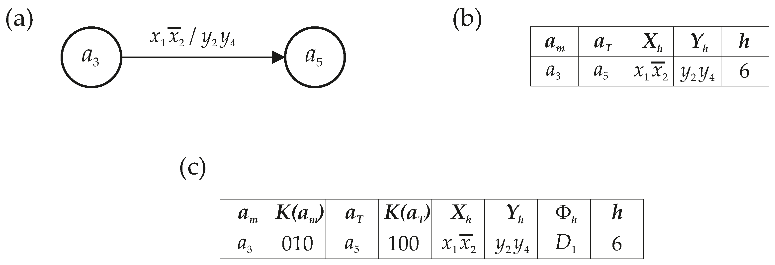
Consider a transition between the states $a_3$ and $a_5$ of some Mealy FSM. Let it be the transition with $h=6$. The transition is represented using fragments of three equivalent forms: an STG, an STT and a DST (Figure 2).

Figure 2. Equivalent fragments of STG (a), STT (b) and DST (c).

As follows from Figure 2a, the transition $<a_3,a_5>$ is caused by the input signal $X_6=x_1\overline{x_2}$. The transition is accompanied by the producing of a CO $Y_6=\{y_2,y_4\}$. Row 6 of the STT (Figure 2b) is a sequence of characters corresponding to the fragment of STG (Figure 2a). If, for example, there is $M=7$, then using (1) gives $R=3$ and two sets: $T=\{T_1,T_2,T_3\}$ and $\Phi =\{D_1,D_2,D_3\}$. For a trivial state assignment [5], there are the codes $K\left(a_3\right)=010$ and $K\left(a_5\right)=100$. These codes and IMF $D_1$ are written in the sixth line of DST (Figure 2c). This line determines a product term $F_6=\overline{T_1}{T}_2\overline{T_3}{x}_1\overline{x_2}$. This term is a part of the sum of products (SOPs) of Boolean functions $D_1\in \Phi$ and $y_2,y_4\in Y$. All other terms of SOPs for (2) and (3) are obtained in the same way [5].

In this paper, we discuss a case of implementing SBFs (2) and (3) using configurable logic blocks (CLBs) and other internal resources of FPGA chips [19]. To form an FSM circuit, the CLBs are connected using a programmable routing matrix [17,20]. In this paper, we consider CLBs, including LUTs, multiplexers and programmable flip-flops. Similar to the notation used in the paper [21], we use a symbol I–LUT to denote a single-output LUT having I inputs. Such a LUT can implement an arbitrary Boolean function having up to I arguments. The analysis of the FPGA market shows that AMD Xilinx dominates this market [19]. Due to it, we focus our current research on the solutions of Xilinx. These solutions are very popular at present for the implementation of various projects. This fact is confirmed by the analysis of the literature [22,23,24,25,26,27,28].

If the number of arguments of a Boolean function is greater than I, then the corresponding circuit can be implemented with the help of the functional decomposition (FD) [29,30,31,32]. In this case, the resulting circuits are, as a rule, multi-level. Additionally, they are characterized by very complex systems of “spaghetti-type” interconnections [13].

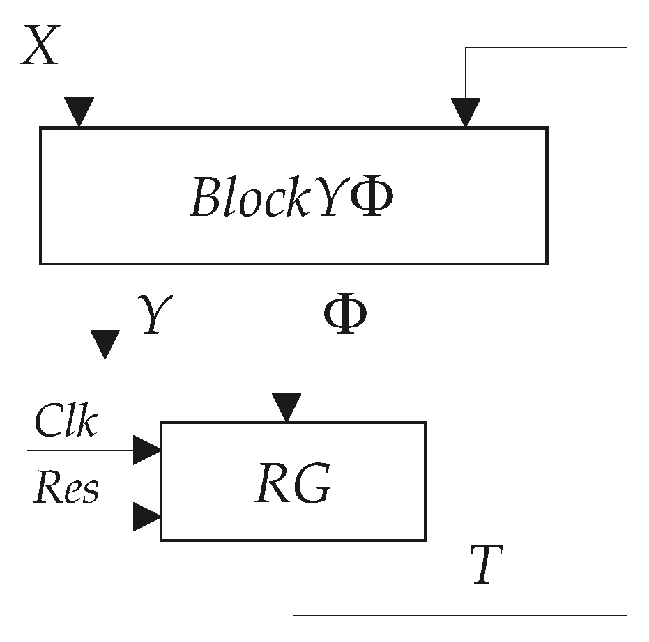
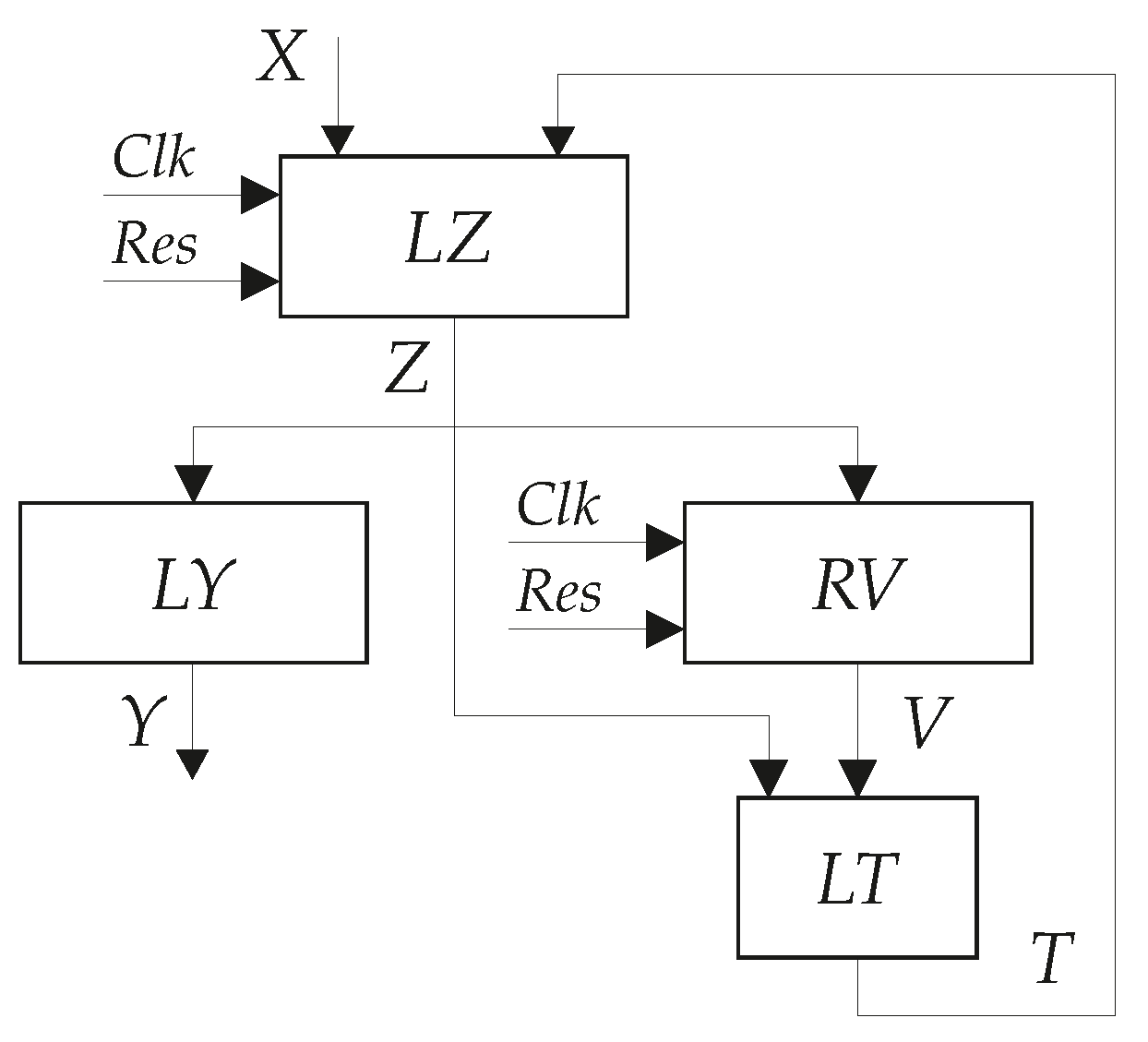
In LUT-based FSMs, the $RG$ is hidden and distributed among CLBs generating IMFs. Due to it, the logic circuit of LUT-based FSM $U_1$ consists of two logic blocks (Figure 3).

Figure 3. Structural diagram of LUT-based FSM $U_1$.

In Mealy FSM $U_1$, the block $LSV$ consists of CLBs generating SBF (2). The state code is kept in the hidden register $RG$. Due to it, the pulses Res and Clk enter the block $LSV$. The outputs $y_n\in Y$ are generated by the block $LY$. This block does not include flip-flops; it implements SBF (3).

3. Related Work

This section provides a brief analysis of basic methods used for reducing the number of LUTs in FSM circuits. We show that this problem can be solved using either a certain state assignment or various methods of functional and structural decomposition. We show the disadvantages inherent in the methods from these three groups. The method proposed in this paper belongs to the group of structural decomposition methods.

Under certain conditions, there is only one level of LUTs in the circuit of $U_1$. To implement a single-level circuit, each function ${\varphi }_k\in \Phi \cup Y$ should depend on no more than I arguments. However, there are up to six address inputs in the present-day LUTs [19,33,34]. To balance the area-spatial-power characteristics of a LUT, it is necessary that the number of inputs does not exceed six [35]. Nevertheless, the total number of inputs and state variables of an FSM can significantly exceed the value of I. This leads to an imbalance between a very large number of FSM inputs, outputs and states, on the one hand, and a very small number of LUT inputs, on the other hand. To reduce the negative impact of this imbalance, it is necessary to improve the design methods of FPGA-based FSMs.

The required chip area can be reduced due to the optimizing of the system of interconnections for a particular circuit. Improving interconnections can reduce the power consumption because more than 70% of the power consumption is due to the interconnections [36]. Additionally, the interconnections are responsible for the value of maximum operating frequency of a resulting FSM circuit. As it is shown in [36], the complexity of the interconnection system is beginning to have an increasing negative impact on the propagation time of signals in the FSM circuits. As follows from [15], the regularization of interconnections results in reducing both the time and power consumption. To regularize the interconnection system, it is necessary to use the structural decomposition methods [13,37].

If the condition

$$NA\left({\varphi }_k\right)\le I$$

(4)

holds for each function ${\varphi }_k\in \Phi \cup Y$, then there are $L+R$ I-LUTs in a single-level circuit of the corresponding FSM $U_1$. However, if the condition (4) does not hold for some functions ${\varphi }_k\in \Phi \cup Y$, then it becomes impossible to represent such an FSM with a single level of LUTs. To improve the characteristics of multi-level circuits, various methods can be applied.

A significant number of optimization methods aimed at FPGA-based FSMs can be found in the literature [13,17,18,21,32,38,39,40,41]. As a rule, these methods can improve the value of one of the characteristics of the FSM circuit [39,40]. Additionally, there are methods which simultaneously reduce the values of two characteristics (area and power consumption, or area and performance). In our current paper, a method is proposed which aims at reducing the LUT count of three-block circuits of Mealy FSMs [15].

The values of $NA\left({\varphi }_k\right)$ can be reduced with the help of a proper state assignment [41,42,43]. The number of FSM state memory elements is in the range from $R=\lceil lo{g}_{2}M\rceil$ to $R=M$. The upper limit of this amount ($R=M$) corresponds to a one-hot state assignment. Both of these extreme approaches can be found in many CAD tools, such as SIS [44], ABC [32,45] or Sinthagate [46]. The manufacturers of FPGA chips also have their tools for implementing the technology mapping of LUT-based circuits. Examples of such systems are Vivado [47], Vitis [48], and Quartus [49]. The first two CAD systems were developed by AMD Xilinx, and the third one is a product of Intel (Altera).

It is impossible to specify the approach that is optimal for any FSM. For example, in [50], there is given the comparison of the synthesis results for FSM circuits based on state codes with $R=\lceil lo{g}_{2}M\rceil$ and one-hot state codes. Note that both of these approaches are widely used in most modern CAD tools. As follows from the comparison, the one-hot codes are the best choice for FSMs with more than 16 states. However, in addition to the value of R, the number of input variables also has a very strong influence on the characteristics of LUT-based FSM circuits. For example, the experiments [51] definitely show the following: if the number of FSM inputs exceeds 10, then it is better to use the codes with a minimum number of bits.

As follows from this analysis, it is necessary to check which method leads to the best results for a specific combination of characteristics of a particular FSM. In this paper, we compared the results produced by our new approach with the characteristics of FSM circuits produced using the algorithm JEDI [44], and the methods auto ($R=\lceil lo{g}_{2}M\rceil$) and one-hot ($R=M$) of Vivado [47] by Xilinx [19]. Our choice of JEDI is due to the fact that it is considered one of the best deterministic methods of the state encoding [44].

If condition (4) is violated, then various methods of functional decomposition should be applied to implement an FSM circuit [29,39]. All these methods are based on splitting the original SOP into sub-SOPs for which the number of arguments does not exceed the number of LUT inputs. Each sub-SOP corresponds to a partial function which differs from the initial function ${\varphi }_k\in \Phi \cup Y$ [39]. This splitting should be executed in a way that increases the number of logic levels of the final FSM circuit as little as possible [29]. Practically, the methods of FD are included in each academic and industrial CAD tool dealing with the LUT-based design. The main disadvantage of FD-based methods: they produce the FSM circuits with spaghetti-type interconnections [13]. It is known that such circuits lose in all three main characteristics to their counterparts with a regular interconnection system [52].

The methods of structural decomposition [13] are an alternative to the methods of FD. The main idea of these methods is the elimination of the direct connection between FSM inputs and state variables, on the one hand, and FSM outputs and IMFs, on the other hand. In the case of SD, an FSM circuit is represented as a composition of unique logic blocks. This leads to an increase in the number of implemented functions, but these partial functions are much simpler than functions (2) and (3). The analysis of these methods can be found, for example, in [13].

The first known methods of SD are the replacement of inputs (RI) and the encoding of the collections of outputs (ECO). They were proposed in the mid-twentieth century by M. Wilkes for the optimization of microprogram control units [53]. In [15], we proposed the joint use of these methods for the optimization of LUT-based Mealy FSMs’ circuits. Let us briefly describe these two methods.

In the case of $RI$, the set $X=\{x_1,\dots ,x_L\}$ is replaced by a set of additional variables $B=\{b_1,\dots ,b_J\}$, where $J\ll L$. The replaced inputs are represented by an SBF

$$B=B(T,X).$$

(5)

Each function of (5) represents a multiplexor. Its control inputs are connected with the state variables, and the data inputs are connected with the replaced inputs. In the case of CLB-based solutions, these multiplexors are implemented using LUTs and dedicated multiplexors [54].

There are Q different COs. Each collection $Y_q\subseteq Y$ includes FSM outputs generated during a particular interstate transition. As a rule, the condition $Q<H$ holds, where H is a number of interstate transitions. The COs are encoded by binary codes $K\left(Y_q\right)$. The bits of $K\left(Y_q\right)$ are represented by elements of an additional set $Z=\{z_1,\dots ,z_{RQ}\}$. The cardinality number of the set Z is determined as

$$R=\lceil lo{g}_{2}Q\rceil .$$

(6)

To encode COs, two additional SBFs should be constructed:

$$Z=Z(T,X);$$

(7)

$$Y=Y\left(Z\right).$$

(8)

The SBFs (7) and (8) are implemented using LUTs. Obviously, the system (8) is represented by $R_Q$ decoders.

Combining the methods of $RI$ and $ECO$ leads to the replacement of both SBFs (2) and (7). Now, the following SBFs should be constructed:

$$\Phi =\Phi (T,B);$$

(9)

$$Z=Z(T,B).$$

(10)

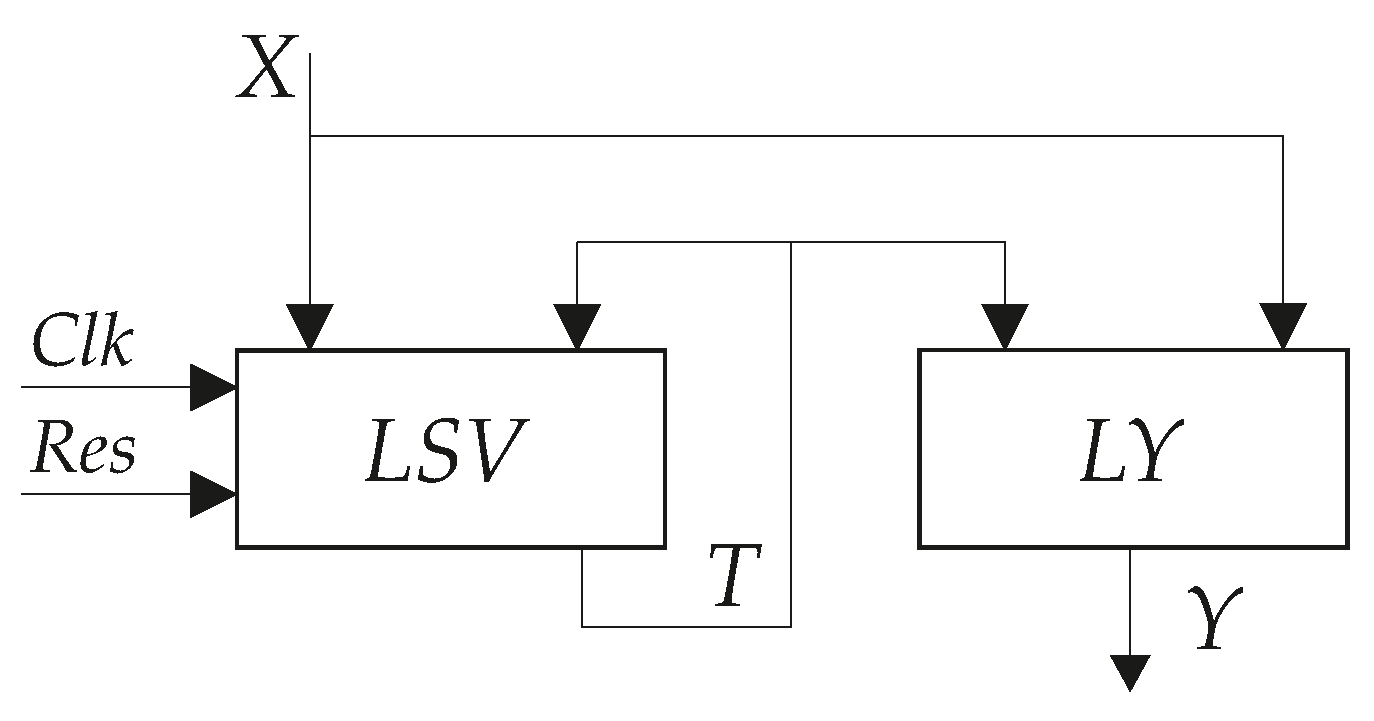
The SBFs (5), (8)–(10) determine a structural diagram of FSM $U_2$ (Figure 4).

Figure 4. Structural diagram of Mealy FSM $U_2$.

In FSM $U_2$, a $BlockB$ implements SBF (5). The variables $b_j\in B$ enter a $BlockZ\Phi$ implementing SBFs (9) and (10). The IMFs $D_r\in \Phi$ enter the state code register $RG$. The variables $z_r\in Z$ are transformed into the FSM outputs $y_n\in Y$ by a $BlockY$.

In LUT-based FSMs, these blocks are implemented using the internal resources of CLBs, inter-slice interconnections, programmable input–outputs and synchronization tree buffers [54]. In [15], we compared the characteristics of $U_1$- and $U_2$-based FSMs. The research results obtained in [15] show that the joint use of $RI$ and $ECO$ allows to significantly reduce the LUT counts in FSM circuits.

To optimize an FSM circuit, we propose using the variables $z_r\in Z$ for generating both FSM outputs and IMFs. To make it possible, we propose to use codes of COs generated in two neighboring instances of the FSM discrete time.

4. Main Idea of the Proposed Method

The analysis of FSM $U_2$ (Figure 4) allows finding its shortcomings. The main drawback of $U_2$ is the need to form two systems of additional variables. One of them serves to replace the inputs $x_l\in X$, and the second system is used to encode the collections of outputs. These systems are represented by SBFs (5) and (10), respectively. To implement these systems, it is necessary to use some internal resources of FPGA chip. The amount of resources used can be reduced by using the same additional variables to implement both input memory functions and FSM outputs. In our article, there is proposed such an approach. Our analysis of the extensive literature shows that so far, there has been no such a method. Due to it, the proposed method has an undeniable scientific novelty.

Our method is based on using the codes of collections of FSM outputs for generating IMFs $D_r\in \Phi$. Consider Figure 5 where this idea is illustrated.

Figure 5. Illustration of the main idea of proposed method.

A subgraph of some STG is shown in Figure 5. The generator of pulses Clk sets the course of discrete time $t(t=0,1,2,\dots )$. Three instances of time are shown in Figure 5. In the instant of time t, the FSM is in the state $a\left(t\right)=a_4$. The transition from $a_3$ into $a_4$ is accompanied by producing a CO $Y_5$. So, the following relation takes place: $Y_q\left(t\right)=Y_5$. From STG (Figure 5), we can find that $a(t+1)=a_5$ and $Y_q(t+1)=Y_3$. So, the transition $<a_4,a_5>$ corresponds to a pair of COs $<Y_5,Y_3>$. This transition is caused by an input $x_2\in X$. So, the pair $<a_4,x_2>$ also corresponds to a pair of COs $<Y_5,Y_3>$. This means that IMFs can be represented using only codes of COs.

In FSM $U_2$, the SOPs of functions $D_r\in \Phi$ include product terms $F_h$ determined as

$$F_h=A_m\wedge B_h.$$

(11)

In (11), the symbol $A_m$ stands for a conjunction of the state variables corresponding to the code of a current state $a_m$ written in the h-th row of DST; the symbol $B_h$ stands for a conjunction of additional variables replacing the input signal $X_h$ written in the h-th row of DST ($h\in \{1,\dots ,H\}$). If a pair $<a_m,X_h>$ determines the h-th transition of an FSM, then we propose to replace it by a pair of COs (as it follows from Figure 5). So, we propose to construct the SOPs of functions $D_r\in \Phi$ using product terms formed by conjunctions corresponding to codes of COs replacing a pair $<a_m,X_h>$.

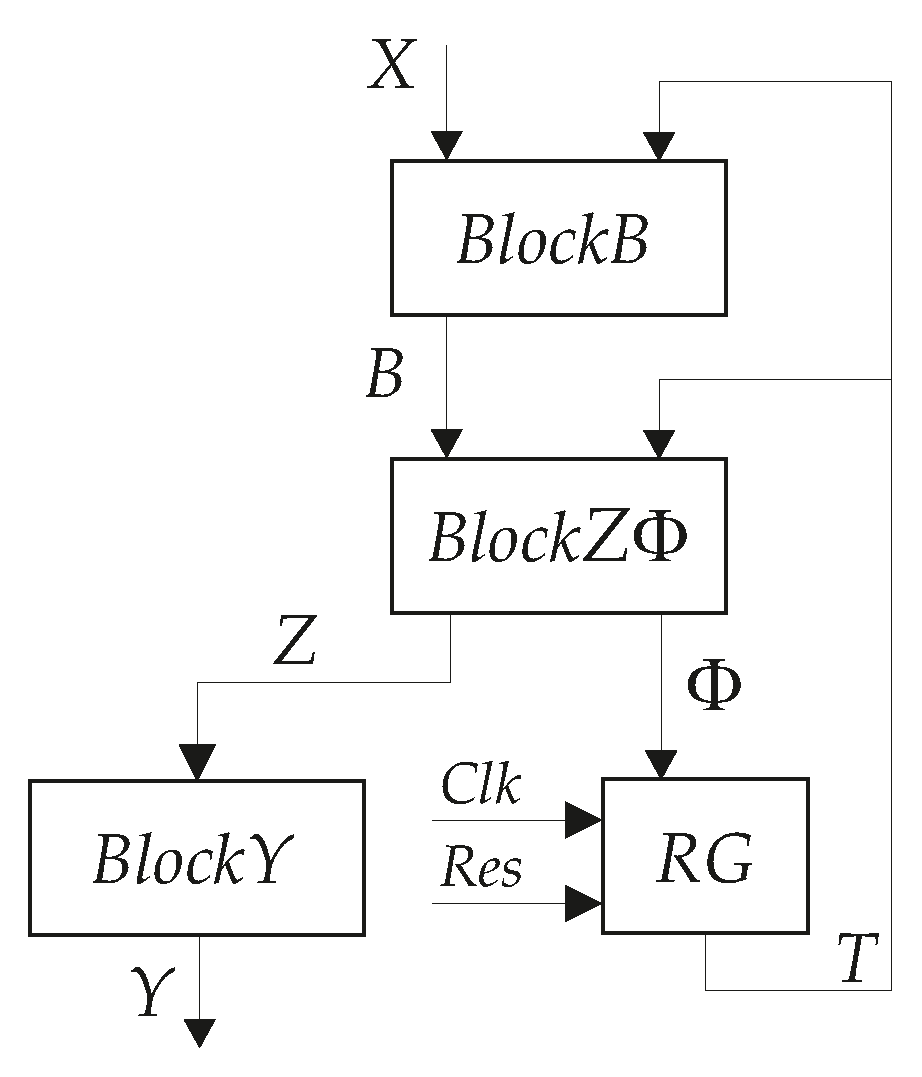
To do it, we should use different sets of variables to encode COs $Y\left(t\right)$ and $Y(t+1)$. For example, we use the elements of the set $Z=\{z_1,\dots ,z_{RQ}\}$ to encode a CO $Y(t+1)$ and the elements of a set $V=\{v_1,\dots ,v_{RQ}\}$ to encode a CO $Y\left(t\right)$. Obviously, this actually doubles the number of variables encoding the collections of outputs compared to (6). To avoid doubling the resources used for the encoding, we propose using two interconnected registers for storing the codes of COs. This approach results in FSM $U_3$ (Figure 6).

Figure 6. Structural diagram of LUT-based Mealy FSM $U_3$.

In FSM $U_3$, a block $LZ$ implements SBF (7). There is a distributed register $RZ$ inside of the block $LZ$. The register keeps the codes of COs $Y(t+1)$. This explains the presence of pulses Clk and Res entering $LZ$. The variables $z_r\in Z$ are inputs of both a block $LY$ and a register $RV$. The block $LY$ implements SBF (8). The register $RV$ de facto transforms the variables $z_r\in Z$ into the variables $v_r\in V$ representing the codes of COs $Y\left(t\right)$. As follows from Figure 6, the same pulses Clk and Res are used by both registers. A block $LT$ generates the state variables $T_r\in T$ represented by an SBF

$$T=T(Z,V).$$

(12)

There are the following product terms in SOPs of the SBF (12):

$$E_h=Z_h\wedge V_h(h\in \{1,\dots ,H_{ZV}\}).$$

(13)

In (13), the symbols $Z_h$ and $V_h$ stand for conjunctions of the variables $z_r\in Z$ and $v_r\in V$, respectively. As we show a bit later, the following condition can take place: $H\ne H_{ZV}$.

In this paper, we propose a synthesis method for $U_3$-based Mealy FSMs. We assume that the FSM to be synthesized is represented by its STG. The proposed method includes the following steps:

• Constructing the STT corresponding to an initial STG.
• Executing the state assignment using maximum binary codes $K\left(a_m\right)$.
• Encoding of collections of outputs $Y_q\subseteq Y$ by binary codes $K\left(Y_q\right)$.
• Finding the SBF $Y=Y\left(Z\right)$.
• Creating the modified DST of FSM $U_1$.
• Creating a table of pairs $P_g=<Y_i,Y_j>$ corresponding to pairs $<a_m,X_h>$.
• Creating a table representing the block $LZ$ and SBF $Z=Z(T,X)$.
• Creating a table representing the block $LT$ and SBF $T=T(Z,V)$.
• Implementing the LUT-based circuit of Mealy FSM $U_3$ using internal resources of a particular FPGA chip.

Let us analyze the complexity of the proposed method. Because each FSM transition should be transformed into a pair of COs, the time of synthesis depends on the number of FSM transitions. The synthesis algorithm does not include iterations. The pairs of COs are formed strictly sequentially: at each moment of time, the next in line transition is transformed into a pair of COs. In this regard, the algorithm has a linear character.

5. Example of Synthesis

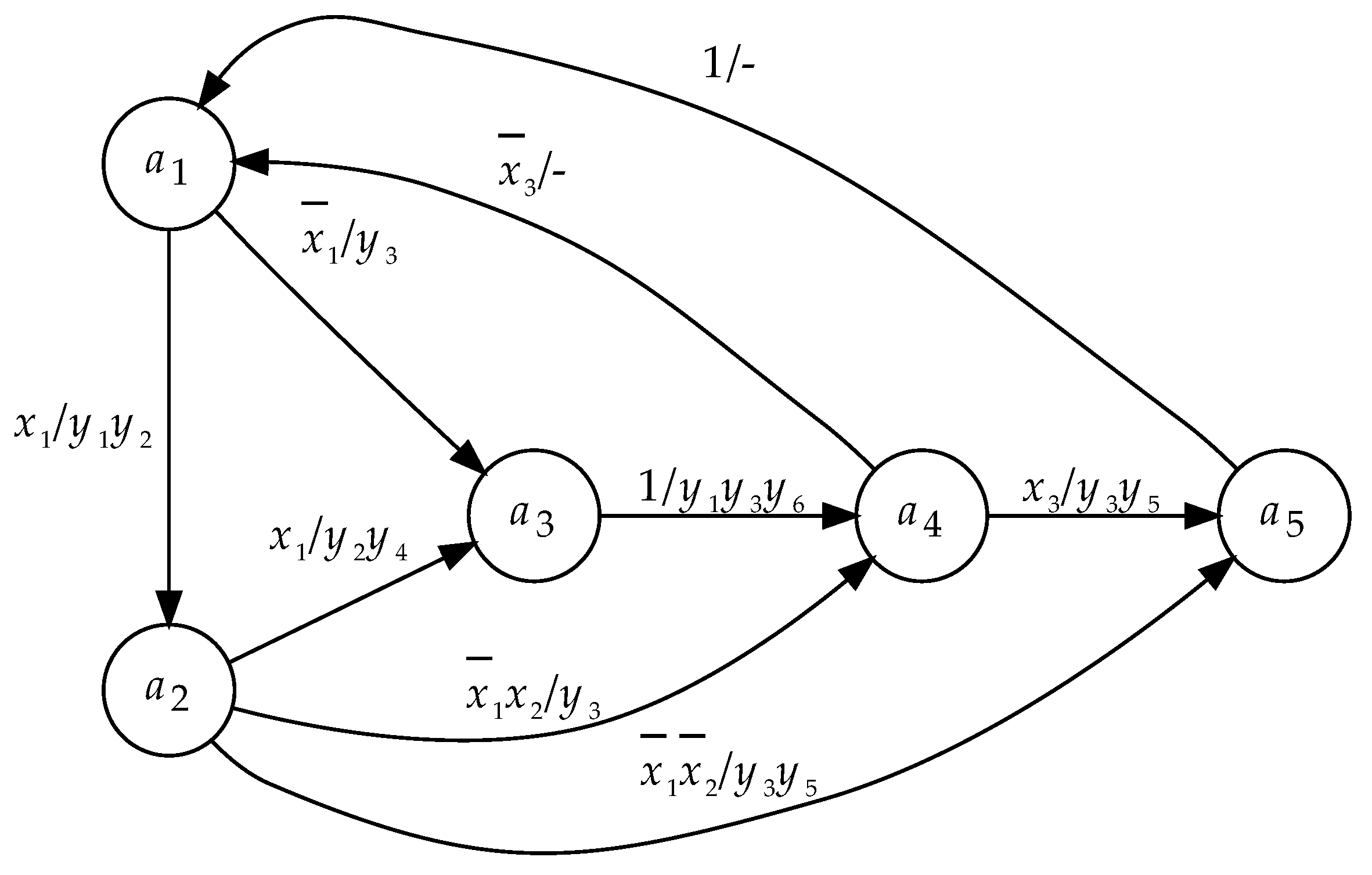
We use the symbol $U_i\left(S_a\right)$ to show that the model $U_i(i\in \{1,2,3\})$ of Mealy FSM is used to implement the circuit of an FSM $S_a$. Let us consider an example of the synthesis of Mealy FSM $U_3\left(S_1\right)$ shown in Figure 7. We use 4-LUTs to implement the circuit.

Figure 7. STG of Mealy FSM $S_1$.

Using an STG, we can find the sets of states, inputs and outputs, as well as the number of interstate transitions. Using Figure 7, we can find the sets $A=\{a_1,\dots ,a_5\}$, $X=\{x_1,x_2,x_3\}$ and $Y=\{y_1,\dots ,y_6\}$. This gives the following values: $M=3$, $L=3$, and $N=6$. The analysis of Figure 7 shows that there are $H=9$ transitions between the states of FSM $S_1$. Naturally, the state $a_1\in A$ is the initial state.

Step 1. The transformation of an STG into an equivalent STT is executed in the trivial way [16]. As follows from Figure 2, each arc of the STG is transformed in a row of the corresponding STT. In our case, Table 2 is an STT of Mealy FSM $S_1$ corresponding to the STG shown in Figure 7.

Table 2. State transition table of Mealy FSM $S_1$.

${\mathit{a}}_{\mathit{m}}$	${\mathit{a}}_{\mathit{T}}$	${\mathit{X}}_{\mathit{h}}$	${\mathit{Y}}_{\mathit{h}}$		h
$a_1$	$a_2$	$x_1$	$y_1{y}_2$	$Y_1$	1
	$a_3$	$\overline{x_1}$	$y_3$	$Y_2$	2
$a_2$	$a_3$	$x_1$	$y_2{y}_4$	$Y_3$	3
	$a_4$	$\overline{x_1}{x}_2$	$y_3$	$Y_2$	4
	$a_5$	$\overline{x_1}\overline{x_2}$	$y_3{y}_5$	$Y_4$	5
$a_3$	$a_4$	1	$y_1{y}_3{y}_6$	$Y_5$	6
$a_4$	$a_5$	$x_3$	$y_3{y}_5$	$Y_4$	7
	$a_1$	$\overline{x_3}$	–	$Y_0$	8
$a_5$	$a_1$	1	–	$Y_0$	9

In the column $Y_h$ of Table 2, we show the collections of outputs $Y_q\subseteq Y$. As a rule, such information is not given in the classical STT [5].

Step 2. For FSM $S_1$, there is $M=5$. Using (1) gives $R=3$. This determines the set of state variables $T=\{T_1,T_2,T_3\}$. It is possible to encode the states in a way optimizing the system (7). For example, this can be done using the algorithm JEDI [44]. In our simple example, we use the trivial way of state assignment [5] with the following state codes: $K\left(a_1\right)=000$, $K\left(a_2\right)=001$,…, $K\left(a_5\right)=100$.

Step 3. Using Table 2, we can find the following collections of outputs: $Y_0=Ø$, $Y_1=\{y_1,y_2\}$, $Y_2=\left\{y_3\right\}$, $Y_3=\{y_2,y_4\}$, $Y_4=\{y_3,y_5\}$, and $Y_5=\{y_1,y_3,y_6\}$. So, in our example, there is $Q=6$.

As shown in [13], it is necessary to encode the collections in a way that minimizes the number of literals in functions from (8). If the condition

$$R_Q>I$$

(14)

holds, then such an approach could minimize the LUT count for the block $LY$ [13,15,37].

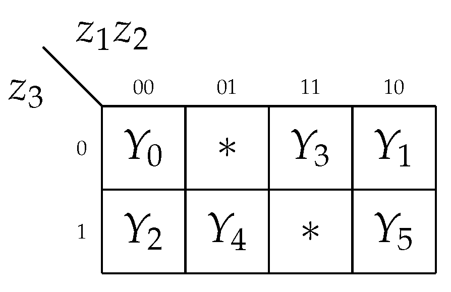
To encode the COs, we use the approach proposed in [55]. The outcome of encoding is shown in Figure 8.

Figure 8. The outcome of encoding of COs for FSM $S_1$.

Step 4. Using the distribution of FSM outputs by COs and codes (Figure 8), we obtain the following SBF:

$$\begin{array}{c}{y}_1=Y_1\vee Y_5=z_1\overline{z_2};\hfill \\ y_2=Y_1\vee Y_3=z_1\overline{z_3};\hfill \\ y_3=Y_2\vee Y_4\vee Y_5=z_3;\hfill \\ y_4=Y_3=z_1{z}_2;\hfill \\ y_5=Y_4=z_2{z}_3;\hfill \\ y_6=Y_5=z_1{z}_3;\hfill \end{array}$$

(15)

The analysis of (15) shows that there are 11 literals in this system. So, there are 11 interconnections between the blocks $LZ$ and $LY$. As shown in [13], in the common case, there are $N{R}_Q=21$ interconnections between these blocks. Therefore, using the approach [55] allows reducing the number of interconnections by 1.91 times.

Step 5. The columns of a DST are shown in Figure 2c. We have modified the traditional DST. The column $Y_h$ is replaced by a column $Z_h$ (Table 3).

Table 3. Modified DST of Mealy FSM $U_1\left(S_1\right)$.

${\mathit{a}}_{\mathit{m}}$	$\mathit{K}\left({\mathit{a}}_{\mathit{m}}\right)$	${\mathit{a}}_{\mathit{T}}$	$\mathit{K}\left({\mathit{a}}_{\mathit{T}}\right)$	${\mathit{X}}_{\mathit{h}}$	${\Phi }_{\mathit{h}}$	${\mathit{Z}}_{\mathit{h}}$	h
$a_1$	000	$a_2$	001	$x_1$	$D_3$	$z_1$	1
		$a_3$	010	$\overline{x_1}$	$D_2$	$z_3$	2
$a_2$	001	$a_3$	010	$x_1$	$D_2$	$z_1{z}_2$	3
		$a_4$	011	$\overline{x_1}{x}_2$	$D_2{D}_3$	$z_3$	4
		$a_5$	100	$\overline{x_1}\overline{x_2}$	$D_1$	$z_2{z}_3$	5
$a_3$	010	$a_4$	011	1	$D_2{D}_3$	$z_1{z}_3$	6
$a_4$	011	$a_5$	100	$x_3$	$D_1$	$z_2{z}_3$	7
		$a_1$	000	$\overline{x_3}$	–	–	8
$a_5$	100	$a_1$	000	1	–	–	9

Step 6. The first five steps of this example are performed using known techniques [13,15]. Starting from the sixth step, the features of our method appear. Since we propose to represent the terms of IMFs in the form of conjunctions corresponding to the codes of COs at adjacent operation cycles, it is necessary to find these pairs of COs. For these purposes, a table of pairs should be built.

A table of pairs $P_g=<Y_i,Y_j>$ shows a correspondence between these pairs and the pairs $<a_m,X_h>$. There are six columns in this table: $a_m$ (a current state); $a_T$ (a transition state); $Y_m$ (a CO produced during the transition into the state $a_m$); $Y_T$ (a CO produced during the interstate transition $<a_m,a_T>$); $P_g$ (a pair $<Y_m,Y_T>$); and g (the number of a table row, $g\in \{1,\dots ,G\}$). The following condition holds:

$$G\ge H.$$

(16)

For example, in the discussed case, there is $G=12$ (Table 4).

Table 4. Table of pairs $P_g$ for Mealy FSM $U_3\left(S_1\right)$.

${\mathit{a}}_{\mathit{m}}$	${\mathit{a}}_{\mathit{T}}$	${\mathit{Y}}_{\mathit{m}}$	${\mathit{Y}}_{\mathit{T}}$	${\mathit{P}}_{\mathit{g}}$	g
$a_1$	$a_2$	$Y_0$	$Y_1$	$P_1$	1
$a_1$	$a_3$	$Y_0$	$Y_2$	$P_2$	2
$a_2$	$a_3$	$Y_1$	$Y_3$	$P_3$	3
$a_2$	$a_4$	$Y_1$	$Y_2$	$P_4$	4
$a_2$	$a_5$	$Y_1$	$Y_4$	$P_5$	5
$a_3$	$a_4$	$Y_2$	$Y_5$	$P_6$	6
$a_3$	$a_4$	$Y_3$	$Y_5$	$P_7$	7
$a_4$	$a_5$	$Y_2$	$Y_4$	$P_8$	8
$a_4$	$a_1$	$Y_2$	$Y_0$	$P_9$	9
$a_4$	$a_5$	$Y_5$	$Y_4$	$P_{10}$	10
$a_4$	$a_1$	$Y_5$	$Y_0$	$P_{11}$	11
$a_5$	$a_1$	$Y_4$	$Y_0$	$P_{12}$	12

Let us explain why the relation (16) takes place. For example, there is a single transition $<a_3,a_4>$ in Table 2. This transition is accompanied by CO $Y_5$. At the same time, there are two rows in Table 4 representing this transition. This is explained by the fact that two different COs are produced during the transitions into $a_3\in A$. As follows from either the STG (Figure 7) or the STT (Table 2), the transition $<a_1,a_3>$ is accompanied by the generating CO $Y_2$ (the row 2 of Table 2), and the transition $<a_2,a_3>$ is accompanied by the generating CO $Y_3$ (the row 3 of Table 2). Due to it, the transition $<a_3,a_4>$ is represented by the pairs $P_6=<Y_2,Y_5>$ and $P_7=<Y_3,Y_5>$.

The similar analysis allows filling all rows of Table 4. Each transition from states $a_1,a_2,a_5\in A$ is represented by a single pair. However, two transitions from $a_4\in A$ are represented by four pairs $P_8-P_{11}$ (Table 4).

Step 7. The table of block $LZ$ (Table 5) is created using the modified DST (Table 3). This table includes only a part of the DST columns: $a_m,K\left(a_m\right),X_h;Z_h$ and h.

Table 5. Table of block $LZ$ of Mealy FSM $U_3\left(S_1\right)$.

${\mathit{a}}_{\mathit{m}}$	$\mathit{K}\left({\mathit{a}}_{\mathit{m}}\right)$	${\mathit{X}}_{\mathit{h}}$	${\mathit{Z}}_{\mathit{h}}$	h
$a_1$	000	$x_1$	$z_1$	1
		$\overline{x_1}$	$z_3$	2
$a_2$	001	$x_1$	$z_1{z}_2$	3
		$\overline{x_1}{x}_2$	$z_3$	4
		$\overline{x_1}\overline{x_2}$	$z_2{z}_3$	5
$a_3$	010	1	$z_1{z}_3$	6
$a_4$	011	$x_3$	$z_2{z}_3$	7
		$\overline{x_3}$	–	8
$a_5$	100	1	–	9

Obviously, SOPs of SBF (7) include the product terms $F_h=A_m{X}_h(h\in \{1,\dots ,H\})$. Using Table 5 gives the following minimized SOPs:

$$\begin{array}{c}{z}_1=(F_1\vee F_3)\vee F_6=\overline{T_1}\overline{T_2}{x}_1\vee \overline{T_1}{T}_2\overline{T_3};\hfill \\ z_2=F_3\vee F_5\vee F_7;\hfill \\ z_3=(F_2\vee F_4\vee F_5)\vee F_6\vee F_7=\overline{T_1}\overline{T_2}\overline{x_1}\vee T_2\overline{T_3}\vee T_2{T}_3{x}_3.\hfill \end{array}$$

(17)

Step 8. This step is presented only in our proposed method. As follows from (12), the state variables $T_r\in T$ depend on variables encoding COs. So, it is necessary to construct a table reflecting this dependence. To do it, each transition from the initial state transition table (Table 2) must be represented as a transition between the COs from the adjacent cycles of operation times. This dependence is shown in the table of $LT$.

The table of $LT$ includes seven columns. They are the following: $Y_m,$$K\left(Y_m\right),Y_T,K\left(Y_T\right)$, $a_T$$,T_g,$ and g. This table is constructed using the columns Y${}_m,Y_T,a_T$ of the table of pairs (Table 4), the codes of COs (Figure 8) and state codes $K\left(a_T\right)$. In the discussed case, there are $G=12$ rows in this table (Table 6).

Table 6. Table of block $LT$ of Mealy FSM $U_3\left(S_1\right)$.

${\mathit{Y}}_{\mathit{m}}$	$\mathit{K}\left({\mathit{Y}}_{\mathit{m}}\right)$	${\mathit{Y}}_{\mathit{T}}$	$\mathit{K}\left({\mathit{Y}}_{\mathit{T}}\right)$	${\mathit{a}}_{\mathit{T}}$	${\mathit{T}}_{\mathit{g}}$	g
$Y_0$	000	$Y_1$	100	$a_2$	$T_3$	1
$Y_0$	000	$Y_2$	001	$a_3$	$T_2$	2
$Y_1$	100	$Y_3$	110	$a_3$	$T_2$	3
$Y_1$	100	$Y_2$	001	$a_4$	$T_2{T}_3$	4
$Y_1$	100	$Y_4$	011	$a_5$	$T_1$	5
$Y_2$	001	$Y_5$	101	$a_4$	$T_2{T}_3$	6
$Y_3$	110	$Y_5$	101	$a_4$	$T_2{T}_3$	7
$Y_2$	001	$Y_4$	011	$a_5$	$T_1$	8
$Y_2$	001	$Y_0$	000	$a_1$	–	9
$Y_5$	101	$Y_4$	011	$a_5$	$T_1$	10
$Y_5$	101	$Y_0$	000	$a_1$	–	11
$Y_4$	011	$Y_0$	000	$a_1$	–	12

For example, the following relations take places for the first row of Table 4: $Y_m=Y_0$, $Y_T=Y_1$ and $a_T=a_2$. As follows from Figure 8, there are the codes $K\left(Y_0\right)=000$ and $K\left(Y_1\right)=100$. As follows, for example, from Table 5, there is the state code $K\left(a_2\right)=001$. So, the column $T_g$ of Table 6 contains the symbol $T_3$ for the row g = 1. All other rows are filled in the same manner.

Using the table of $LT$, the SBF (12) is derived. The SOPs of corresponding functions include the terms (13). In the discussed case, this is the following SBF:

$$\begin{array}{c}{T}_1=P_5\vee P_8\vee P_{10}=v_1\overline{v_2}\overline{v_3}\overline{z_1}{z}_2\vee \overline{v_1}\overline{v_2}{v}_3\overline{z_1}{z}_2\vee v_1{v}_3\overline{z_1}{z}_2;\hfill \\ T_2=P_2\vee P_3\vee P_4\vee P_6\vee P_7;\hfill \\ T_3=P_4\vee P_6\vee P_7.\hfill \end{array}$$

(18)

Step 9. To obtain the LUT-based circuit of Mealy FSM $U_3\left(S_1\right)$, the step of technology mapping should be executed [31]. This can be done only with the help of some industrial CAD tools. In the case of Virtex-7-based circuits, the industrial package Vivado [47] should be used. This CAD tool executes the process of technology mapping. As a result, we can extract the real characteristics of an FSM circuit (such as the LUT count, number of slices, number of flip-flops, maximum operating frequency, and power consumption) from the Vivado reports.

This CAD tool can be used starting from the FPGAs of the Virtex-7 family. So, it is impossible to use Vivado for implementing the circuit of FSM $U_3\left(S_1\right)$ using LUTs with four inputs. In the next section, there are shown the results of experiments conducted with the help of the industrial CAD package Vivado and the library of standard benchmark FSMs [56].

6. Experimental Results

In this section, there are shown the results of experiments which were conducted to compare the characteristics of $U_3$-based Mealy FSMs with the characteristics of FSM circuits based on some other models. The benchmark FSMs from the library [56] are used for these experiments. This library includes 48 benchmarks represented in the format KISS2 taken from the practice of logic design. Although the library dates back to the 1990s of the twentieth century, it has been used by various authors for 30 years to compare the new and existing methods of implementing FSM circuits. Let us indicate only some examples of articles and monographs, where the library [56] is used in experimental research. Such works include, for example, articles [31,35,52,57,58,59] and monographs [6,39]. The basic characteristics of benchmarks are shown in Table 7.

Table 7. Basic characteristics of benchmarks from library [56].

Benchmark	L	N	$\mathit{R}+\mathit{L}$	$\mathit{M}/\mathit{R}$	H	Group
bbara	4	2	8	12/4	60	1
bbsse	7	7	12	26/5	56	1
bbtas	2	2	6	9/4	24	0
beecount	3	4	7	10/4	28	1
cse	7	7	12	32/5	91	1
dk14	3	5	8	26/5	56	1
dk15	3	5	8	17/5	32	1
dk16	2	3	9	75/7	108	1
dk17	2	3	6	16/4	32	0
dk27	1	2	5	10/4	14	0
dk512	1	3	6	24/5	15	0
donfile	2	1	7	24/5	96	1
ex1	9	19	16	80/7	138	2
ex2	2	2	7	25/5	72	1
ex3	2	2	6	14/4	36	0
ex4	6	9	11	18/5	21	1
ex5	2	2	6	16/4	32	0
ex6	5	8	9	14/4	34	1
ex7	2	2	12	17/5	36	1
keyb	7	7	12	22/5	170	1
kirkman	12	6	18	48/6	370	2
lion	2	1	5	5/3	11	0
lion9	2	1	6	11/4	25	0
mark1	5	16	10	22/5	22	1
mc	3	5	6	8/3	10	0
modulo12	1	1	5	12/4	24	0
opus	5	6	10	18/5	22	1
planet	7	19	14	86/7	115	2
planet1	7	19	14	86/7	115	2
pma	8	8	14	49/6	73	2
s1	8	7	14	54/6	106	2
s1488	8	19	15	112/7	251	2
s1494	8	19	15	118/7	250	2
s1a	8	6	15	86/7	107	2
s208	11	2	17	37/6	153	2
s27	4	1	8	11/4	34	1
s386	7	7	12	23/5	64	1
s420	19	2	27	137/8	137	4
s510	19	7	27	172/8	77	4
s8	4	1	8	15/4	20	1
s820	18	19	25	78/7	232	4
s832	18	19	25	76/7	245	4
sand	11	9	18	88/7	184	3
shiftreg	1	1	5	16/4	16	0
sse	7	7	12	26/5	56	1
styr	9	10	16	67/7	166	2
tma	7	9	13	63/6	44	2

To conduct the research, we use a personal computer with the following characteristics: CPU, Intel Core i7 6700 K 4.2@4.4 GHz and memory, 16 GB RAM 2400MHz CL15. As a platform for FSM circuits implementation, the Virtex-7 VC709 Evaluation Platform (xc7vx690tffg1761-2) [60] is used. As a CAD tool, we use the package Vivado v2019.1 (64-bit) of Xilinx [47]. The circuits are implemented using CLBs from the slices SLICEL. They include LUTs having six inputs. To create the tables with research results, the reports of Vivado are used. To link the initial KISS2-based files with Vivado, we create VHDL-based descriptions of these models. To do it, the CAD tool K2F [40] is used.

Using the Vivado reports, we compare some parameters of produced FSM circuits. These parameters are (1) the required chip area occupied by an FSM circuit (the LUT count represents this characteristic); (2) the maximum operating frequency achievable for a particular FSM; (3) the required number of flip-flops; (4) the power consumption; (5) the area-time products; and (6) the power–time products. In our experiments, we use the following FSM models: (1) auto of Vivado (it is based on the maximum binary state codes); (2) one-hot of Vivado (in this case, $R=M$); (3) JEDI; (4) $U_2$-based FSMs [15]; and (5) $U_3$-based FSMs proposed in this article.

As it is in our previous research [15], the benchmark FSMs are divided by five groups. The groups are determined by the value of a parameter $D(R,L,I)$. This parameter is calculated as

$$D(R,L,I)=L+R-I.$$

(19)

Using (19), we create the following groups. The relation $D(R,L,I)\le 0$ determines the group of trivial FSMs (the group G0). The relation $0<D(R,L,I)\le 6$ determines the group of simple FSMs (G1). The relation $6<D(R,L,I)\le 12$ determines the group of average FSMs (G2). The relation $12<D(R,L,I)\le 18$ determines the group of big FSMs (G3). The relation $D(R,L,I)>18$ determines the group of very big FSMs (G4). As research [15] shows, the larger the group number, the greater the gain from the use of methods of structural decomposition.

The results of the experiments are shown in Table 8, Table 9, Table 10, Table 11, Table 12, Table 13, Table 14, Table 15, Table 16, Table 17, Table 18, Table 19 and Table 20. We have organized these tables in the following way. In the table columns, we show the names of the methods used. The table rows are marked by the names of benchmarks. At the intersection of a column with a method and a row with a benchmark, we show the result of a specific experiment obtained from the Vivado report. Inside each table, the benchmarks are listed in alphabetical order and sorted by ascending group number. The rows “Total” contain the results of summation of values for each column. The row “Percentage” includes the percentage of summarized characteristics of FSM circuits produced by other methods, respectively, to $U_3$-based FSMs. We use the model of Mealy FSM $U_1$ for methods auto, one-hot, and JEDI.

These tables include the following information: (1) the LUT counts for all benchmarks (Table 8); (2) the LUT counts for benchmarks of the group G0 (Table 9); (3) the LUT counts for benchmarks of the group G1 (Table 10); (4) the LUT counts for benchmarks of groups G2, G3 and G4 (Table 11); (5) the maximum operating frequency for all benchmarks (Table 12); (6) the maximum operating frequency for benchmarks of the group G0 (Table 13); (7) the maximum operating frequency for benchmarks of the group G1 (Table 14); and (8) the maximum operating frequency for benchmarks of the groups G2–G4 (Table 15).

To fill in the tables with the research results, we use data from our previous articles. Basically, all numbers are taken from papers [13,61]. However, information about the number of flip-flops is mentioned only in paper [14]. Therefore, we used Ref. [14] to fill in Table 16. The necessary information regarding the proposed method is taken from the Vivado reports.

The following conclusions can be made from the analysis of Table 8, Table 9, Table 10, Table 11, Table 12, Table 13, Table 14 and Table 15.

Table 8. Experimental results (LUT counts for all benchmarks).

Benchmark	Auto [13]	One-Hot [13]	JEDI [14]	${\mathit{U}}_2$ [61]	Our Approach	Group
bbtas	5	5	5	8	8	0
dk17	5	12	5	8	8	0
dk27	3	5	4	7	7	0
dk512	10	10	9	12	13	0
ex3	9	9	9	11	11	0
ex5	9	9	9	10	10	0
lion	2	5	2	6	6	0
lion9	6	11	5	8	8	0
mc	4	7	4	6	6	0
modulo12	7	7	7	9	9	0
shiftreg	2	6	2	4	4	0
bbara	17	17	10	10	11	1
bbsse	33	37	24	26	24	1
beecount	19	19	14	14	13	1
cse	40	66	36	33	32	1
dk14	16	27	10	12	11	1
dk15	15	16	12	6	7	1
dk16	15	34	12	11	10	1
donfile	31	31	24	21	20	1
ex2	9	9	8	8	9	1
ex4	15	13	12	11	10	1
ex6	24	36	22	21	20	1
ex7	4	5	4	6	7	1
keyb	43	61	40	37	38	1
mark1	23	23	20	19	18	1
opus	28	28	22	21	20	1
s27	6	18	6	6	7	1
s386	26	39	22	25	22	1
s8	9	9	9	9	10	1
sse	33	37	30	26	25	1
ex1	70	74	53	40	34	2
kirkman	42	58	39	33	29	2
planet	131	131	88	78	71	2
planet1	131	131	88	78	71	2
pma	94	94	86	72	68	2
s1	65	99	61	54	50	2
s1488	124	131	108	89	86	2
s1494	126	132	110	90	80	2
s1a	49	81	43	38	34	2
s208	12	31	10	9	11	2
styr	93	120	81	70	62	2
tma	45	39	39	30	29	2
sand	132	132	114	99	82	3
s420	10	31	9	8	9	4
s510	48	48	32	22	20	4
s820	88	82	68	52	48	4
s832	80	79	62	50	46	4
Total	1808	2104	1489	1323	1234
Percentage,%	146.52	170.50	120.66	107.21	100.00

Table 8. Experimental results (LUT counts for all benchmarks).

Benchmark	Auto [13]	One-Hot [13]	JEDI [14]	${\mathit{U}}_2$ [61]	Our Approach	Group
bbtas	5	5	5	8	8	0
dk17	5	12	5	8	8	0
dk27	3	5	4	7	7	0
dk512	10	10	9	12	13	0
ex3	9	9	9	11	11	0
ex5	9	9	9	10	10	0
lion	2	5	2	6	6	0
lion9	6	11	5	8	8	0
mc	4	7	4	6	6	0
modulo12	7	7	7	9	9	0
shiftreg	2	6	2	4	4	0
bbara	17	17	10	10	11	1
bbsse	33	37	24	26	24	1
beecount	19	19	14	14	13	1
cse	40	66	36	33	32	1
dk14	16	27	10	12	11	1
dk15	15	16	12	6	7	1
dk16	15	34	12	11	10	1
donfile	31	31	24	21	20	1
ex2	9	9	8	8	9	1
ex4	15	13	12	11	10	1
ex6	24	36	22	21	20	1
ex7	4	5	4	6	7	1
keyb	43	61	40	37	38	1
mark1	23	23	20	19	18	1
opus	28	28	22	21	20	1
s27	6	18	6	6	7	1
s386	26	39	22	25	22	1
s8	9	9	9	9	10	1
sse	33	37	30	26	25	1
ex1	70	74	53	40	34	2
kirkman	42	58	39	33	29	2
planet	131	131	88	78	71	2
planet1	131	131	88	78	71	2
pma	94	94	86	72	68	2
s1	65	99	61	54	50	2
s1488	124	131	108	89	86	2
s1494	126	132	110	90	80	2
s1a	49	81	43	38	34	2
s208	12	31	10	9	11	2
styr	93	120	81	70	62	2
tma	45	39	39	30	29	2
sand	132	132	114	99	82	3
s420	10	31	9	8	9	4
s510	48	48	32	22	20	4
s820	88	82	68	52	48	4
s832	80	79	62	50	46	4
Total	1808	2104	1489	1323	1234
Percentage,%	146.52	170.50	120.66	107.21	100.00

Table 9. Experimental results (LUT counts for benchmarks of G0).

Benchmark	Auto [13]	One-Hot [13]	JEDI [14]	${\mathit{U}}_2$ [61]	Our Approach
bbtas	5	5	5	8	8
dk17	5	12	5	8	8
dk27	3	5	4	7	7
dk512	10	10	9	12	13
ex3	9	9	9	11	11
ex5	9	9	9	10	10
lion	2	5	2	6	6
lion9	6	11	5	8	8
mc	4	7	4	6	6
modulo12	7	7	7	9	9
shiftreg	2	6	2	4	4
Total	62	86	61	89	90
Percentage,%	68.89	95.56	67.78	98.89	100.00

Table 9. Experimental results (LUT counts for benchmarks of G0).

Benchmark	Auto [13]	One-Hot [13]	JEDI [14]	${\mathit{U}}_2$ [61]	Our Approach
bbtas	5	5	5	8	8
dk17	5	12	5	8	8
dk27	3	5	4	7	7
dk512	10	10	9	12	13
ex3	9	9	9	11	11
ex5	9	9	9	10	10
lion	2	5	2	6	6
lion9	6	11	5	8	8
mc	4	7	4	6	6
modulo12	7	7	7	9	9
shiftreg	2	6	2	4	4
Total	62	86	61	89	90
Percentage,%	68.89	95.56	67.78	98.89	100.00

Table 10. Experimental results (LUT counts for benchmarks of G1).

Benchmark	Auto [13]	One-Hot [13]	JEDI [14]	${\mathit{U}}_2$ [61]	Our Approach
bbara	17	17	10	10	11
bbsse	33	37	24	26	24
beecount	19	19	14	14	13
cse	40	66	36	33	32
dk14	16	27	10	12	11
dk15	15	16	12	6	7
dk16	15	34	12	11	10
donfile	31	31	24	21	20
ex2	9	9	8	8	9
ex4	15	13	12	11	10
ex6	24	36	22	21	20
ex7	4	5	4	6	7
keyb	43	61	40	37	38
mark1	23	23	20	19	18
opus	28	28	22	21	20
s27	6	18	6	6	7
s386	26	39	22	25	22
s8	9	9	9	9	10
sse	33	37	30	26	25
Total	406	525	337	322	314
Percentage,%	129.30	167.20	107.32	102.55	100.00

Table 10. Experimental results (LUT counts for benchmarks of G1).

Benchmark	Auto [13]	One-Hot [13]	JEDI [14]	${\mathit{U}}_2$ [61]	Our Approach
bbara	17	17	10	10	11
bbsse	33	37	24	26	24
beecount	19	19	14	14	13
cse	40	66	36	33	32
dk14	16	27	10	12	11
dk15	15	16	12	6	7
dk16	15	34	12	11	10
donfile	31	31	24	21	20
ex2	9	9	8	8	9
ex4	15	13	12	11	10
ex6	24	36	22	21	20
ex7	4	5	4	6	7
keyb	43	61	40	37	38
mark1	23	23	20	19	18
opus	28	28	22	21	20
s27	6	18	6	6	7
s386	26	39	22	25	22
s8	9	9	9	9	10
sse	33	37	30	26	25
Total	406	525	337	322	314
Percentage,%	129.30	167.20	107.32	102.55	100.00

Table 11. Experimental results (LUT counts for benchmarks of G2–G4).

Benchmark	Auto [13]	One-Hot [13]	JEDI [14]	${\mathit{U}}_2$ [61]	Our Approach
ex1	70	74	53	40	34
kirkman	42	58	39	33	29
planet	131	131	88	78	71
planet1	131	131	88	78	71
pma	94	94	86	72	68
s1	65	99	61	54	50
s1488	124	131	108	89	86
s1494	126	132	110	90	80
s1a	49	81	43	38	34
s208	12	31	10	9	11
styr	93	120	81	70	62
tma	45	39	39	30	29
sand	132	132	114	99	82
s420	10	31	9	8	9
s510	48	48	32	22	20
s820	88	82	68	52	48
s832	80	79	62	50	46
Total	1340	1493	1091	912	830
Percentage,%	161.45	179.88	131.45	109.88	100.00

Table 11. Experimental results (LUT counts for benchmarks of G2–G4).

Benchmark	Auto [13]	One-Hot [13]	JEDI [14]	${\mathit{U}}_2$ [61]	Our Approach
ex1	70	74	53	40	34
kirkman	42	58	39	33	29
planet	131	131	88	78	71
planet1	131	131	88	78	71
pma	94	94	86	72	68
s1	65	99	61	54	50
s1488	124	131	108	89	86
s1494	126	132	110	90	80
s1a	49	81	43	38	34
s208	12	31	10	9	11
styr	93	120	81	70	62
tma	45	39	39	30	29
sand	132	132	114	99	82
s420	10	31	9	8	9
s510	48	48	32	22	20
s820	88	82	68	52	48
s832	80	79	62	50	46
Total	1340	1493	1091	912	830
Percentage,%	161.45	179.88	131.45	109.88	100.00

Table 12. Experimental results (the maximum operating frequency for all benchmarks).

Benchmark	Auto [13]	One-Hot [13]	JEDI [14]	${\mathit{U}}_2$ [14]	Our Approach	Group
bbtas	204.16	204.16	206.12	200.38	199.48	0
dk17	199.28	167	199.39	199.87	198.03	0
dk27	206.02	201.9	204.18	196.65	194.18	0
dk512	196.27	196.27	199.75	194.17	192.34	0
ex3	194.86	194.86	195.76	191.22	188.14	0
ex5	180.25	180.25	181.16	178.06	176.74	0
lion	202.43	204	202.35	200.18	199.12	0
lion9	205.3	185.22	206.38	199.12	197.07	0
mc	196.66	195.47	196.87	193.17	191.52	0
modulo12	207	207	207.13	201.12	200.23	0
shiftreg	262.67	263.57	276.26	256.69	253.24	0
bbara	193.39	193.39	212.21	202.23	201.12	1
bbsse	157.06	169.12	182.34	181.23	178.64	1
beecount	166.61	166.61	187.32	185.14	183.72	1
cse	146.43	163.64	178.12	175.18	172.42	1
dk14	191.64	172.65	193.85	190.18	188.86	1
dk15	192.53	185.36	194.87	192.23	191.48	1
dk16	169.72	174.79	197.13	194.34	192.83	1
donfile	184.03	184	203.65	200.92	198.47	1
ex2	198.57	198.57	200.14	198.32	197.26	1
ex4	180.96	177.71	192.83	190.14	188.32	1
ex6	169.57	163.8	176.59	171.27	170.18	1
ex7	200.04	200.84	200.6	198.14	197.38	1
keyb	156.45	143.47	168.43	162.01	161.25	1
mark1	162.39	162.39	176.18	170.18	168.04	1
opus	166.2	166.2	178.32	175.29	173.41	1
s27	198.73	191.5	199.13	196.13	194.17	1
s386	168.15	173.46	179.15	176.85	174.62	1
s8	180.02	178.95	181.23	178.23	176.22	1
sse	157.06	169.12	174.63	170.12	167.43	1
ex1	150.94	139.76	176.87	182.34	180.01	2
kirkman	141.38	154	156.68	167.15	165.62	2
planet	132.71	132.71	187.14	189.12	187.07	2
planet1	132.71	132.71	187.14	189.12	187.07	2
pma	146.18	146.18	169.83	178.19	176.26	2
s1	146.41	135.85	157.16	162.23	164.12	2
s1488	138.5	131.94	157.18	168.32	167.14	2
s1494	149.39	145.75	164.34	172.27	170.95	2
s1a	153.37	176.4	169.17	178.21	176.25	2
s208	174.34	176.46	178.76	181.72	180.29	2
styr	137.61	129.92	145.64	161.87	159.25	2
tma	163.88	147.8	164.14	176.72	175.06	2
sand	115.97	115.97	126.82	145.68	152.49	3
s420	173.88	176.46	177.25	187.23	190.56	4
s510	177.65	177.65	181.42	187.32	190.24	4
s820	152	153.16	176.58	181.96	183.12	4
s832	145.71	153.23	173.78	186.12	187.45	4
Total	8127.08	8061.22	8701.97	8536.27	8658.86
Percentage,%	93.86	93.10	100.50	98.58	100.00

Table 12. Experimental results (the maximum operating frequency for all benchmarks).

Benchmark	Auto [13]	One-Hot [13]	JEDI [14]	${\mathit{U}}_2$ [14]	Our Approach	Group
bbtas	204.16	204.16	206.12	200.38	199.48	0
dk17	199.28	167	199.39	199.87	198.03	0
dk27	206.02	201.9	204.18	196.65	194.18	0
dk512	196.27	196.27	199.75	194.17	192.34	0
ex3	194.86	194.86	195.76	191.22	188.14	0
ex5	180.25	180.25	181.16	178.06	176.74	0
lion	202.43	204	202.35	200.18	199.12	0
lion9	205.3	185.22	206.38	199.12	197.07	0
mc	196.66	195.47	196.87	193.17	191.52	0
modulo12	207	207	207.13	201.12	200.23	0
shiftreg	262.67	263.57	276.26	256.69	253.24	0
bbara	193.39	193.39	212.21	202.23	201.12	1
bbsse	157.06	169.12	182.34	181.23	178.64	1
beecount	166.61	166.61	187.32	185.14	183.72	1
cse	146.43	163.64	178.12	175.18	172.42	1
dk14	191.64	172.65	193.85	190.18	188.86	1
dk15	192.53	185.36	194.87	192.23	191.48	1
dk16	169.72	174.79	197.13	194.34	192.83	1
donfile	184.03	184	203.65	200.92	198.47	1
ex2	198.57	198.57	200.14	198.32	197.26	1
ex4	180.96	177.71	192.83	190.14	188.32	1
ex6	169.57	163.8	176.59	171.27	170.18	1
ex7	200.04	200.84	200.6	198.14	197.38	1
keyb	156.45	143.47	168.43	162.01	161.25	1
mark1	162.39	162.39	176.18	170.18	168.04	1
opus	166.2	166.2	178.32	175.29	173.41	1
s27	198.73	191.5	199.13	196.13	194.17	1
s386	168.15	173.46	179.15	176.85	174.62	1
s8	180.02	178.95	181.23	178.23	176.22	1
sse	157.06	169.12	174.63	170.12	167.43	1
ex1	150.94	139.76	176.87	182.34	180.01	2
kirkman	141.38	154	156.68	167.15	165.62	2
planet	132.71	132.71	187.14	189.12	187.07	2
planet1	132.71	132.71	187.14	189.12	187.07	2
pma	146.18	146.18	169.83	178.19	176.26	2
s1	146.41	135.85	157.16	162.23	164.12	2
s1488	138.5	131.94	157.18	168.32	167.14	2
s1494	149.39	145.75	164.34	172.27	170.95	2
s1a	153.37	176.4	169.17	178.21	176.25	2
s208	174.34	176.46	178.76	181.72	180.29	2
styr	137.61	129.92	145.64	161.87	159.25	2
tma	163.88	147.8	164.14	176.72	175.06	2
sand	115.97	115.97	126.82	145.68	152.49	3
s420	173.88	176.46	177.25	187.23	190.56	4
s510	177.65	177.65	181.42	187.32	190.24	4
s820	152	153.16	176.58	181.96	183.12	4
s832	145.71	153.23	173.78	186.12	187.45	4
Total	8127.08	8061.22	8701.97	8536.27	8658.86
Percentage,%	93.86	93.10	100.50	98.58	100.00

Table 13. Experimental results (the maximum operating frequency for G0).

Benchmark	Auto [13]	One-Hot [13]	JEDI [14]	${\mathit{U}}_2$ [14]	Our Approach
bbtas	204.16	204.16	206.12	200.38	199.48
dk17	199.28	167	199.39	199.87	198.03
dk27	206.02	201.9	204.18	196.65	194.18
dk512	196.27	196.27	199.75	194.17	192.34
ex3	194.86	194.86	195.76	191.22	188.14
ex5	180.25	180.25	181.16	178.06	176.74
lion	202.43	204	202.35	200.18	199.12
lion9	205.3	185.22	206.38	199.12	197.07
mc	196.66	195.47	196.87	193.17	191.52
modulo12	207	207	207.13	201.12	200.23
shiftreg	262.67	263.57	276.26	256.69	253.24
Total	2254.90	2199.70	2275.35	2032.57	2190.09
Percentage,%	102.96	100.44	103.89	92.81	100.00

Table 13. Experimental results (the maximum operating frequency for G0).

Benchmark	Auto [13]	One-Hot [13]	JEDI [14]	${\mathit{U}}_2$ [14]	Our Approach
bbtas	204.16	204.16	206.12	200.38	199.48
dk17	199.28	167	199.39	199.87	198.03
dk27	206.02	201.9	204.18	196.65	194.18
dk512	196.27	196.27	199.75	194.17	192.34
ex3	194.86	194.86	195.76	191.22	188.14
ex5	180.25	180.25	181.16	178.06	176.74
lion	202.43	204	202.35	200.18	199.12
lion9	205.3	185.22	206.38	199.12	197.07
mc	196.66	195.47	196.87	193.17	191.52
modulo12	207	207	207.13	201.12	200.23
shiftreg	262.67	263.57	276.26	256.69	253.24
Total	2254.90	2199.70	2275.35	2032.57	2190.09
Percentage,%	102.96	100.44	103.89	92.81	100.00

Table 14. Experimental results (the maximum operating frequency for G1).

Benchmark	Auto [13]	One-Hot [13]	JEDI [14]	${\mathit{U}}_2$ [14]	Our Approach
bbara	193.39	193.39	212.21	202.23	201.12
bbsse	157.06	169.12	182.34	181.23	178.64
beecount	166.61	166.61	187.32	185.14	183.72
cse	146.43	163.64	178.12	175.18	172.42
dk14	191.64	172.65	193.85	190.18	188.86
dk15	192.53	185.36	194.87	192.23	191.48
dk16	169.72	174.79	197.13	194.34	192.83
donfile	184.03	184	203.65	200.92	198.47
ex2	198.57	198.57	200.14	198.32	197.26
ex4	180.96	177.71	192.83	190.14	188.32
ex6	169.57	163.8	176.59	171.27	170.18
ex7	200.04	200.84	200.6	198.14	197.38
keyb	156.45	143.47	168.43	162.01	161.25
mark1	162.39	162.39	176.18	170.18	168.04
opus	166.2	166.2	178.32	175.29	173.41
s27	198.73	191.5	199.13	196.13	194.17
s386	168.15	173.46	179.15	176.85	174.62
s8	180.02	178.95	181.23	178.23	176.22
sse	157.06	169.12	174.63	170.12	167.43
Total	3339.55	3335.57	3576.72	3508.13	3475.82
Percentage,%	96.08	95.96	102.90	100.93	100.00

Table 14. Experimental results (the maximum operating frequency for G1).

Benchmark	Auto [13]	One-Hot [13]	JEDI [14]	${\mathit{U}}_2$ [14]	Our Approach
bbara	193.39	193.39	212.21	202.23	201.12
bbsse	157.06	169.12	182.34	181.23	178.64
beecount	166.61	166.61	187.32	185.14	183.72
cse	146.43	163.64	178.12	175.18	172.42
dk14	191.64	172.65	193.85	190.18	188.86
dk15	192.53	185.36	194.87	192.23	191.48
dk16	169.72	174.79	197.13	194.34	192.83
donfile	184.03	184	203.65	200.92	198.47
ex2	198.57	198.57	200.14	198.32	197.26
ex4	180.96	177.71	192.83	190.14	188.32
ex6	169.57	163.8	176.59	171.27	170.18
ex7	200.04	200.84	200.6	198.14	197.38
keyb	156.45	143.47	168.43	162.01	161.25
mark1	162.39	162.39	176.18	170.18	168.04
opus	166.2	166.2	178.32	175.29	173.41
s27	198.73	191.5	199.13	196.13	194.17
s386	168.15	173.46	179.15	176.85	174.62
s8	180.02	178.95	181.23	178.23	176.22
sse	157.06	169.12	174.63	170.12	167.43
Total	3339.55	3335.57	3576.72	3508.13	3475.82
Percentage,%	96.08	95.96	102.90	100.93	100.00

Table 15. Experimental results (the maximum operating frequency for G2–G4).

Benchmark	Auto [13]	One-Hot [13]	JEDI [14]	${\mathit{U}}_2$ [14]	Our Approach
ex1	150.94	139.76	176.87	182.34	180.01
kirkman	141.38	154	156.68	167.15	165.62
planet	132.71	132.71	187.14	189.12	187.07
planet1	132.71	132.71	187.14	189.12	187.07
pma	146.18	146.18	169.83	178.19	176.26
s1	146.41	135.85	157.16	162.23	164.12
s1488	138.5	131.94	157.18	168.32	167.14
s1494	149.39	145.75	164.34	172.27	170.95
s1a	153.37	176.4	169.17	178.21	176.25
s208	174.34	176.46	178.76	181.72	180.29
styr	137.61	129.92	145.64	161.87	159.25
tma	163.88	147.8	164.14	176.72	175.06
sand	115.97	115.97	126.82	145.68	152.49
s420	173.88	176.46	177.25	187.23	190.56
s510	177.65	177.65	181.42	187.32	190.24
s820	152	153.16	176.58	181.96	183.12
s832	145.71	153.23	173.78	186.12	187.45
Total	2532.63	2525.95	2849.90	2995.57	2992.95
Percentage,%	84.62	84.40	95.22	100.09	100.00

Table 15. Experimental results (the maximum operating frequency for G2–G4).

Benchmark	Auto [13]	One-Hot [13]	JEDI [14]	${\mathit{U}}_2$ [14]	Our Approach
ex1	150.94	139.76	176.87	182.34	180.01
kirkman	141.38	154	156.68	167.15	165.62
planet	132.71	132.71	187.14	189.12	187.07
planet1	132.71	132.71	187.14	189.12	187.07
pma	146.18	146.18	169.83	178.19	176.26
s1	146.41	135.85	157.16	162.23	164.12
s1488	138.5	131.94	157.18	168.32	167.14
s1494	149.39	145.75	164.34	172.27	170.95
s1a	153.37	176.4	169.17	178.21	176.25
s208	174.34	176.46	178.76	181.72	180.29
styr	137.61	129.92	145.64	161.87	159.25
tma	163.88	147.8	164.14	176.72	175.06
sand	115.97	115.97	126.82	145.68	152.49
s420	173.88	176.46	177.25	187.23	190.56
s510	177.65	177.65	181.42	187.32	190.24
s820	152	153.16	176.58	181.96	183.12
s832	145.71	153.23	173.78	186.12	187.45
Total	2532.63	2525.95	2849.90	2995.57	2992.95
Percentage,%	84.62	84.40	95.22	100.09	100.00

As follows from Table 8, the $U_3$-based FSMs require fewer LUTs than do the other investigated methods. Our approach produces circuits with 46.52% less 6-LUTs than for equivalent auto-based FSMs; 70.50% less 6-LUTs than for equivalent one-hot-based FSMs; and 20.66% less 6-LUTs than for equivalent JEDI-based FSMs. Additionally, our approach provides the gain (7.21%) respectively to equivalent $U_2$–based FSMs. However, the amount of gain (or loss) depends on each group that a particular benchmark belongs to.

As follows from Table 9, our approach loses compared to all other investigated methods. There are the following losses: 30.11% relative to auto-based FSMs; 4.44% relative to one-hot-based FSMs; 32.22% relative to JEDI-based FSMs (7.58% loss); and 1.11% relative to $U_2$-based FSMs. So, it does not make sense to use the $U_3$-based FSMs to implement the circuits for FSMs of the group G0.

Let us explain the reasons for these losses. Comparing the results for group G0 shows that both multilevel approaches ($U_2$ and $U_3$) lose out to the other methods. For FSM $U_2$, the loss is 30% compared to auto-based FSMs, 3.43% compared to one-hot-based FSMs, and 31.11% compared to JEDI-based FSMs. We explain this by the fact that condition (4) holds for benchmarks of G0. In this case, only a single LUT is needed to implement any function from SBFs (2) and (3). So, there is no need in the encoding of COs. However, as follows from Figure 4 and Figure 6, this method is always used in both multi-level FSMs $U_2$ and $U_3$. Due to it, for the group G0, the multilevel FSMs have higher LUT counts than for the other investigated design methods.

Table 16. Experimental results (number of flip-flops).

Benchmark	Auto [14]	One-Hot [14]	JEDI [14]	${\mathit{U}}_2$ [14]	Our Approach	Group
bbtas	4	9	4	4	6	0
dk17	4	16	4	4	6	0
dk27	4	10	4	4	6	0
dk512	5	24	5	5	6	0
ex3	4	14	4	4	6	0
ex5	4	16	4	4	6	0
lion	3	5	3	3	4	0
lion9	4	11	4	4	4	0
mc	3	8	3	3	6	0
modulo12	4	12	4	4	6	0
shiftreg	4	16	4	4	6	0
bbara	4	12	4	4	4	1
bbsse	5	26	5	5	8	1
beecount	4	10	4	4	6	1
cse	5	32	5	5	10	1
dk14	5	26	5	5	8	1
dk15	5	17	5	5	8	1
dk16	7	75	7	7	6	1
donfile	5	24	5	5	2	1
ex2	5	25	5	5	4	1
ex4	5	18	5	5	8	1
ex6	4	14	4	4	8	1
ex7	5	17	5	5	4	1
keyb	5	22	5	5	10	1
mark1	5	22	5	5	8	1
opus	5	18	5	5	8	1
s27	4	11	4	4	4	1
s386	5	23	5	5	10	1
s8	4	15	4	4	4	1
sse	5	26	5	5	10	1
ex1	7	80	7	7	12	2
kirkman	6	48	6	6	12	2
planet	7	86	7	7	12	2
planet1	7	86	7	7	12	2
pma	6	49	6	6	10	2
s1	6	54	6	6	12	2
s1488	7	112	7	7	14	2
s1494	7	118	7	7	16	2
s1a	7	86	7	7	14	2
s208	6	37	6	6	12	2
styr	7	67	7	7	14	2
tma	6	63	6	6	10	2
sand	7	88	7	7	14	3
s420	8	137	8	8	16	4
s510	8	172	8	8	12	4
s820	7	78	7	7	14	4
s832	7	76	7	7	16	4
Total	251	2011	251	251	414
Percentage,%	60.63	485.75	60.63	60.63	100.00

Table 16. Experimental results (number of flip-flops).

Benchmark	Auto [14]	One-Hot [14]	JEDI [14]	${\mathit{U}}_2$ [14]	Our Approach	Group
bbtas	4	9	4	4	6	0
dk17	4	16	4	4	6	0
dk27	4	10	4	4	6	0
dk512	5	24	5	5	6	0
ex3	4	14	4	4	6	0
ex5	4	16	4	4	6	0
lion	3	5	3	3	4	0
lion9	4	11	4	4	4	0
mc	3	8	3	3	6	0
modulo12	4	12	4	4	6	0
shiftreg	4	16	4	4	6	0
bbara	4	12	4	4	4	1
bbsse	5	26	5	5	8	1
beecount	4	10	4	4	6	1
cse	5	32	5	5	10	1
dk14	5	26	5	5	8	1
dk15	5	17	5	5	8	1
dk16	7	75	7	7	6	1
donfile	5	24	5	5	2	1
ex2	5	25	5	5	4	1
ex4	5	18	5	5	8	1
ex6	4	14	4	4	8	1
ex7	5	17	5	5	4	1
keyb	5	22	5	5	10	1
mark1	5	22	5	5	8	1
opus	5	18	5	5	8	1
s27	4	11	4	4	4	1
s386	5	23	5	5	10	1
s8	4	15	4	4	4	1
sse	5	26	5	5	10	1
ex1	7	80	7	7	12	2
kirkman	6	48	6	6	12	2
planet	7	86	7	7	12	2
planet1	7	86	7	7	12	2
pma	6	49	6	6	10	2
s1	6	54	6	6	12	2
s1488	7	112	7	7	14	2
s1494	7	118	7	7	16	2
s1a	7	86	7	7	14	2
s208	6	37	6	6	12	2
styr	7	67	7	7	14	2
tma	6	63	6	6	10	2
sand	7	88	7	7	14	3
s420	8	137	8	8	16	4
s510	8	172	8	8	12	4
s820	7	78	7	7	14	4
s832	7	76	7	7	16	4
Total	251	2011	251	251	414
Percentage,%	60.63	485.75	60.63	60.63	100.00

Table 17. Experimental results (number of flip flops with regard to the register of outputs).

Benchmark	Auto	One-Hot	JEDI	${\mathit{U}}_2$	Our Approach	Group
bbtas	6	11	6	6	6	0
dk17	7	19	7	7	6	0
dk27	6	12	6	6	6	0
dk512	8	27	8	8	6	0
ex3	6	16	6	6	6	0
ex5	6	18	6	6	6	0
lion	4	6	4	4	4	0
lion9	5	12	5	5	4	0
mc	8	13	8	8	6	0
modulo12	5	13	5	5	6	0
shiftreg	5	17	5	5	6	0
bbara	6	14	6	6	4	1
bbsse	12	33	12	12	8	1
beecount	12	18	12	12	6	1
cse	19	46	19	19	10	1
dk14	10	31	10	10	8	1
dk15	10	22	10	10	8	1
dk16	10	78	10	10	6	1
donfile	6	25	6	6	2	1
ex2	7	27	7	7	4	1
ex4	14	27	14	14	8	1
ex6	12	22	12	12	8	1
ex7	7	19	7	7	4	1
keyb	12	29	12	12	10	1
mark1	21	38	21	21	8	1
opus	11	24	11	11	8	1
s27	5	12	5	5	4	1
s386	12	30	12	12	10	1
s8	5	16	5	5	4	1
sse	12	33	12	12	10	1
ex1	26	99	26	26	12	2
kirkman	12	54	12	12	12	2
planet	26	105	26	26	12	2
planet1	26	105	26	26	12	2
pma	14	57	14	14	10	2
s1	13	61	13	13	12	2
s1488	26	131	26	26	14	2
s1494	26	137	26	26	16	2
s1a	13	92	13	13	14	2
s208	8	39	8	8	12	2
styr	17	77	17	17	14	2
tma	15	72	15	15	10	2
sand	16	97	16	16	14	3
s420	10	139	10	10	16	4
s510	15	179	15	15	12	4
s820	26	97	26	26	14	4
s832	26	95	26	26	16	4
Total	584	2344	584	584	414
Percentage,%	141.06	566.18	141.06	141.06	100

Table 17. Experimental results (number of flip flops with regard to the register of outputs).

Benchmark	Auto	One-Hot	JEDI	${\mathit{U}}_2$	Our Approach	Group
bbtas	6	11	6	6	6	0
dk17	7	19	7	7	6	0
dk27	6	12	6	6	6	0
dk512	8	27	8	8	6	0
ex3	6	16	6	6	6	0
ex5	6	18	6	6	6	0
lion	4	6	4	4	4	0
lion9	5	12	5	5	4	0
mc	8	13	8	8	6	0
modulo12	5	13	5	5	6	0
shiftreg	5	17	5	5	6	0
bbara	6	14	6	6	4	1
bbsse	12	33	12	12	8	1
beecount	12	18	12	12	6	1
cse	19	46	19	19	10	1
dk14	10	31	10	10	8	1
dk15	10	22	10	10	8	1
dk16	10	78	10	10	6	1
donfile	6	25	6	6	2	1
ex2	7	27	7	7	4	1
ex4	14	27	14	14	8	1
ex6	12	22	12	12	8	1
ex7	7	19	7	7	4	1
keyb	12	29	12	12	10	1
mark1	21	38	21	21	8	1
opus	11	24	11	11	8	1
s27	5	12	5	5	4	1
s386	12	30	12	12	10	1
s8	5	16	5	5	4	1
sse	12	33	12	12	10	1
ex1	26	99	26	26	12	2
kirkman	12	54	12	12	12	2
planet	26	105	26	26	12	2
planet1	26	105	26	26	12	2
pma	14	57	14	14	10	2
s1	13	61	13	13	12	2
s1488	26	131	26	26	14	2
s1494	26	137	26	26	16	2
s1a	13	92	13	13	14	2
s208	8	39	8	8	12	2
styr	17	77	17	17	14	2
tma	15	72	15	15	10	2
sand	16	97	16	16	14	3
s420	10	139	10	10	16	4
s510	15	179	15	15	12	4
s820	26	97	26	26	14	4
s832	26	95	26	26	16	4
Total	584	2344	584	584	414
Percentage,%	141.06	566.18	141.06	141.06	100

Table 18. Experimental results (total on-chip power, Watts).

Benchmark	Auto [61]	One-Hot [61]	JEDI [61]	${\mathit{U}}_2$ [61]	Our Approach	Group
bbtas	0.533	0.533	0.533	0.661	0.681	0
dk17	1.901	1.935	1.891	2.363	2.412	0
dk27	1.168	0.854	1.158	1.459	1.682	0
dk512	1.496	1.496	1.345	1.708	1.824	0
ex3	0.391	0.391	0.391	0.501	0.543	0
ex5	0.387	0.387	0.385	0.496	0.418	0
lion	0.542	0.629	0.547	0.711	0.725	0
lion9	0.733	0.97	0.728	0.939	0.839	0
mc	0.447	0.561	0.443	0.567	0.743	0
modulo12	0.559	0.559	0.563	0.715	0.797	0
shiftreg	0.523	0.603	0.512	0.645	0.875	0
bbara	0.569	0.569	0.488	0.399	0.292	1
bbsse	2.22	1.206	1.713	1.522	1.613	1
beecount	1.631	1.631	1.021	0.835	0.828	1
cse	0.958	1.019	0.891	0.683	0.795	1
dk14	2.959	3.33	2.952	2.892	3.076	1
dk15	1.403	1.905	1.399	1.312	1.832	1
dk16	2.967	2.742	2.512	2.335	2.119	1
donfile	0.709	0.709	0.603	0.478	0.298	1
ex2	0.368	0.386	0.342	0.267	0.201	1
ex4	1.562	1.241	1.187	0.923	1.017	1
ex6	2.269	3.85	2.242	1.975	2.115	1
ex7	0.992	1.181	0.994	0.998	0.878	1
keyb	1.093	1.071	1.075	0.796	0.848	1
mark1	1.445	1.445	1.227	1.087	1.211	1
opus	1.344	1.344	1.283	1.121	1.138	1
s27	0.756	1.95	0.765	0.564	0.512	1
s386	1.251	1.393	1.121	0.998	1.218	1
s8	0.736	0.805	0.732	0.682	0.602	1
sse	1.22	1.296	1.089	0.907	1.028	1
ex1	4.102	2.968	2.342	1.728	1.832	2
kirkman	1.693	1.844	1.439	1.127	1.248	2
planet	4.122	4.122	2.456	2.028	2.195	2
planet1	4.122	4.122	2.456	2.028	2.296	2
pma	1.37	1.37	1.253	0.803	0.889	2
s1	2.685	3.13	2.518	2.048	2.325	2
s1488	3.982	4.096	3.548	1.883	2.451	2
s1494	3.079	3.178	2.982	2.358	2.869	2
s1a	1.322	2.01	1.208	0.885	1.132	2
s208	1.367	2.82	1.249	0.957	1.371	2
styr	4.044	4.771	3.187	2.632	2.898	2
tma	1.589	1.314	1.321	0.918	1.145	2
sand	1.149	1.149	0.988	0.617	0.857	3
s420	1.337	2.82	1.286	0.892	0.994	4
s510	1.543	1.543	1.091	0.852	0.897	4
s820	2.054	1.801	1.463	0.843	1.042	4
s832	2.096	2.087	1.828	0.932	1.329	4
Total	76.788	83.136	64.747	55.070	60.930
Percentage,%	126.03	136.45	106.26	90.38	100

Table 18. Experimental results (total on-chip power, Watts).

Benchmark	Auto [61]	One-Hot [61]	JEDI [61]	${\mathit{U}}_2$ [61]	Our Approach	Group
bbtas	0.533	0.533	0.533	0.661	0.681	0
dk17	1.901	1.935	1.891	2.363	2.412	0
dk27	1.168	0.854	1.158	1.459	1.682	0
dk512	1.496	1.496	1.345	1.708	1.824	0
ex3	0.391	0.391	0.391	0.501	0.543	0
ex5	0.387	0.387	0.385	0.496	0.418	0
lion	0.542	0.629	0.547	0.711	0.725	0
lion9	0.733	0.97	0.728	0.939	0.839	0
mc	0.447	0.561	0.443	0.567	0.743	0
modulo12	0.559	0.559	0.563	0.715	0.797	0
shiftreg	0.523	0.603	0.512	0.645	0.875	0
bbara	0.569	0.569	0.488	0.399	0.292	1
bbsse	2.22	1.206	1.713	1.522	1.613	1
beecount	1.631	1.631	1.021	0.835	0.828	1
cse	0.958	1.019	0.891	0.683	0.795	1
dk14	2.959	3.33	2.952	2.892	3.076	1
dk15	1.403	1.905	1.399	1.312	1.832	1
dk16	2.967	2.742	2.512	2.335	2.119	1
donfile	0.709	0.709	0.603	0.478	0.298	1
ex2	0.368	0.386	0.342	0.267	0.201	1
ex4	1.562	1.241	1.187	0.923	1.017	1
ex6	2.269	3.85	2.242	1.975	2.115	1
ex7	0.992	1.181	0.994	0.998	0.878	1
keyb	1.093	1.071	1.075	0.796	0.848	1
mark1	1.445	1.445	1.227	1.087	1.211	1
opus	1.344	1.344	1.283	1.121	1.138	1
s27	0.756	1.95	0.765	0.564	0.512	1
s386	1.251	1.393	1.121	0.998	1.218	1
s8	0.736	0.805	0.732	0.682	0.602	1
sse	1.22	1.296	1.089	0.907	1.028	1
ex1	4.102	2.968	2.342	1.728	1.832	2
kirkman	1.693	1.844	1.439	1.127	1.248	2
planet	4.122	4.122	2.456	2.028	2.195	2
planet1	4.122	4.122	2.456	2.028	2.296	2
pma	1.37	1.37	1.253	0.803	0.889	2
s1	2.685	3.13	2.518	2.048	2.325	2
s1488	3.982	4.096	3.548	1.883	2.451	2
s1494	3.079	3.178	2.982	2.358	2.869	2
s1a	1.322	2.01	1.208	0.885	1.132	2
s208	1.367	2.82	1.249	0.957	1.371	2
styr	4.044	4.771	3.187	2.632	2.898	2
tma	1.589	1.314	1.321	0.918	1.145	2
sand	1.149	1.149	0.988	0.617	0.857	3
s420	1.337	2.82	1.286	0.892	0.994	4
s510	1.543	1.543	1.091	0.852	0.897	4
s820	2.054	1.801	1.463	0.843	1.042	4
s832	2.096	2.087	1.828	0.932	1.329	4
Total	76.788	83.136	64.747	55.070	60.930
Percentage,%	126.03	136.45	106.26	90.38	100

Table 19. Experimental results (area–time products).

Benchmark	Auto [14]	One-Hot [14]	JEDI [14]	${\mathit{U}}_2$	Our Approach	Group
bbtas	24.49	24.49	24.26	39.92	40.10	0
dk17	25.09	71.86	25.08	40.03	40.40	0
dk27	14.56	24.76	19.59	35.60	36.05	0
dk512	50.95	50.95	45.06	61.80	67.59	0
ex3	46.19	46.19	45.97	57.53	58.47	0
ex5	49.93	49.93	49.68	56.16	56.58	0
lion	9.88	24.51	9.88	29.97	30.13	0
lion9	29.23	59.39	24.23	40.18	40.59	0
mc	20.34	35.81	20.32	31.06	31.33	0
modulo12	33.82	33.82	33.80	44.75	44.95	0
shiftreg	7.61	22.76	7.24	15.58	15.80	0
bbara	87.91	87.91	47.12	49.45	54.69	1
bbsse	210.11	218.78	131.62	143.46	134.35	1
beecount	114.04	114.04	74.74	75.62	70.76	1
cse	273.17	403.32	202.11	188.38	185.59	1
dk14	83.49	156.39	51.59	63.10	58.24	1
dk15	77.91	86.32	61.58	31.21	36.56	1
dk16	88.38	194.52	60.87	56.60	51.86	1
donfile	168.45	168.48	117.85	104.52	100.77	1
ex2	45.32	45.32	39.97	40.34	45.63	1
ex4	82.89	73.15	62.23	57.85	53.10	1
ex6	141.53	219.78	124.58	122.61	117.52	1
ex7	20.00	24.90	19.94	30.28	35.46	1
keyb	274.85	425.18	237.49	228.38	235.66	1
mark1	141.63	141.63	113.52	111.65	107.12	1
opus	168.47	168.47	123.37	119.80	115.33	1
s27	30.19	93.99	30.13	30.59	36.05	1
s386	154.62	224.84	122.80	141.36	125.99	1
s8	49.99	50.29	49.66	50.50	56.75	1
sse	210.11	218.78	171.79	152.83	149.32	1
ex1	463.76	529.48	299.66	219.37	188.88	2
kirkman	297.07	376.62	248.91	197.43	175.10	2
planet	987.11	987.11	470.24	412.44	379.54	2
planet1	987.11	987.11	470.24	412.44	379.54	2
pma	643.04	643.04	506.39	404.06	385.79	2
s1	443.96	728.74	388.14	332.86	304.66	2
s1488	895.31	992.88	687.11	528.75	514.54	2
s1494	843.43	905.66	669.34	522.44	467.97	2
s1a	319.49	459.18	254.18	213.23	192.91	2
s208	68.83	175.68	55.94	49.53	61.01	2
styr	675.82	923.65	556.17	432.45	389.32	2
tma	274.59	263.87	237.60	169.76	165.66	2
sand	1138.23	1138.23	898.91	679.57	537.74	3
s420	57.51	175.68	50.78	42.73	47.23	4
s510	270.19	270.19	176.39	117.45	105.13	4
s820	578.95	535.39	385.09	285.78	262.12	4
s832	549.04	515.56	356.77	268.64	245.40	4
Total	12,228.61	14,168.64	8859.93	7540.03	7035.28
Percentage,%	173.82	201.39	125.94	107.17	100.00

Table 19. Experimental results (area–time products).

Benchmark	Auto [14]	One-Hot [14]	JEDI [14]	${\mathit{U}}_2$	Our Approach	Group
bbtas	24.49	24.49	24.26	39.92	40.10	0
dk17	25.09	71.86	25.08	40.03	40.40	0
dk27	14.56	24.76	19.59	35.60	36.05	0
dk512	50.95	50.95	45.06	61.80	67.59	0
ex3	46.19	46.19	45.97	57.53	58.47	0
ex5	49.93	49.93	49.68	56.16	56.58	0
lion	9.88	24.51	9.88	29.97	30.13	0
lion9	29.23	59.39	24.23	40.18	40.59	0
mc	20.34	35.81	20.32	31.06	31.33	0
modulo12	33.82	33.82	33.80	44.75	44.95	0
shiftreg	7.61	22.76	7.24	15.58	15.80	0
bbara	87.91	87.91	47.12	49.45	54.69	1
bbsse	210.11	218.78	131.62	143.46	134.35	1
beecount	114.04	114.04	74.74	75.62	70.76	1
cse	273.17	403.32	202.11	188.38	185.59	1
dk14	83.49	156.39	51.59	63.10	58.24	1
dk15	77.91	86.32	61.58	31.21	36.56	1
dk16	88.38	194.52	60.87	56.60	51.86	1
donfile	168.45	168.48	117.85	104.52	100.77	1
ex2	45.32	45.32	39.97	40.34	45.63	1
ex4	82.89	73.15	62.23	57.85	53.10	1
ex6	141.53	219.78	124.58	122.61	117.52	1
ex7	20.00	24.90	19.94	30.28	35.46	1
keyb	274.85	425.18	237.49	228.38	235.66	1
mark1	141.63	141.63	113.52	111.65	107.12	1
opus	168.47	168.47	123.37	119.80	115.33	1
s27	30.19	93.99	30.13	30.59	36.05	1
s386	154.62	224.84	122.80	141.36	125.99	1
s8	49.99	50.29	49.66	50.50	56.75	1
sse	210.11	218.78	171.79	152.83	149.32	1
ex1	463.76	529.48	299.66	219.37	188.88	2
kirkman	297.07	376.62	248.91	197.43	175.10	2
planet	987.11	987.11	470.24	412.44	379.54	2
planet1	987.11	987.11	470.24	412.44	379.54	2
pma	643.04	643.04	506.39	404.06	385.79	2
s1	443.96	728.74	388.14	332.86	304.66	2
s1488	895.31	992.88	687.11	528.75	514.54	2
s1494	843.43	905.66	669.34	522.44	467.97	2
s1a	319.49	459.18	254.18	213.23	192.91	2
s208	68.83	175.68	55.94	49.53	61.01	2
styr	675.82	923.65	556.17	432.45	389.32	2
tma	274.59	263.87	237.60	169.76	165.66	2
sand	1138.23	1138.23	898.91	679.57	537.74	3
s420	57.51	175.68	50.78	42.73	47.23	4
s510	270.19	270.19	176.39	117.45	105.13	4
s820	578.95	535.39	385.09	285.78	262.12	4
s832	549.04	515.56	356.77	268.64	245.40	4
Total	12,228.61	14,168.64	8859.93	7540.03	7035.28
Percentage,%	173.82	201.39	125.94	107.17	100.00

Table 20. Experimental results (power–time products, nJ).

Benchmark	Auto	One-Hot	JEDI	${\mathit{U}}_2$	Our Approach	Group
bbtas	2.61	2.61	2.59	3.30	3.41	0
dk17	9.54	11.59	9.48	11.82	12.18	0
dk27	5.67	4.23	5.67	7.42	8.66	0
dk512	7.62	7.62	6.73	8.80	9.48	0
ex3	2.01	2.01	2.00	2.62	2.89	0
ex5	2.15	2.15	2.13	2.79	2.37	0
lion	2.68	3.08	2.70	3.55	3.64	0
lion9	3.57	5.24	3.53	4.72	4.26	0
mc	2.27	2.87	2.25	2.94	3.88	0
modulo12	2.70	2.70	2.72	3.56	3.98	0
shiftreg	1.99	2.29	1.85	2.51	3.46	0
bbara	2.94	2.94	2.30	1.97	1.45	1
bbsse	14.13	7.13	9.39	8.40	9.03	1
beecount	9.79	9.79	5.45	4.51	4.51	1
cse	6.54	6.23	5.00	3.90	4.61	1
dk14	15.44	19.29	15.23	15.21	16.29	1
dk15	7.29	10.28	7.18	6.83	9.57	1
dk16	17.48	15.69	12.74	12.02	10.99	1
donfile	3.85	3.85	2.96	2.38	1.50	1
ex2	1.85	1.94	1.71	1.35	1.02	1
ex4	8.63	6.98	6.16	4.85	5.40	1
ex6	13.38	23.50	12.70	11.53	12.43	1
ex7	4.96	5.88	4.96	5.04	4.45	1
keyb	6.99	7.46	6.38	4.91	5.26	1
mark1	8.90	8.90	6.96	6.39	7.21	1
opus	8.09	8.09	7.19	6.40	6.56	1
s27	3.80	10.18	3.84	2.88	2.64	1
s386	7.44	8.03	6.26	5.64	6.98	1
s8	4.09	4.50	4.04	3.83	3.42	1
sse	7.77	7.66	6.24	5.33	6.14	1
ex1	27.18	21.24	13.24	9.48	10.18	2
kirkman	11.97	11.97	9.18	6.74	7.54	2
planet	31.06	31.06	13.12	10.72	11.73	2
planet1	31.06	31.06	13.12	10.72	12.27	2
pma	9.37	9.37	7.38	4.51	5.04	2
s1	18.34	23.04	16.02	12.62	14.17	2
s1488	28.75	31.04	22.57	11.19	14.66	2
s1494	20.61	21.80	18.15	13.69	16.78	2
s1a	8.62	11.39	7.14	4.97	6.42	2
s208	7.84	15.98	6.99	5.27	7.60	2
styr	29.39	36.72	21.88	16.26	18.20	2
tma	9.70	8.89	8.05	5.19	6.54	2
sand	9.91	9.91	7.79	4.24	5.62	3
s420	7.69	15.98	7.26	4.76	5.22	4
s510	8.69	8.69	6.01	4.55	4.72	4
s820	13.51	11.76	8.29	4.63	5.69	4
s832	14.38	13.62	10.52	5.01	7.09	4
Total	484.24	528.25	365.05	301.91	337.11
Percentage,%	143.64	156.70	108.29	89.56	100

Table 20. Experimental results (power–time products, nJ).

Benchmark	Auto	One-Hot	JEDI	${\mathit{U}}_2$	Our Approach	Group
bbtas	2.61	2.61	2.59	3.30	3.41	0
dk17	9.54	11.59	9.48	11.82	12.18	0
dk27	5.67	4.23	5.67	7.42	8.66	0
dk512	7.62	7.62	6.73	8.80	9.48	0
ex3	2.01	2.01	2.00	2.62	2.89	0
ex5	2.15	2.15	2.13	2.79	2.37	0
lion	2.68	3.08	2.70	3.55	3.64	0
lion9	3.57	5.24	3.53	4.72	4.26	0
mc	2.27	2.87	2.25	2.94	3.88	0
modulo12	2.70	2.70	2.72	3.56	3.98	0
shiftreg	1.99	2.29	1.85	2.51	3.46	0
bbara	2.94	2.94	2.30	1.97	1.45	1
bbsse	14.13	7.13	9.39	8.40	9.03	1
beecount	9.79	9.79	5.45	4.51	4.51	1
cse	6.54	6.23	5.00	3.90	4.61	1
dk14	15.44	19.29	15.23	15.21	16.29	1
dk15	7.29	10.28	7.18	6.83	9.57	1
dk16	17.48	15.69	12.74	12.02	10.99	1
donfile	3.85	3.85	2.96	2.38	1.50	1
ex2	1.85	1.94	1.71	1.35	1.02	1
ex4	8.63	6.98	6.16	4.85	5.40	1
ex6	13.38	23.50	12.70	11.53	12.43	1
ex7	4.96	5.88	4.96	5.04	4.45	1
keyb	6.99	7.46	6.38	4.91	5.26	1
mark1	8.90	8.90	6.96	6.39	7.21	1
opus	8.09	8.09	7.19	6.40	6.56	1
s27	3.80	10.18	3.84	2.88	2.64	1
s386	7.44	8.03	6.26	5.64	6.98	1
s8	4.09	4.50	4.04	3.83	3.42	1
sse	7.77	7.66	6.24	5.33	6.14	1
ex1	27.18	21.24	13.24	9.48	10.18	2
kirkman	11.97	11.97	9.18	6.74	7.54	2
planet	31.06	31.06	13.12	10.72	11.73	2
planet1	31.06	31.06	13.12	10.72	12.27	2
pma	9.37	9.37	7.38	4.51	5.04	2
s1	18.34	23.04	16.02	12.62	14.17	2
s1488	28.75	31.04	22.57	11.19	14.66	2
s1494	20.61	21.80	18.15	13.69	16.78	2
s1a	8.62	11.39	7.14	4.97	6.42	2
s208	7.84	15.98	6.99	5.27	7.60	2
styr	29.39	36.72	21.88	16.26	18.20	2
tma	9.70	8.89	8.05	5.19	6.54	2
sand	9.91	9.91	7.79	4.24	5.62	3
s420	7.69	15.98	7.26	4.76	5.22	4
s510	8.69	8.69	6.01	4.55	4.72	4
s820	13.51	11.76	8.29	4.63	5.69	4
s832	14.38	13.62	10.52	5.01	7.09	4
Total	484.24	528.25	365.05	301.91	337.11
Percentage,%	143.64	156.70	108.29	89.56	100

However, our approach gives a win starting from group G1. As follows from Table 10 and Table 11, using the model $U_3$ gives a win for groups G1–G4. Compared with auto-based FSMs, there is either a 29.3% win rate (G1) or 61.45% of gain in LUT counts (groups G2–G4). Compared with one-hot-based FSMs, there is either a 67.2% win rate (G1) or 79.88% of gain in LUT counts (groups G2–G4). Compared with JEDI-based FSMs, there is either 7.32% of gain (G1) or a 31.45% win rate (G2–G4). Compared with $U_2$-based FSMs, there is either 2.55% of gain (G1) or a 9.88% win rate (G2–G4). So, the gain from applying the proposed approach increases with the growth of the number of FSM inputs and state variables.

Let us explain the nature of this situation. Starting from G1, the condition (4) is violated. This means that the methods of functional decomposition should be applied for FSMs based on auto, one-hot and JEDI. However, both FSMs $U_2$ and $U_3$ are based on the methods of structural decomposition. As follows from [13], using the SD-based methods allows improving LUT counts compared with the FD-based methods. A similar phenomenon also occurs in our case. There is only one set of additional variables in FSMs $U_3$. However, FSMs $U_2$ have two such sets. As follows from the research results, the implementation of systems (5) and (10) requires more internal resources than the implementation of the system (7). This advantage of FSMs $U_3$ in relation to FSMs $U_2$ explains the gain in LUTs that the method proposed in this article gives.

From the analysis of Table 10, it follows that for group G1, the following phenomenon takes place. In some cases, the circuits of FSMs $U_2$ require fewer LUTs than it is for equivalent FSMs $U_3$. This situation takes place for benchmarks: bbara, dk15, ex2, ex7, keyb, s27, and s8. However, for other benchmarks of G1, the circuits of FSMs $U_3$ have better LUT counts than for equivalent FSMs $U_2$. Let us explain this phenomenon.

In LUT-based FSMs, the LUT counts depend on the relation among $NA\left({\varphi }_k\right)$ and I. Both FSMs $U_2$ and $U_3$ include logic blocks generating outputs $y_n\in Y$. Obviously, these blocks consume the same amount of LUTs. So, the difference in LUTs depends on LUT counts for other blocks of these FSMs. For FSMs $U_2$, the number of LUTs depends on the distribution of FSM inputs among the functions belonging to SBFs (5), (9) and (10). For FSMs $U_3$, the LUT count depends on relation among the value of $2R_Q$ and the number of LUT inputs, I. If the condition (4) holds but the condition $2R_Q\le I$ is violated, then there are fewer LUTs in the circuits of FSMs $U_2$ compared to the circuits of equivalent FSMs $U_3$. We think that such situation takes place for the benchmarks bbara, dk15, ex2, ex7, keyb, s27, and s8. For other benchmarks of G1, the following situation takes place: the condition (4) is violated but the condition $2R_Q\le I$ holds. As a result, for these benchmarks, there are fewer LUTs in the circuits of FSMs $U_3$ compared to the circuits of equivalent FSMs $U_2$. It seems that this situation takes place for all benchmarks from the groups G2–G4. As a result, our approach allows obtaining better LUT counts for all benchmarks from these groups.

As follows from Table 12, our approach produces slightly faster LUT-based FSM circuits compared to the three other investigated methods. The average win is equal to (1) 6.14% (compared with auto-based FSMs); (2) 6.9% (relative to one-hot-based FSMs); (3)1.42% (compared with $U_2$-based FSMs). The winning relative to $U_2$-based FSMs is especially important. It shows that our method not only improves the LUT counts, but also does not degrade the performance compared to three-block FSMs $U_2$. Note that our approach loses in the performance of the obtained FSM circuits relative to JEDI-based FSMs (only 0.5%).

For the group G0 (Table 13), our approach provides a gain relative to $U_2$-based FSMs (7.19%). However, other investigated methods win in the values of maximum operating frequency. The auto-based state encoding provides to 2.96% of gain. The JEDI-based state encoding provides 3.89% of gain. It means that our approach should not be applied if the number of LUT inputs is not less than the total number of FSM inputs (L) and state variables (R).

So, for the group G0, there is the performance loss of SD-based FSMs in comparison with FD-based FSMs. This loss can be explained in the following way. Because the condition (4) holds, there is only a single logic level in the circuits of FD-based FSMs (auto, one-hot, JEDI). However, as follows from Figure 4 and Figure 6, there are three logic levels in the circuits of $U_2$-based FSMs and two logic levels in the circuits of $U_3$-based FSMs. Therefore, the SD-based FSMs produce slower circuits compared to their FD-based counterparts.

As follows from Table 14, for the group G1, our approach produces faster circuits than both auto- and one-hot-based FSMs. Our gain is equal to 3.92% and 4.04%, respectively. However, the FSM circuits produced by two other methods are slightly faster than $U_3$-based circuits. The JEDI-based FSMs win 2.9%. The $U_2$-based FSMs win 0.93%. Thus, the number of logic levels in the FD-based FSMs has increased, but still remains less than this number in the equivalent SD-based FSMs. The analysis of Table 15 shows that only $U_2$-based FSM circuits are a bit faster than the equivalent circuits based on our approach. This win is equal to 0.09%. However, our approach allows producing the faster circuits as compared with auto (15.38%), one-hot (15.6%) and JEDI (4.78%).

Note that to compare different FPGA-based circuits of equivalent devices, such estimates as the number of flip-flops in the circuit, its power consumption, the product of the number of LUTs and the cycle time (the area-time characteristic), the product of the power consumption and the cycle time (the power-time characteristic) can be used. We also compared these characteristics of FSM circuits for the models used in the research. The numbers of flip-flops used in FSM circuits are shown in Table 16 and Table 17. Table 18 contains information about the power consumption. The area–time characteristics are shown in Table 19. The power–time characteristics are shown in Table 20.

As follows from Table 16, our method significantly loses in the number of flip-flops to all other methods (except for the one-hot approach). This is determined by the fact that the number of flip-flops is the same as the number of bits in the state codes $K\left(a_m\right)$. For the proposed FSM $U_3$, the number of flip-flops is equal to twice the number of bits in the codes of COs. Due to it, our method loses an average of 39.37% to FSMs based on methods auto, JEDI and $U_2$.

However, this is not entirely true if we consider an FSM as a block of some digital system. It is known that the outputs of the Mealy FSM are not stable. They can change when the input signals change. The FSM inputs are the outputs of the remaining system blocks. This phenomenon can lead to malfunctions in the functioning of the digital system. To eliminate possible failures, an intermediate register is introduced into the system. The FSM outputs are recorded in this register after the end of transient processes in the remaining blocks of the system. So, to find the required number of flip-flops, it is necessary to add a value of N (the number of FSM outputs) to the value obtained from the Vivado reports. For example, there are 7 flip-flops in FSM s1494 for the model $U_2$ and 16 flip-flops for the model $U_3$ (Table 16). As follows from Table 7, there is N = 19 for FSM s1494. So, as a block interacting with other blocks of a digital system, this $U_2$-based FSM s1494 requires 26 flip-flops. Using the same approach, we can create Table 17.

The proposed method does not require such an additional output register. This is due to the fact that the codes of COs are written to the registers. Therefore, for the model $U_3$, the FSM outputs are stable after being written to the registers. So, when choosing an FSM model, the designer must add the number of outputs to all numbers from the Table 16 except for the numbers obtained for $U_3$-based FSMs. This fact explains the coincidence of information in columns “Our approach” of Table 16 and Table 17.

As follows from Table 17, our method allows the use of fewer flip-flops compared to other methods studied. The gain is 41.06% compared to methods auto, JEDI and $U_2$ and 166.18% compared to the FSMs based on the one-hot approach.

To estimate the power consumption, we also used Vivado. Vivado uses the value of maximum operating frequency achieved for each benchmark and calculates the value of power consumption basing on this frequency. To conduct the research, the core voltage (VCCINT) was set to 1.0V. The data in the Table 18 are taken from the Vivado Power Reports.

As follows from Table 18, the $U_3$–based FSMs consume more power than equivalent $U_2$–based FSMs (the loss is on average 9.62%). We think this is because (1) $U_3$–based FSMs have more flip-flops compared to the equivalent $U_2$-based FSMs and (2) the switching activity of flip-flops from $U_3$ is significantly higher than it is for equivalent $U_2$-based FSMs. However, the application of our method allows reducing the power consumption compared to the FSM circuits based on auto (26.03%), one-hot (36.45%) and JEDI (6.26%).

Let us point out that Table 18 shows the power consumption characteristics for FSMs as stand-alone units. If we consider an FSM as some part of a digital system, then the situation can change significantly in favor of our method. This conclusion can be made from the analysis of Table 17.

So far, we have only discussed estimates for one of the FSM circuit characteristics. However, the quality of FSM circuits is often evaluated by integral estimates. One such assessment is that which shows how much chip area is used to achieve a certain cycle time. In the case of LUT-based FSM circuits, the required FPGA chip area is usually estimated by the number of LUTs used [12]. This approach is adopted in our article, and the results are shown in Table 19.

As follows from Table 19, our approach provides an average gain of 7.17% compared to the equivalent $U_2$-based FSMs. The gain compared to other methods is even more significant: (1) 73.82% compared to auto; (2) 101.39% compared to one-hot and (3) 25.94% compared to JEDI. We do not provide here tables for each of the FSM groups. However, we conducted such a study, and its results showed the following. Our approach is an outsider for the group G0, where we lose (1) 32.45% compared to auto; (2) 3.79% compared to one-hot; (3) 33.96% compared to JEDI and (4) 2.04% compared to $U_2$-based FSMs. Winning starts with group G1. In this group, our method wins (1) 36.84% with respect to auto; (1) 75.98% with respect to one-hot; (1) 4.08% with respect to JEDI; and (4) 1.57% compared to the equivalent $U_2$-based FSMs. The greatest gain is observed for the most complex FSMs belonging to the groups G2–G4. For these groups, our method wins (1) 97.68% with respect to auto; (1) 120.88% with respect to one-hot; (1) 39.76% with respect to JEDI; and (4) 10.13% compared to the equivalent $U_2$-based FSMs. So, the gain from the application of our method increases as the FSM complexity increases.

The power–time (power–delay) product shows how much energy is spent on the execution of one cycle of operation [62]. In case of discussed benchmarks, the cycle time is measured in nanoseconds. Since the power is measured in Watts, the resulting power–time products are presented in nanojoules (nJ). These results are shown in Table 20.

As follows from Table 20, the $U_3$–based FSMs have higher energy values than the equivalent $U_2$-based FSMs (the loss is on average 10.44%). We think this is because (1) $U_3$-based FSMs have more flip-flops compared to the equivalent $U_2$-based FSMs, and (2) the switching activity of flip-flops from $U_3$ is significantly higher than it is for the equivalent $U_2$-based FSMs. However, $U_3$-based FSMs require less energy compared to FSM circuits based on auto (43.64%), one-hot (56.70%) and JEDI (8.29%).

For a better understanding of the experimental results, we created Table 21. The first column of this table contains the total values for each of the studied characteristics. The remaining columns contain the values of these characteristics for each of the studied methods. The best values for each of the characteristics are shown in bold. The goal of our method is to reduce the number of LUTs without a significant decrease in frequency in relation to three-level $U_2$-based FSMs. Due to it, in the “Gain” column, we show the gain or loss (negative gain) of our method with respect to $U_2$-based FSMs.

Table 21. Final comparative table.

Methods	Auto	One-Hot	JEDI	${\mathit{U}}_2$	Our Approach	Gain, %
LUT counts	1808	2104	1489	1323	1234	+7.21
Maximum operating frequency, MHz	8127.08	8061.22	8701.97	8536.27	8658.86	+1.42
Number of FFs without output register	251	2011	251	251	414	−39.37
Number of FFs with output register	584	2344	584	584	414	+41.06
Power, Watts	76.788	83.136	64.747	55.070	60.930	−9.62
Area–time products	12,228.61	14,168.64	8859.93	7540.03	7035.28	+7.17
Power–time products, nJ	484.24	528.25	365.05	301.91	337.11	−10.46

As follows from Table 21, our method allows reducing the LUT counts (the chip area occupied by FSM circuit) compared to equivalent $U_2$-based FSM having three logic blocks. The results of experiments show that there is no degradation in FSM performance. On the contrary, there is a slight gain in this characteristic (1.42%). So, the results of our experiments show that the proposed approach can be used instead of other models starting from the simple FSMs (the group G1). However, the proposed method cannot be used if the dominant factor determining the FSM circuit optimality is its power consumption. We think that the proposed model can be used in CAD systems targeting LUT-based Mealy FSMs if the dominant factor determining the FSM circuit optimality is either the number of LUTs or area–time products.

7. Conclusions

Nowadays, the majority of digital systems are implemented using FPGAs. So, FPGAs are used for implementing circuits of FSMs representing various sequential blocks. As the complexity of the FSMs (the numbers of inputs, outputs and states) increases, the contradiction between this significant complexity and a very small number of LUT inputs increases, too. Modern LUTs have around six inputs. This value is still rather small compared with numbers of literals in SBFs representing FSM circuits. This leads to using various methods of functional decomposition in the LUT-based FSM design. It is known [39] that the functional decomposition leads to multi-level LUT-based FSM circuits having spaghetti-type interconnections.

In many cases, the characteristics of FPGA-based FSM circuits can be improved due to applying the methods of structural decomposition instead of using the methods of functional decomposition [13]. Our research [15] shows that three-block circuits of LUT-based Mealy FSM circuits require fewer LUTs than some of their counterparts. But this gain is connected with the introduction of some additional functions. This requires using additional chip internal resources to generate these functions. This is the main disadvantage of the three-block FSM circuits.

In this article, we propose to use the codes of collections of outputs to represent both the outputs and state variables of Mealy FSMs. This is connected with using two registers keeping codes of COs. Using this approach, it is possible to generate in parallel FSM outputs and codes of the transition states. This leads to Mealy FSM circuits having two levels of LUTs. These circuits require fewer LUTs than it is in the equivalent three-block FSM circuits. The experiments prove that the proposed approach allows reducing hardware compared with such known methods as auto and one-hot of Vivado, and JEDI. Additionally, the proposed approach gives better results than a method based on the simultaneous replacement of inputs and encoding of COs.

Compared to circuits of the three-block FSMs, the LUT counts are reduced by an average of 7.21% without a significant reduction in the performance. The gain in LUT counts and area–time products increases with the increase in the numbers of FSM states and inputs. Our approach loses in terms of power consumption (on average 9.62%) and power–time products (on average 10.44%). As the experiments show, the proposed two-block FSMs have practically the same cycle times (maximum operating frequencies) as their three-block counterparts. This analysis allows us to conclude that the proposed method can be used for improving the LUT counts of various FPGA-based sequential devices.