Abstract
Eye tracking technology has been continuously researched for application in various fields. In the past, studies have been conducted to interpret eye movements in 3D space in order to solve the problem of not being able to find the centre of rotation of the eye. In this paper, we propose a novel pre-processing method for eye-gaze tracking by monitoring the front of the face with a camera. Our method works regardless of the distance between the eye and the camera. The proposed method includes an analysis technique that simplifies conventional three-dimensional space analysis to two dimensions. The contribution this work presents is a method to simplify gaze direction detection. The errors in our model’s estimations appear to be under 1 pixel. In addition, our approach has an execution time of less than 1 s, enabling an adaptive model that responds to user movements in real time. The proposed method was able to overcome various problems that methods in existing studies still suffer from, including accurately finding the rotational centre of the user’s eye-ball. Moreover, even when a user’s pupil can only be monitored from a distance, our approach still makes it possible to produce accurate estimations.
1. Introduction
Eye tracking technology detects the direction of a user’s gaze in real time. This technology is used in various fields, such as for analysing user emotions and behaviour by, for example, analysing how long a subject’s gaze remains looking in a specific direction or how the gaze may follow a certain path of movement [1,2]. In addition, this technology can be applied to daily life, such as configuring a smart home environment to combine a human interface device with Internet of Things technology to control various devices such as personal computers or smart televisions [3,4]. Further, various studies are being conducted by applying eye tracking technology in the medical field. A representative example is the video-oculography developed by Alfred Lukiyanovich Yarbus for the purpose of research on small eye movements and visual exploration of objects and scenes [5]. This technology has been differentiated into various fields and, in recent years, research has been conducted to predict eye movement diseases [6]. In addition, it has been applied to diagnostic equipment such as fundus cameras and magnetic resonance imaging [7,8]. Recently, with the development of the metaverse technologies such as virtual reality, augmented reality, and extended reality, research has been conducted for convergence with reality in various fields [9]. In particular, research is being combined to project physical activity in the real world onto the metaverse such as motion-tracking and eye-tracking technologies [10,11,12,13].
There are two main types of eye-gaze tracking technologies. One uses electrodes and the other uses cameras. The electrode method uses biosignal processing by attaching sensors around the eyes and acquiring an electronic signal representing eye movements [14]. The other method uses a camera by either recording a close-up of the subject’s eyes or by photographing the whole front of their face then analysing these images. One method that is able to track the gaze from close to the eye, uses a smart lens from which laser light is emitted, and another method uses the position of any glint created in the eye by a near-infrared light source attached to glasses the user wears [15,16]. Using cameras that record the entire front of the face has been studied as a method of tracking gaze, which is achieved by analysing the shape of the pupil or iris using certain image processing technique from the recorded images [17,18,19]. Furthermore, research has been conducted into a method of tracking the gaze using the glint that reflects due to a light source directed at the iris [20,21,22,23,24]. As such, the eye-tracking research area has been a subject of continuous research to find a method to improve accuracy. The problem has previously been tackled using various sensors, structures, and phenomena. However, these studies are all limited in that the eye’s ocular rotational centre point (ORCP) cannot be found. For this reason, various methods considering ORCP have been proposed, and studies that directly estimating 3D pose of the eyeball in the camera scene using the facial-model and the eyeball-model have been mainly conducted [25,26,27,28]. Recently, an improved method of fitting an eye model by analysing the shape of the pupil in 3D space has been proposed [29]. This approach was taken with a view to applying it to a head-mounted eye tracker system where the distance between the camera and the eye was very close due to the head-mounted design.
In this paper, we propose a novel pre-processing method for eye-gaze tracking based on recording the front of the face that works regardless of the distance the camera is placed from the eye. This innovative process occurs in between acquiring the pupil shape and making the final eye gaze direction determination. The proposed method acquires a set of points locating the pupil in three-dimensional coordinate space. We named the model for acquiring these set of points the Human Pupil Orbit Model (HPOM). The specific contribution of this work is a method that simplifies the gaze direction detection process. The HPOM uses mathematical principles to systematically analyse the shape and attitude of the pupil in 3D space before simplifying it to an estimate in 2D space. In this paper, we demonstrate that HPOMs can be constructed by a two-dimensional simplification method we present by performing experimental simulations. After estimating the HPOM, the gaze direction can simply be detected based on the two-dimensional centre point of the pupil being projected onto the camera.
2. Materials and Methods
2.1. Theoretical Background
The pupil is a circular hole on the surface of an eyeball that is surrounded by the iris. Information about the shape or color of an object is transmitted through the pupil to the visual nerve. The pupil is a black circle regardless of race, age, or gender. It is well known that when the eye gazes at an object, it rotates about a central point inside the eye so that the pupil can be directed at the object in question.
Joseph L. Demer and Robert A. Clark observed the rotational movement of the eye using magnetic resonance imaging. This led to the ORCP reporting an average position change of 0.77 mm when the eye moved in the abduction direction, and a change of 0.14 mm when the eye moved in the adduction direction [30]. Their study showed the pupil moves along an ellipsoid orbit and the distance between the Pupil Centre Point (PCP) and the real ORCP changes according to the gaze direction. However, when one uses a camera to observe eye movement, the pupil is seen to move along a spherical orbit. This is because when an object is photographed, the light from the object passes through the camera’s lens where distortion occurs according to the law of refraction. In addition, the image of the distorted object is then projected onto the camera’s image sensor and converted into a digital image through an analog-to-digital converter [31]. Due to the characteristics of the lens and those of the analog-to-digital conversion process, the camera turns an area that is, in reality, only several millimetres into an area of several centimetres. This is because the size of 1 pixel depends on the distance from the object combined with the distortion of the object’s shape caused by the camera and lens. The HPOM is designed to overcome these problems by converging the pupil to the correct point on a sphere. This can be achieved by estimating the pupil’s position based on interpreting its elliptical shape. In order to create the three-dimensional HPOM, the shape of the pupil, which deforms into elliptical shapes according to gaze direction, is analysed and its position converted into three-dimensional coordinates. The positional relationship between the ORCP and the three-dimensional PCP can then be analysed [19].
2.2. Eye Movement Observation Environment
The environment was based with a camera pointing to the front of the human’s face while its movement was fixed. After that, data was obtained while only the movement of the eye was allowed. This is because if the spatial pose of the human’s face changes, the positional relationship with the camera changes. However, when applying to the Head Mounted Display that included the eye tracking technology used for the Augmented Reality technology and the Virtual Reality technology, there is no need to consider this. This is because even if the spatial pose of the face changes, the camera is fixed on the face and the positional relationship does not change. Consequently, the proposed method requires constancy of the positional relationship between the camera and a human’s face.
In addition, the camera should be positioned so that the whole shape of the pupil can be observed because, the proposed method includes shape analysis of the projected pupil onto a camera (PPC) according to the change in the gaze direction. Furthermore, if both eyes of a person are photographed at the same time using a single camera, the PPC data must be classified left and right, and the analysis must be conducted for each.
As a final point, calibration is required for the optics distortions caused by the camera’s lens [31]. This is because the shape of the PPC can be deformed due to optical distortion, which can result in errors in HPOM estimation.
2.3. HPOM Design
When HPOM is set based on the eye being a sphere, the relationship between the ORCP and PCP satisfies a sphere Equation (1). This can be expressed in the spherical coordinate system shown in Figure 1. The gaze direction is indicated by the g-axis that originates from the ORCP to terminate at the PCP. When the g-axis is oriented in any given direction, the positional relationship between the PCP and ORCP can be described by a radius R and angles θ and ϕ as commonly seen in spherical coordinate systems. D is the line segment of the line connecting ORCP and PCP projected onto the XY plane of the spherical coordinate system. This can be calculated as shown in Equation (2) using a trigonometric function. θ is the angle between the g-axis and z-axis. It can be expressed as an angle in the range of 0 to π. ϕ is the angle formed by the line segment D with the x-axis. It can be expressed as an angle in the range of 0 to 2π.
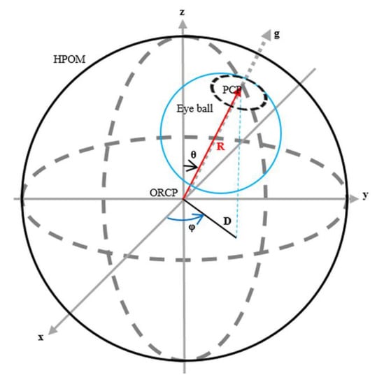
Figure 1.
Relationships between PCP and ORCP in Spherical Coordinates.
2.4. PPC Analysis
The pupil was observed as various elliptic shapes according to the gaze direction. It can be assumed to be a circle with zero eccentricity when pointed directly at the camera placed in front of the face [19]. Based on this, two prerequisites were set to estimate the 3D position of the PCP as follows:
- The pupil is a disk with zero eccentricity while located on the surface of the HPOM and being perpendicular to the g-axis.
- The xy-coordinate system of the camera and HPOM are parallel.
Based on the established premise, the three-dimensional position of the pupil is estimated by analysing the PPC data that includes various elliptic shapes depending on the gaze direction. When the gaze direction is changed while ϕ is fixed to 0, the HPOM observed by the camera can be represented by the x-z section shown in Figure 2. The shape of the pupil projected onto the camera is shown in Figure 3. When the gaze direction is perpendicular to the camera, θ becomes 0. The pupil disk is positioned as shown A in Figure 2. It is projected as a circle with zero eccentricity, as shown A in Figure 3. On the other hand, when the gaze direction is not perpendicular to the plane of the camera, the pupil disk is positioned as shown B in Figure 2. This is due to a three-dimensional rotational movement based on the ORCP as set out in the premise. Due to this, the three-dimensionally rotated and moved pupil disk is projected orthogonally to the camera, resulting in the elliptical shape shown B in Figure 3.
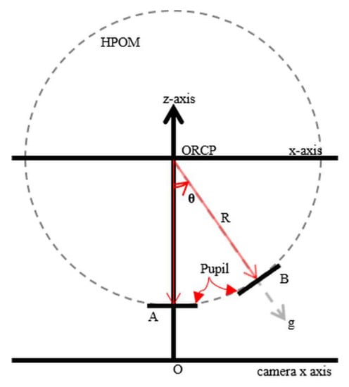
Figure 2.
Ellipse change principle of the pupil shown in the cross section of the x-axis and z-axis coordinate system.
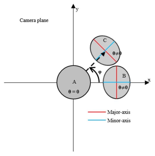
Figure 3.
Shape of PPC according to ϕ and θ.
If the gaze direction changes from position B shown in Figure 2 while θ is fixed, the PPC appears in the form of B being rotated along the z-axis relative to the ORCP, as shown C in Figure 3. Therefore, θ is the Rotation Angle of the Eye (RAE). This causes a change in the pupil’s size due to changes in the eccentricity of the PPC and a change in the distance along the z-axis. ϕ is the Rotation Direction Angle of the eye (RDA). This causes rotation of the PPC. In addition, it can be seen that the short axis of the elliptically-changed PPC is formed at the same angle as the RDA.
2.5. 3D Rotation of the Pupil Disc
Previously, the principle that the eccentricity and rotation of the PPC changes according to the RAE and RDA using HPOM, was analysed. Based on the results of this analysis, a three-dimensional Rotation Model of a Disk (RMD) was constructed to analyse the attitude of the pupil in three-dimensional space. RMD is a model used to observe the three-dimensional attitude of the eye using images captured by a camera that observes changes due to the rotation along each axis of the disk in an environment where the xy-coordinate system of the camera and the disk are synchronized, and a constant distance is maintained along the z-axis. When the disk is perpendicular to the z-axis of the camera, the initial attitude of the RMD is set and the attitude of the disk in 3D with respect to the centre point and the shape projected to the camera is analysed.
Figure 4a,b was obtained by adjusting the initial y-axis rotation angle setting the attitude of the RMD. In Figure 4a,b, the short axis lengths appears to be in inverse proportion to the rotation angle of the y-axis due to the relationship shown in Figure 5. It shows the disk attitude before and after y-axis rotation on the xz-plane, showing the formation principle for the diameters and of the disk projected on the camera. Since the disk is parallel to the camera plane in its initial attitude, the angle between the rotated disk and the camera plane is the same as the rotation angle of the disk. Therefore, the length of the diameter projected onto the camera plane when the rotational changes as much as θ occur can be calculated using Equation (3) based on a trigonometric function. In addition, the diameter of the disk’s tangent to the y-axis, where the rotation occurs, is the same as the diameter of the disk regardless of the size of the rotation angle. This appears as the long radius of the ellipse. Therefore, if it is possible to calculate , the short axis of the projected ellipse after a three-dimensional rotation change, and also , the long axis, (3) can be summarized with respect to the rotation angle of the disk, θ, and calculated using Equation (4).
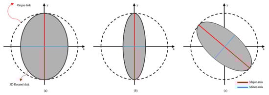
Figure 4.
Projected result as an ellipse onto the camera after a disk has rotated each axis. (a) The shape of the projected disk when the rotation of the y-axis occurs. (b) The shape of the projected disk when the rotation of the y-axis different magnitude from (a) occurs. (c) The shape of the projected disk when the rotation of the x-, y-, and z-axis are randomly.
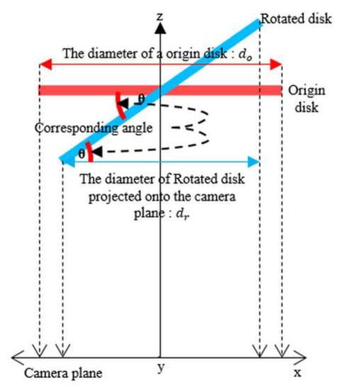
Figure 5.
Principle of the disk being projected onto an ellipse.
The length of the long axis is constant at even though θ, the rotation angle of the y-axis, varies. This is because there is no change in the distance between the camera and the z-axis in that part of the disk that was in contact with the y-axis at the point where the rotation occurred. Based on this, it was expected that the length of the long axis would always be constant even if rotation of the other axis occurred. To confirm this, the result was projected on the camera as each axis was rotated through all angles, as shown in Figure 4c. Despite the lengths of the short and long axes of the ellipse changing, as well as the angle formed with the x axis changing, the length of the long axis remains the same, i.e., .
By reflecting the RMD analysis to PPC changes according to attitude changes of the pupil disk that were analysed previously, the results can be interpreted according to our premise, as shown in Figure 6. In Figure 6, points O, P, and Q indicate the ORCP, PCP, and the position when a line is drawn perpendicular to the z-axis in the PCP, respectively. Point R is the position where the z-axis is met by a perpendicular line drawn parallel to the rotated pupil disk in PCP. Since the sum of the interior angles of a right triangle is always 180 degrees, the angle of QRP can be calculated using Equation (4). Using the same principle, it can be seen that the rotation angle θ of the pupil disk is the same as the RAE. Therefore, if lengths of the short axis and the long axis of the PPC are known, the RAE can be calculated according to Equation (5). Thus, the three-dimensional position of the PPC can be approximated using the centre point of the PCP and the RAE.

Figure 6.
Relationship between the RAE of HPOM and the rotation angle of the pupil.
2.6. Presumptive Background of HPOM
The three-dimensional position of the pupil could be approximated by using PPC analysis of the previously observed pupil as an ellipse. When the HPOM is a sphere, the distance between the ORCP and the PCP is constant despite any changes in the 3D position of the PCP. Based on this, the HPOM can be reconstructed through the process of calculating the position of the ORCP and the radius of the HPOM using the 3D position of the PCP.
2.6.1. ORCP Inference
When the HPOM is a sphere, the three-dimensional position of the PCP according to how gaze direction changes is reflected on the surface of the sphere orbit centred on the ORCP. Figure 7a shows positions of the ORCP and PCP in 3D space resulting from randomly acquiring n PCPs () as the gaze direction changes. Since the distance between the ORCP and PCP is always constant, the position where the ORCP can exist can be expressed as shown in Figure 7b. This is done with respect to each point P and is expressed by Equation (6) with a sphere equation. Spheres centred at each point, P, intersect each other. All spheres intersect at the ORCP.
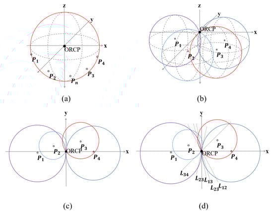
Figure 7.
(a) The spherical orbital formed by PCP. (b) Candidate positions of the centre point of a spherical orbit located at a certain distance from each PCP. (c) Candidate positions obtained from the z-axis position of ORCP. (d) Lines passing through intersections of circles.
The intersection of all spheres centred on each point P in 3D space can be obtained by considering the intersecting surfaces of the spheres. However, since we can’t directly acquire the z-axis position of the PCP, it is difficult to estimate the ORCP despite calculating the equation of the three-dimensional plane where the spheres meet. In order to overcome this, the variables related to the z-axis position in (6) are summarized as shown in Equation (8) using Equation (7). This shows the positional relationship between the ORCP and PCP on the xy-plane in the spherical coordinate system. The transformation process from Equation (6) to Equation (8) is described as the process of calculating the xy section of the sphere centred for each point P at the z-axis position of the ORCP, the result of which are shown in Figure 7c. By Equation (8), the position where ORCP can exist around each point P is limited to a circle on the xy-plane. This can be expressed as the equation of a circle (Equation (9)). Circles centred at each point P have radii proportional to RAE. All circles intersect at ORCP and have a maximum of two intersections with each of the other circles. A circle with a different RDA always intersects with each other only at the ORCP regardless of the size of their RAE. For this reason, at least three circles centred on the point P are required to estimate the ORCP.
The ORCP where all circles intersect can be obtained by considering a straight line passing through that intersection point where each circle intersects the others. Figure 7d shows a straight line (Lnm) passing through the intersection of circles centered on points Pn and Pm. All straight lines intersect at one point and all circles intersect at the same point. Based on this, in order to calculate a straight line passing through the intersection point of the circles, Equation (9) of the circle centred on each point P is combined and arranged as shown in Equation (10). By using Equation (10), the radius of the unknown HPOM can be eliminated. However, the calculation result of Equation (10) is arranged in the form of a straight-line equation to obtain Equation (11) when the difference of the constant K in Equation (10), i.e., the coefficient of the quadratic term, is 0. On the other hand, in the form of the new circle equation shown in Equation (12), when K is not 0, this resolves. Since at least one of the intersection points of the two circles is always an ORCP, the equation of the newly calculated circle also forms an intersection point in the ORCP. Therefore, equations of all the circles, newly obtained through the simultaneous process, are divided and normalized by K in Equation (11), which gives the coefficient of each quadratic term. When equations of the normalized circle are simultaneously processed, the quadratic term is eliminated, and all can be arranged in the equation of a straight line (Equation (11)). Finally, the ORCP estimation is completed through the process of finding intersections of all the obtained straight lines. In order to find the intersections of all straight lines, these line equations are divided into a coefficient term, an unknown term, and a constant term. They can be arranged, as shown in Equation (13), as a determinant. Since the unknown term is the position on the xy-plane of the ORCP that is to be estimated, the ORCP can finally be calculated by solving Equation (14) after organizing for the unknown term by finding the inverse matrix for the constant term. The coefficient matrix that is expressed in Equation (13) is not a square matrix because of the number of lines for ORCP estimation is always greater than 2. Thus, the inverse matrix cannot be calculated using a general method. However, the pseudo-inverse matrix with similar functions to the inverse matrix can be considered. A pseudo-inverse calculation is an operation that can be used for all types of matrices and generalizes the inverse matrix operation of the invertible matrix. It can be applied to an invertible matrix and can be carried out using a Singular Value Decomposition (SVD) [32]. The coefficient matrix in Equation (13) is an invertible matrix because of every line for estimating the ORCP are crossed at a point. In conclusion, the ORCP can be calculated using a pseudo-inverse.
2.6.2. HPOM Radius Acquisition
The position of the ORCP on the xy-plane was calculated using the previously approximated position of the PCP. All PCPs centred on the acquired ORCP satisfied Equation (2) in the xy-plane as shown in Figure 8. The distance between ORCP and PCP on the xy-plane showed the same change as the sine wave according to the change in RAE. The maximum distance was equal to the radius of HPOM when RAE was 90 degrees. Based on this, the approximate three-dimensional position of the PCP can be reflected in Equation (2) and summarized as in Equation (15). The radius of the HPOM can be finally obtained by solving Equation (16), which is obtained the pseudo-inverse matrix of the coefficient term.
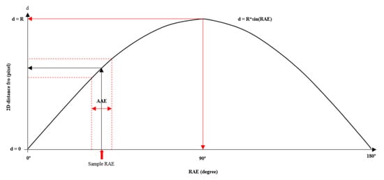
Figure 8.
Distance in xy-plane of ORCP and PCP according to RAE.
2.7. HPOM Fitting
The accuracy of the HPOM estimated according to the proposed theory is proportional to the error of the RAE obtained by analysing the PPC. To improve accuracy and stability, HPOM fitting is performed using the method proposed in this paper on the RANdom SAmple Consensus (RANSAC) published by Fischler, Martin A. and Robert C. Bolles [33]. The RANSAC method has a feature of repeatedly performing mathematical model estimation by randomly selecting the model Estimation Sample (ES) from the Total Sample (TS) and deriving an optimal result. As a result, even if the TS contains error samples, it shows high accuracy. However, there is a disadvantage in that the computational load is large in proportion to the number of TSs and ESs. Therefore, it is necessary to set the appropriate number of TS and ES to minimize the computational load with a good performance to derive an optimal model.
HPOM fitting repeats the hypothesis and verification steps according to the sequence shown in Figure 9. In the hypothesis stage, ES is randomly selected from TS and HPOM is estimated according to the proposed theory. The number of straight lines that can be calculated in the ORCP estimation process is proportional to the number of ES. Therefore, when the ORCP is estimated using many samples, an equation of a straight line with the same slope can be obtained. Lines with the same slope may cause high computational load and errors because of the innumerable intersections with other lines that appear. Hence, it is necessary to consider the slope in the process of calculating the equation of the straight line. Minimum Difference of Gradient (MDG) is used as the variable to exclude equations of straight lines that have the same slope. When the difference between the slope of the newly calculated line and the slope of the previously calculated line exceeds the MDG, it is used for the ORCP estimation. If the MDG is set to ±1 degree, the maximum number of straight lines that can be obtained is 359, even if there are a huge number of samples.
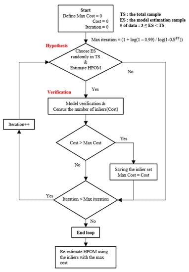
Figure 9.
Process of RANSAC to estimate HPOM.
In the verification step, error determination is carried out. TS samples satisfying the HPOM estimated in the hypothesis step are classified as inliers. The quantity of these is acquired as a cost. Error determination is performed by examining the distance on the xy-plane of the ORCP using determination of the object sample and using the RAE of the determined object sample found in Equation (2). However, since the shape of the pupil observed by the camera might be distorted according to the characteristics of the lens, an error in the RAE may occur. Therefore, the Allowable Angle Error (AAE) is reflected by a range variable that sets the allowable error range for the distance in two-dimensional coordinates of the sample being judged. After that, the measured error of the sample being judged is calculated according to Equation (2). This result is then compared and classified as an inlier if it is smaller than the AAE and as an outlier if it is bigger than the AAE. If the cost obtained by error determination is large compared to the maximum cost, samples classified as inliers are stored. This is done so the larger the cost obtained through error determination, the more similar the estimated HPOM is to the actual HPOM. This process is repeated and the optimal HPOM is re-estimated using the inlier obtained when the cost is at its maximum.
2.8. Experiments
The purpose of the experiment we conducted was to verify the validity of the theory proposed in this paper, and was also to analyse the influence of variables in the fitting process. Distance units are expressed in pixels because the pupil is acquired using the camera where distance is measured by pixels. We retained the unit of pixels in order to avoid the complication of a separate conversion process.
The experiments build on the procedure in Section 2.7 and are simulated by generating virtual data on the assumption that data is obtained based on the suggested environment in Section 2.2. The number of ES refers to the number of samples used to estimate the initial model in the hypothesis stage of the RANSAC method. This number of samples determines processing time, accuracy, and flexibility. In the experiment, space was formed so the x, y, and z-axes were all 500 pixels in size. The simulation data used was acquired using 3D rotation of the pupil disc. The rotating centre point of a pupil disc was set to be the centre of coordinate space, while the distance from the disc centre to the space centre was set to 250 pixels. The pupil disc radius was set to 50 pixels. A total of 100 samples were obtained for HPOM estimation, this was done by converting random position coordinates to positions of the x- and y-axes while RAE was recorded using 3D rotations of the pupil disc. In addition, a dataset of 200 TSs with an inlier to outlier ratio of 1:1 was constructed by randomly generating 100 pieces of noise data, as shown in Figure 10a. Figure 10b shows the distances on the xy-plane from the dataset along with the distribution of the RAE.
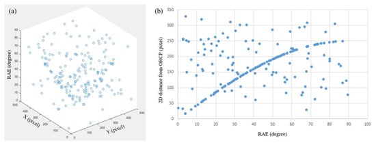
Figure 10.
(a) 3D dataset distribution diagram. (b) Data set distribution diagram expressed in RAE and the distance between ORCP and each data on the xy-plane.
In order to analyse the performance of our method according to independent variables, such as the number of ESs, the values of the AAEs and MDGs, the experiment was performed by setting the processing time, location and distribution of the average ORCP, the radius of the HPOM, and the max cost as the dependent variables. The experiment was carried out over two sessions. In the first session the experiment was verified the validity of the proposed method and repeated 200 times while gradually increasing the ES as the independent variable from 3 to 14 in order to check the accuracy of the HPOM estimated as ES changed. AAE is the tolerance range of RAE, which does not provide flexible estimation of the model if set to an excessively small range. On the other hand, if AAE is set to a wide range, the accuracy of the model may decrease. MDG is a variable for the purpose of reducing the excessive load applied to the system when estimating the HPOM. In order not to affect the first experiment control variables, AAE was fixed at ±5 degrees and MDG was fixed at ±0 degree. The results were analysed after performing a total of five sets of these experiments.
In the second session, the ES was fixed, reflecting results of the first experiment, to confirm the model’s performance according to changes in the AAE and MDG. Afterwards, the experiment was repeated 200 times while varying the AAE from 1 degree to 5 degrees in 1-degree increments and varying the MDG from 0 to 5 degrees, also by 1 degree increments.
3. Results
The experiment was carried out using Visual studio 2017 supplied by Microsoft (Washington, DC, USA) and Open Source Computer Vision (OpenCV) supplied by Intel (Los Angeles, CA, USA), an image processing library, on a PC equipped with an Intel Core i7-7700k CPU manufactured in California of United States and SAMSUNG 64G RAM manufactured in Suwon-si of Korea on which the programs were configured and the experiments conducted. The OpenCV library includes various image processing functions and also provides specialized matrix operation functions.
Table 1 shows the results from the first experiment. The HPOM could not be calculated successfully when the ES was 3 during these experiments. Therefore, the results were analysed after excluding results when the ES was set to 3. On average the processing time for each experiment was about 80 s when the ES was less than 10. The standard deviation was about ±5 s. When the ES was 14, about 470 s were required, with a standard deviation of ± 15 s. As the ES increased, the processing time gradually increased. However, this did not affect the average cost. The estimated ORCP remained constant regardless of the ES. In Table 1, the distribution of the ORCP, displayed as a distance, shows a tendency to decrease as ES increases, but when the ES exceeds a certain number, the processing time and distribution both increase.

Table 1.
Performance of HPOM estimation according to ES.
The second experiment was carried out with the ES set to 7, reflecting the average performance from the first experiment. Table 2 shows the results from the second experiment. The processing time was over 1 min when the MDG was set to 0 degrees, while it was less than 1 s when the MDG was above 1 degree. Furthermore, the average of the ORCP and the radius of the HPOM remained constant within a 1-pixel range. The distribution of the ORCP was most concentrated when the MDG was set to 0, independent of the AAE. However, the distribution of the ORCP was irregular when MDG was over 0. The average cost was found to be directly proportional to the AAE without being affected by changes to the MDG.
Table 2.
Performance of HPOM estimation according to AAE and MDG.
4. Discussion
We confirmed in the first experiment that the HPOM can be estimated by using the proposed method and the ES had an effect on the HPOM estimation process. The minimum amount of accurate data required for the estimation of HPOM was found to be three in this paper. However, when the ES was three, the estimation of the HPOM failed. This is due to the random sampling characteristics of RANSAC and the fact that half of the TS consists of error data. The RANSAC method relies on probability because it randomly selects a sample in order to estimate the best fit model. Therefore, the probability of estimating a suitable model is determined in proportion to the error data ratio and the number of estimation iterations. When, the ES is 3, the probability that all data selected for estimating the HPOM does not contain errors is less than 1.3%. The number of iterations is also determined by the ES. The maximum number of iterations when ES is 3 is 35. The means that HPOM estimation was impossible when the ES was 3, as the probability of estimating the HPOM accurately is less than 1.3%, and this is unlikely to occur once over the maximum 35 iterations. Consequently, HPOM estimation is almost impossible according to the probabilities at play when the ES is 3. In addition, when the ES was set excessively high, the processing time increased while the accuracy decreased. The increase in processing time is an expected result of the ORCP inference because the number of straight lines generated is proportional to the ES. Increasing the ES also causes a growth in the possibility an error is included in the data sample. Therefore, the ORCP of the estimated HPOM has a wide spread, as the error proportion of the samples included in the ES increases. Conversely, when the ES is minimized, the ORCP distribution becomes wide because the mathematical model of the initial HPOM is only weakly acquired in the RANSAC process. In summary, an increase in the number of ESs leads to an increase in processing time of whole process, and the error sample ratio of ES, but increases the accuracy of ORCP and radius accuracy of HPOM. In addition, comparing the result of ES is 10 and 14 in Table 1, an unnecessary number of ESs may cause a decrease in performance. Therefore, it can be said that the model estimation is more flexible. Consequently, it is vital to set an appropriate ES in order to calculate the HPOM accurately.
The second experiment was performed by choosing the ES that showed average performance in the first experiment, i.e., the ES was set to 7, as the ES was set to the average needed in order to confirm the general tendencies of varying the AAE and MDG on performance. It was found that processing time and cost both had a tendency to increase as the AAE was increased. The cost indicates the number of samples required in order to estimate an optimized HPOM. The samples used for an optimized HPOM estimation were selected in the RANSAC verification process based on the range of the AAE. Furthermore, the processing time is unconditionally influenced by the cost. This is because a cost increase leads to an increasing number of straight lines being used in the ORCP inference section. Therefore, the cost and the processing time are subordinate to the AAE. On the other hand, the effect of the AAE on the accuracy of the HPOM cannot be confirmed owing to the characteristics of RANSAC in that the estimation process is repeated until an optimal model is found. The MDG affects the accuracy of the HPOM and processing time. A processing time of over 60 s is seen when the MDG is set to 0. On the other hand, when the MDG is greater than 0, the processing time is greatly reduced to under 1 s. This result means MDG accurately satisfied our goal of decreasing the processing time. The accuracy of the HPOM is almost constant when the MDG is set to 0, regardless of the AAE used. However, the accuracy of the HPOM is irregular when the MDG is not 0. Setting the MDG to greater than 0 seems to reduce the accuracy of the HPOM estimation. This result is thought to be the result of a lack of discernment in the method that uses the MDG. The MDG only compares the angle of straight lines without considering the intersection point in the ORCP inference section. Thus, lines passing through the ORCP with the same slope are disregarded if lines that do not pass through the ORCP are first classified as inliers. Therefore, the accuracy of the HPOM becomes irregular regardless of the MDG when the MDG is greater than 0. In conclusion, the MDG effectively reduces the processing time, but brings the penalty of reduced HPOM accuracy.
The accuracy of the proposed method is reliant on the RANSAC method. As such, our approach relies on the quality and amount of data used for HPOM estimation. In particular, the amount of data from repeatedly photographing the face may produce satisfactory estimates, while camera performance affects the quality of data that can be collected. This is because when the shape of the pupil cannot be accurately identified, pupil shape analysis to estimate HPOM becomes impossible. In addition, the proposed method needs at least three images with different eye-gaze directions. This condition is caused by the characteristic of the RANSAC method. The RANSAC method is a technique for approximating the expected model that can explain the entire data using a small amount of data. This means that the RANSAC method has an advantage because the model can be approximated even though the data contains errors. However, in the hypothesis step of the RANSAC method, model approximation is not possible if the data consist only of errors or if all data are identical. This means that the data have not linearity or does not match to the expect model. Therefore, the proposed method has a same weakness of the RANSAC method.
On the other hand, the proposed method can estimate the HPOM regardless of the camera’s distance from the face as long as it can acquire the pupil shape. In addition, the consumption time is very short at 0.4 s. In other words, our method can respond in real time even when the subject being monitored moves. Incidentally, in this paper, we limited HPOM to a sphere, but later research is planned where this will be expanded to ellipsoids. Moreover, we plan to conduct further research with the aim of improving accuracy.
5. Conclusions
In conclusion, in this paper we present a novel pre-processing method for eye-gaze tracking based on a camera recording the front of a subject’s face that works regardless of the distance from the eye to the camera. The proposed method simplified the rotational movement of the eyeball observed in the camera as RMD analysis. The relationship between the pose of the pupil in 3D space and the PPC was analysed using RMD analysis. Based on this, the three-dimensional position and pose of the pupil could be approximated only with the information of the PPC. Finally, the HPOM could be estimated using the RANSAC method. The proposed method is performed in a short time of less than 1 s, and it is possible to obtain HPOM with an error of less than 1 pixel in ORCP and radius performance. The proposed method not only finds the centre of rotation of the eyeball, which was a problem in previous studies, but also improves eye tracking method by simplifying the 3D space into a 2D space. The validity and performance of HPOM estimation were confirmed by the proposed method through a series of experiments. In addition, the execution time to achieve this was less than 1 s, enabling adaptive HPOM estimation that responds to user movements in real time. Moreover, even when the pupil was photographed from a distance, the HPOM could be estimated. As such, we believe that our method will serve as the basis for development of single camera eye-tracking solutions as the need for this grows due to new technologies that depend on this ability.
Author Contributions
Conceptualization, S.L.; methodology, S.L.; software, S.L.; validation, S.L., J.J. and D.K.; formal analysis, S.L.; investigation, S.L. and D.K.; writing—original draft preparation, S.L.; writing—review and editing, J.J.; supervision, S.K.; project administration, J.J. All authors have read and agreed to the published version of the manuscript.
Funding
This research received no external funding.
Institutional Review Board Statement
Not applicable.
Informed Consent Statement
Not applicable.
Data Availability Statement
Not applicable.
Acknowledgments
This work was supported and funded by the Dongguk University Research Fund of 2022(S-2022-G0001-00064).
Conflicts of Interest
The authors declare no conflict of interest.
References
- Lobmaier, J.S.; Tiddeman, B.P.; Perrett, D.I. Emotional expression modulates perceived gaze direction. Emotion 2008, 8, 573. [Google Scholar] [CrossRef] [PubMed] [Green Version]
- Abbasi, J.A.; Mullins, D.; Ringelstein, N.; Reilhac, P.; Jones, E.; Glavin, M. An Analysis of Driver Gaze Behaviour at Roundabouts. IEEE Trans. Intell. Transp. Syst. 2021, 23, 8715–8722. [Google Scholar] [CrossRef]
- Tresanchez, M.; Pallejà, T.; Palacín, J. Optical Mouse Sensor for Eye Blink Detection and Pupil Tracking: Application in a Low-Cost Eye-Controlled Pointing Device. J. Sens. 2019, 2019, 3931713. [Google Scholar] [CrossRef]
- Klaib, A.F.; Alsrehin, N.O.; Melhem, W.Y.; Bashtawi, H.O. IoT smart home using eye tracking and voice interfaces for elderly and special needs people. J. Commun. 2019, 14, 614–621. [Google Scholar] [CrossRef]
- Martinez-Conde, S.; Macknik, S.L. From exploration to fixation: An integrative view of Yarbus’s vision. Perception 2015, 44, 884–899. [Google Scholar] [CrossRef] [Green Version]
- Vodrahalli, K.; Filipkowski, M.; Chen, T.; Zou, J.; Liao, Y.J. Predicting Visuo-Motor Diseases from Eye Tracking Data. Pac. Symp. Biocomput. 2022, 2021, 242–253. [Google Scholar]
- Baba, T. Detecting Diabetic Retinal Neuropathy Using Fundus Perimetry. Int. J. Mol. Sci. 2021, 22, 10726. [Google Scholar] [CrossRef]
- Qian, K.; Arichi, T.; Price, A.; Dall’Orso, S.; Eden, J.; Noh, Y.; Rhode, K.; Burdet, E.; Neil, M.; Edwards, A.D.; et al. An eye tracking based virtual reality system for use inside magnetic resonance imaging systems. Sci. Rep. 2021, 11, 16301. [Google Scholar] [CrossRef]
- Mystakidis, S. Metaverse. Encyclopedia 2022, 2, 486–497. [Google Scholar] [CrossRef]
- Sipatchin, A.; Wahl, S.; Rifai, K. Eye-tracking for clinical ophthalmology with virtual reality (vr): A case study of the htc vive pro eye’s usability. Healthcare 2021, 9, 180. [Google Scholar] [CrossRef]
- DuTell, V.; Gibaldi, A.; Focarelli, G.; Olshausen, B.A.; Banks, M.S. High-fidelity eye, head, body, and world tracking with a wearable device. Behav. Res. Methods 2022, 1–11. [Google Scholar] [CrossRef] [PubMed]
- Chang, C.K.; Liao, J.Y.; Chen, D.C.; Yeh, F.M.; Chang, S.T.; Hsu, C.K. Binocular 3D Vision Fusion Measurement Technique. In Proceedings of the International Symposium on Intelligent Signal Processing and Communication Systems (ISPACS), Hualien, Taiwan, 16–19 November 2021; IEEE: Piscataway, NJ, USA; pp. 1–2. [Google Scholar]
- Mou, X.; Mou, T. Measurement of AR Displays in Positioning Accuracy. In Proceedings of the SID Symposium Digest of Technical Papers, Oregon, Portland, 18–21 May 2022; Wiley: Hoboken, NJ, USA; Volume 53, pp. 1261–1263. [Google Scholar] [CrossRef]
- Ryu, J.; Lee, M.; Kim, D.H. EOG-based eye tracking protocol using baseline drift removal algorithm for long-term eye movement detection. Expert Syst. Appl. 2019, 131, 275–287. [Google Scholar] [CrossRef]
- Khaldi, A.; Daniel, E.; Massin, L.; Kärnfelt, C.; Ferranti, F.; Lahuec, C.; Seguin, F.; Nourrit, V.; de Bougrenet de la Tocnaye, J.-L. A laser emitting contact lens for eye tracking. Sci. Rep. 2020, 10, 14804. [Google Scholar] [CrossRef] [PubMed]
- Mastrangelo, A.S.; Karkhanis, M.; Likhite, R.; Bulbul, A.; Kim, H.; Mastrangelo, C.H.; Hasan, N.; Ghosh, T.A. A low-profile digital eye-tracking oculometer for smart eyeglasses. In Proceedings of the 2018 11th International Conference on Human System Interaction (HSI), Gdańsk, Poland, 4–6 July 2018; IEEE: Piscataway, NJ, USA, 2018. [Google Scholar]
- Zhang, W.; Zhang, T.N.; Chang, S.J. Eye gaze estimation from the elliptical features of one iris. Opt. Eng. 2011, 50, 047003. [Google Scholar] [CrossRef]
- Baek, S.J.; Choi, K.A.; Ma, C.; Kim, Y.H.; Ko, S.J. Eyeball model-based iris center localization for visible image-based eye-gaze tracking systems. IEEE Trans. Consum. Electron. 2013, 59, 415–421. [Google Scholar] [CrossRef]
- Karakaya, M.; Barstow, D.; Santos-Villalobos, H.; Thompson, J.; Bolme, D.; Boehnen, C. Gaze estimation for off-angle iris recognition based on the biometric eye model. Biometric and Surveillance Technology for Human and Activity Identification X. Int. Soc. Opt. Photonics 2013, 8712, 83–91. [Google Scholar]
- Qi, Y.; Wang, Z.L.; Huang, Y.A. non-contact eye-gaze tracking system for human computer interaction. In Proceedings of the 2007 International Conference on Wavelet Analysis and Pattern Recognition, Beijing, China, 2–4 November 2007; IEEE: Piscataway, NJ, USA; Volume 1, pp. 68–72. [Google Scholar]
- Hennessey, C.; Noureddin, B.; Lawrence, P. A single camera eye-gaze tracking system with free head motion. In Proceedings of the 2006 Symposium on Eye Tracking Research and Applications Symposium (ETRA), San Diego, CA, USA, 27–29 March 2006; Association for Computing Machinery (ACM): New York, NY, USA; pp. 87–94. [Google Scholar]
- Koshikawa, K.; Sasaki, M.; Utsu, T.; Takemura, K. Polarized Near-Infrared Light Emission for Eye Gaze Estimation. In ACM Symposium on Eye Tracking Research and Applications; Association for Computing Machinery (ACM): New York, NY, USA, 2020; pp. 1–4. [Google Scholar]
- Beymer, D.; Flickner, M. Eye gaze tracking using an active stereo head. In Proceedings of the 2003 IEEE Computer Society Conference on Computer Vision and Pattern Recognition, Madison, WI, USA, 18–20 June 2003; Volume 2, p. II-451. [Google Scholar]
- Via, R.; Hennings, F.; Fattori, G.; Fassi, A.; Pica, A.; Lomax, A.; Weber, D.C.; Baroni, G.; Hrbacek, J. Noninvasive eye localization in ocular proton therapy through optical eye tracking: A proof of concept. Med. Phys. 2018, 45, 2186–2194. [Google Scholar] [CrossRef]
- Chen, J.; Ji, Q. 3D gaze estimation with a single camera without IR illumination. In Proceedings of the 2008 19th International Conference on Pattern Recognition, Tampa, FL, USA, 8–11 December 2008; pp. 1–4. [Google Scholar]
- Reale, M.; Hung, T.; Yin, L. Viewing direction estimation based on 3D eyeball construction for HRI. In Proceedings of the 2010 IEEE Computer Society Conference on Computer Vision and Pattern Recognition-Workshops, San Francisco, CA, USA, 13–18 June 2010; pp. 24–31. [Google Scholar]
- Wen, Q.; Bradley, D.; Beeler, T.; Park, S.; Hilliges, O.; Yong, J.; Xu, F. Accurate Real-time 3D Gaze Tracking Using a Lightweight Eyeball Calibration. Comput. Graph. Forum 2020, 39, 475–485. [Google Scholar] [CrossRef]
- Utsu, T.; Takemura, K. Remote corneal imaging by integrating a 3D face model and an eyeball model. In Proceedings of the 11th ACM Symposium on Eye Tracking Research & Applications, Denver, CO, USA, 25–28 June 2019; pp. 1–5. [Google Scholar]
- Dierkes, K.; Kassner, M.; Bulling, A. A fast approach to refraction-aware eye-model fitting and gaze prediction. In Proceedings of the 11th ACM Symposium on Eye Tracking Research & Applications, Denver, CO, USA, 25–28 June 2019; pp. 1–9. [Google Scholar]
- Demer, J.L.; Robert, A.C. Translation and eccentric rotation in ocular motor modeling. Prog. Brain Res. 2019, 248, 117–126. [Google Scholar]
- Chen, J.; Venkataraman, K.; Bakin, D.; Rodricks, B.; Gravelle, R.; Rao, P.; Ni, Y. Digital camera imaging system simulation. IEEE Trans. Electron Devices 2009, 56, 2496–2505. [Google Scholar] [CrossRef]
- Golub, G.; Kahan, W. Calculating the singular values and pseudo-inverse of a matrix. J. Soc. Ind. Appl. Math. Ser. B Numer. Anal. 1965, 2, 205–224. [Google Scholar] [CrossRef]
- Fischler, M.A.; Bolles, R.C. Random sample consensus: A paradigm for model fitting with applications to image analysis and automated cartography. Commun. ACM 1981, 24, 381–395. [Google Scholar] [CrossRef]
Publisher’s Note: MDPI stays neutral with regard to jurisdictional claims in published maps and institutional affiliations. |
© 2022 by the authors. Licensee MDPI, Basel, Switzerland. This article is an open access article distributed under the terms and conditions of the Creative Commons Attribution (CC BY) license (https://creativecommons.org/licenses/by/4.0/).