
Robust Malware Family Classification Using Effective Features and Classifiers

 ,
,
Abstract
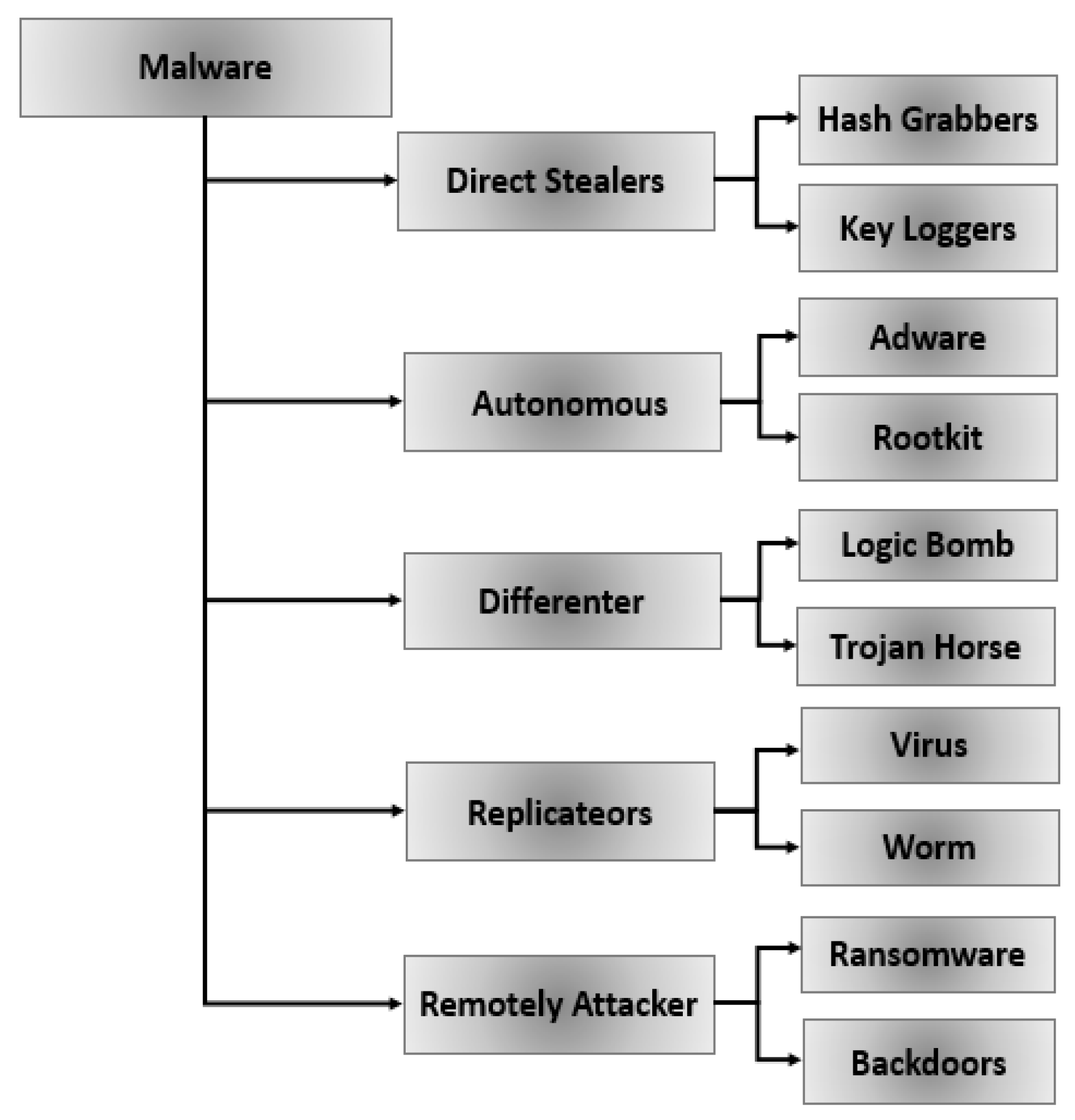
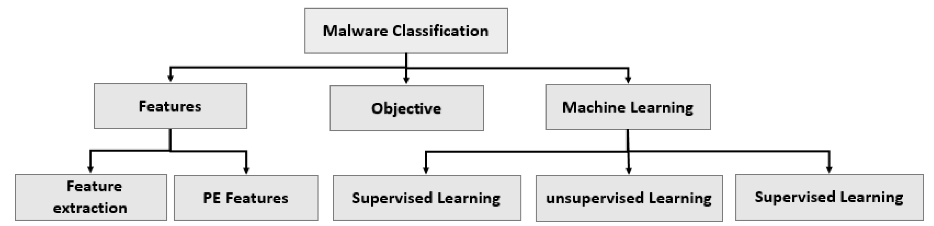
:1. Introduction
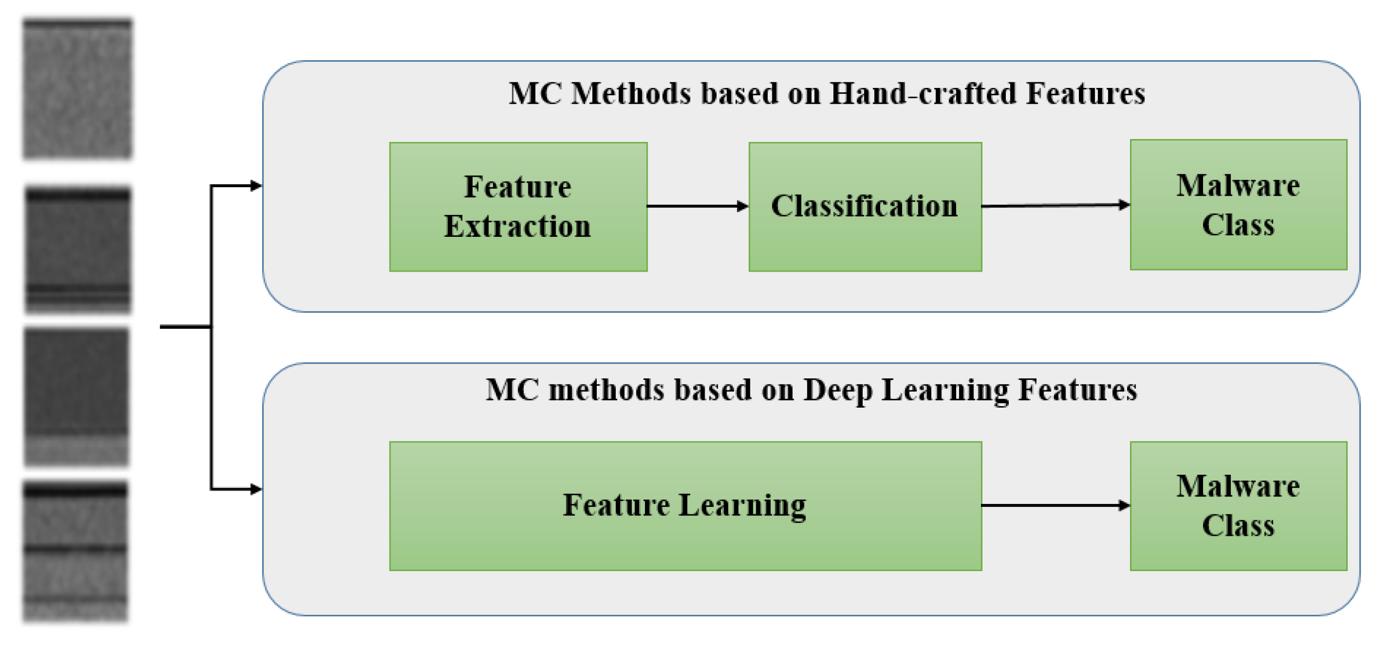
- Using the Tamara and deep methods, feature vectors are extracted in order to propose an effective malware classification method.
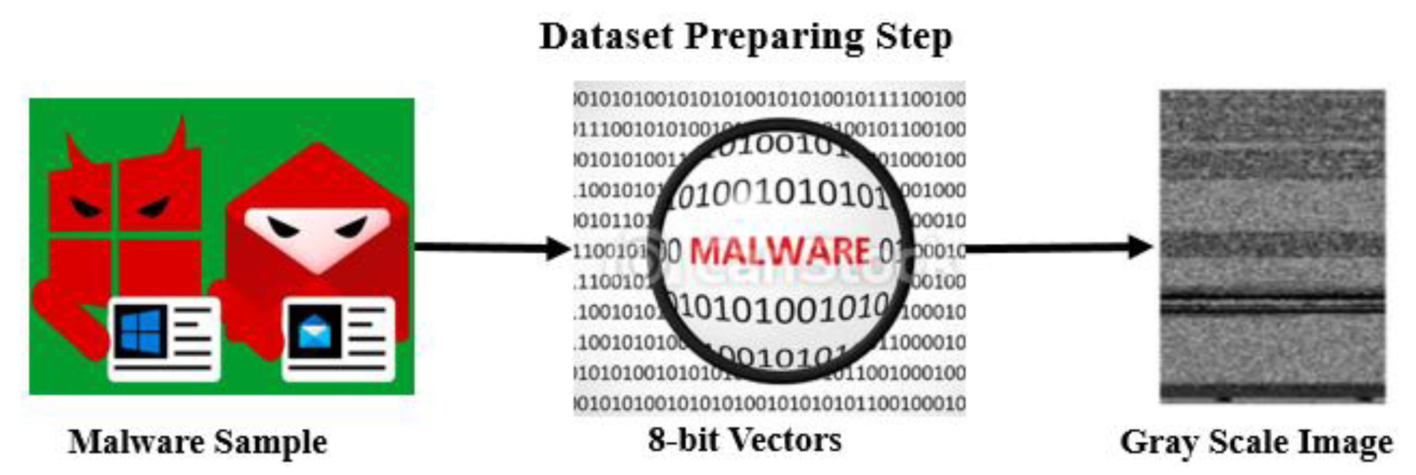
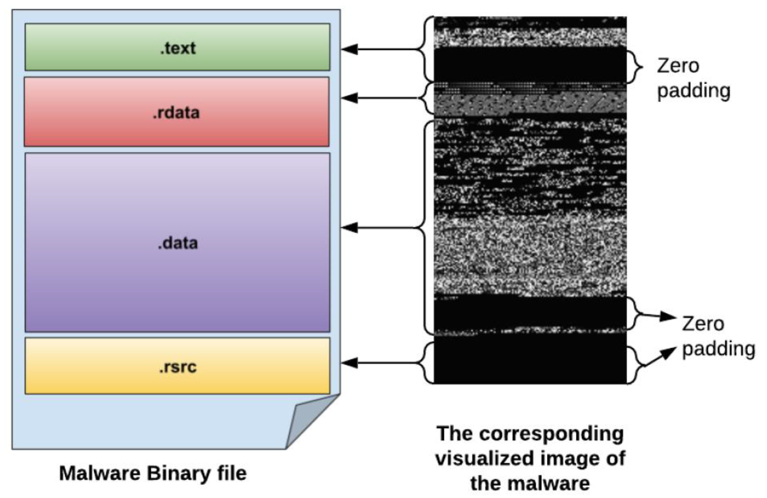
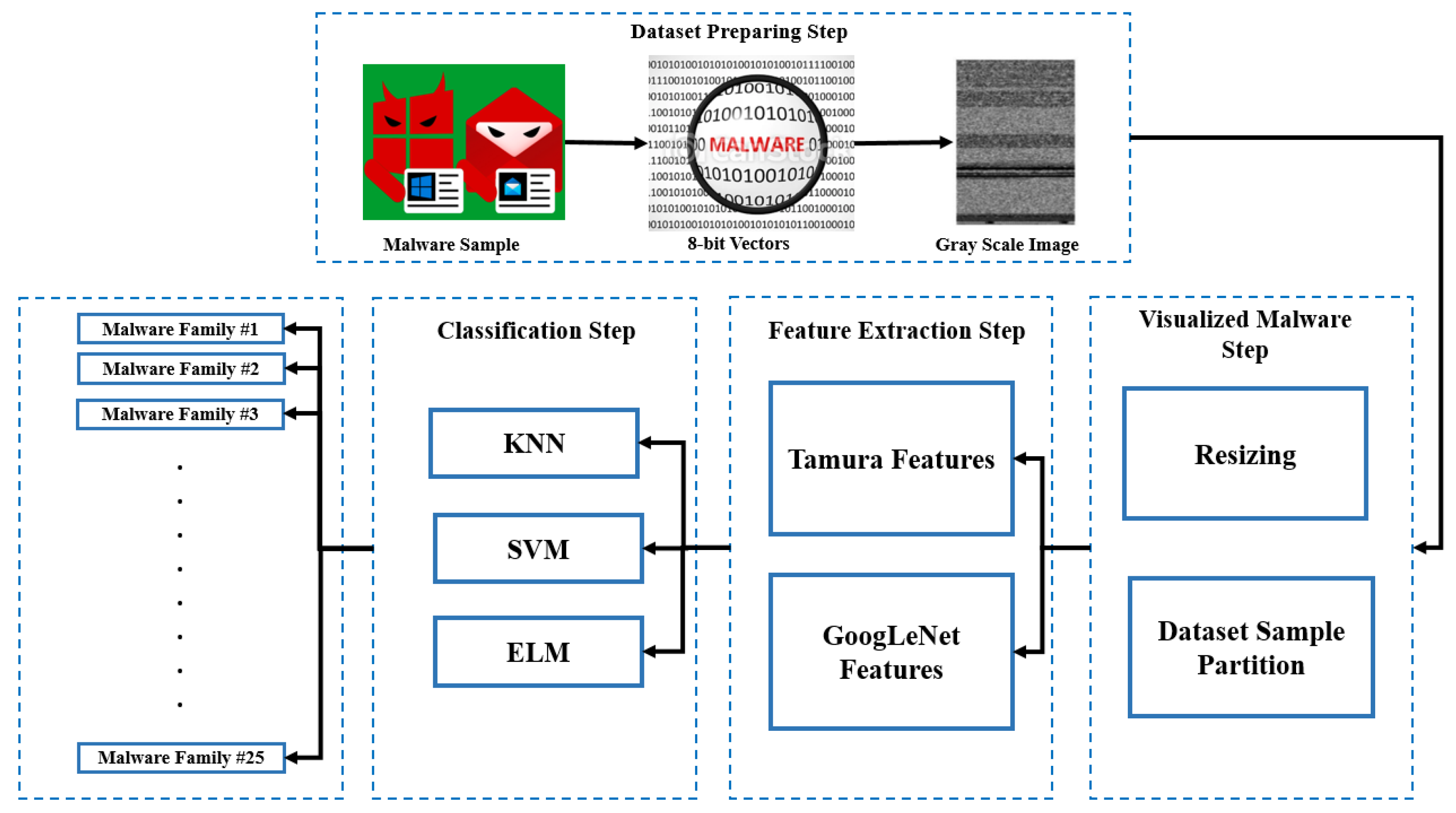
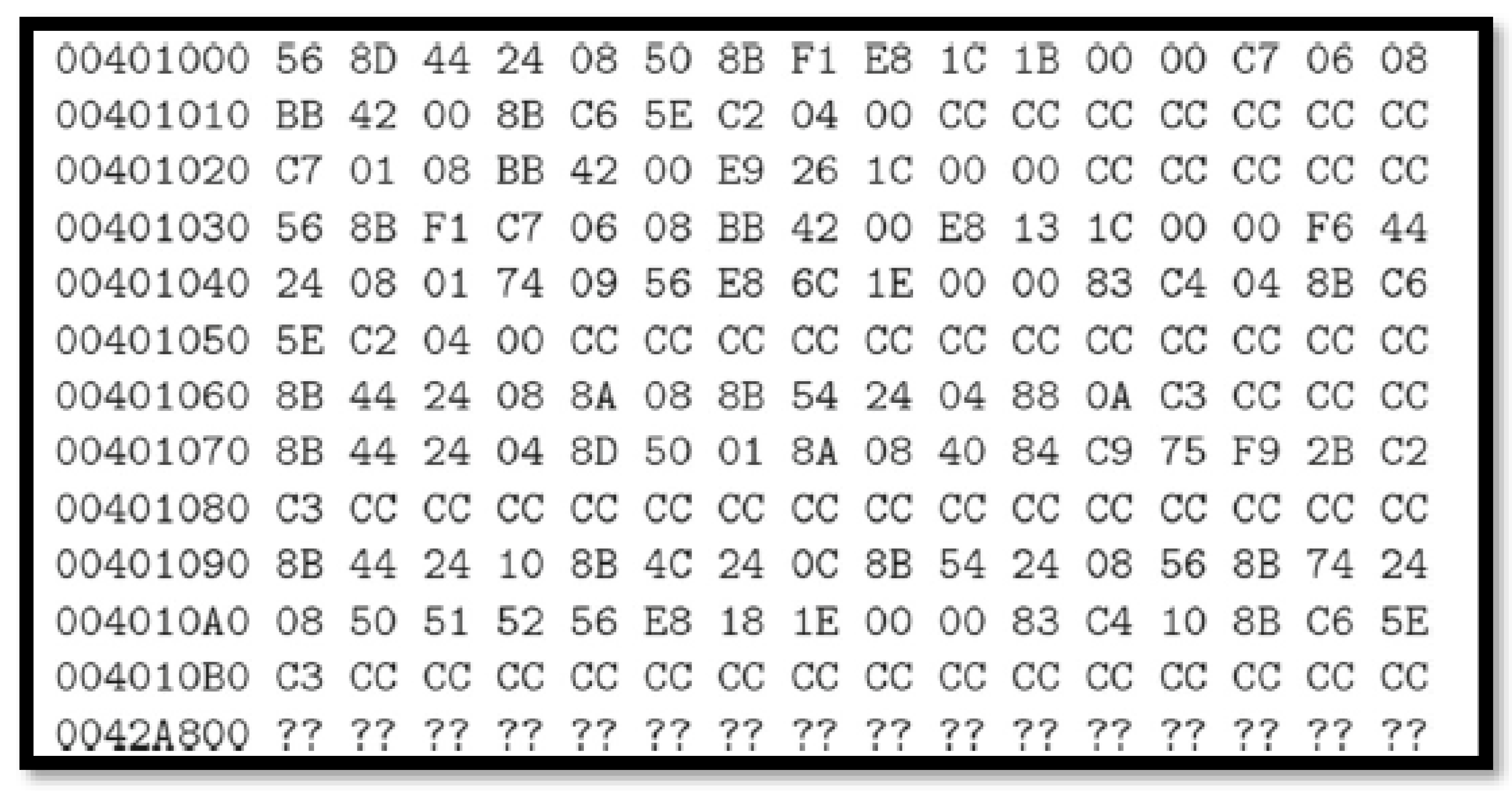
- It is proposed to use a malware visualization technique that produces grayscale graphics by converting binary files into 8-bit vectors.
- Classify malware with a visual component that employs a pre-trained CNN model that can identify visual malware samples without the need for features engineering.
- Using optimized CNN models to operate correctly on 9339 photos of 25 different malware families comprising eight distinct malware kinds.
- Seeking to establish a CNN model that can correctly classify malware using unbalanced dataset (e.g., Malimg dataset).
2. Related Works
3. Multiple Features
3.1. Tamura Feature
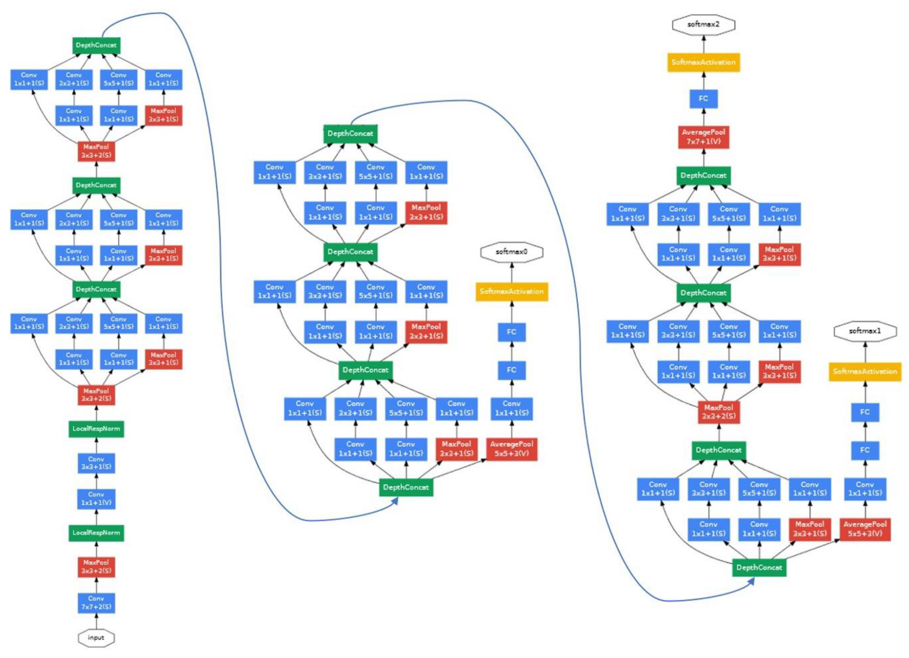
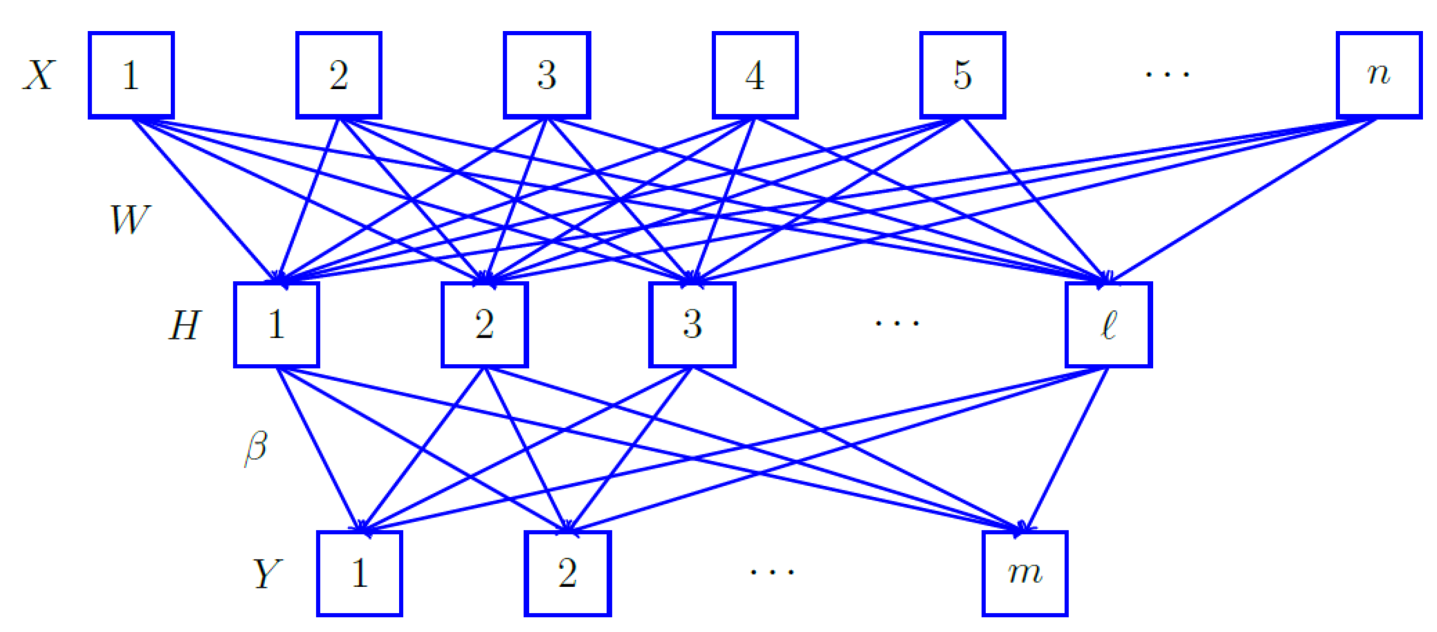
3.2. GoogleNet Deep Feature
4. The Proposed Method
| Algorithm 1: Compute Tamura’s textures features. |
| Input: Malware that has been visualized. Output: Texture features vector.
|
| Algorithm 2: Compute GoogLeNet features. |
| Input: Malware that has been visualized. Output: Deep features vector.
|
5. Results and Discussion
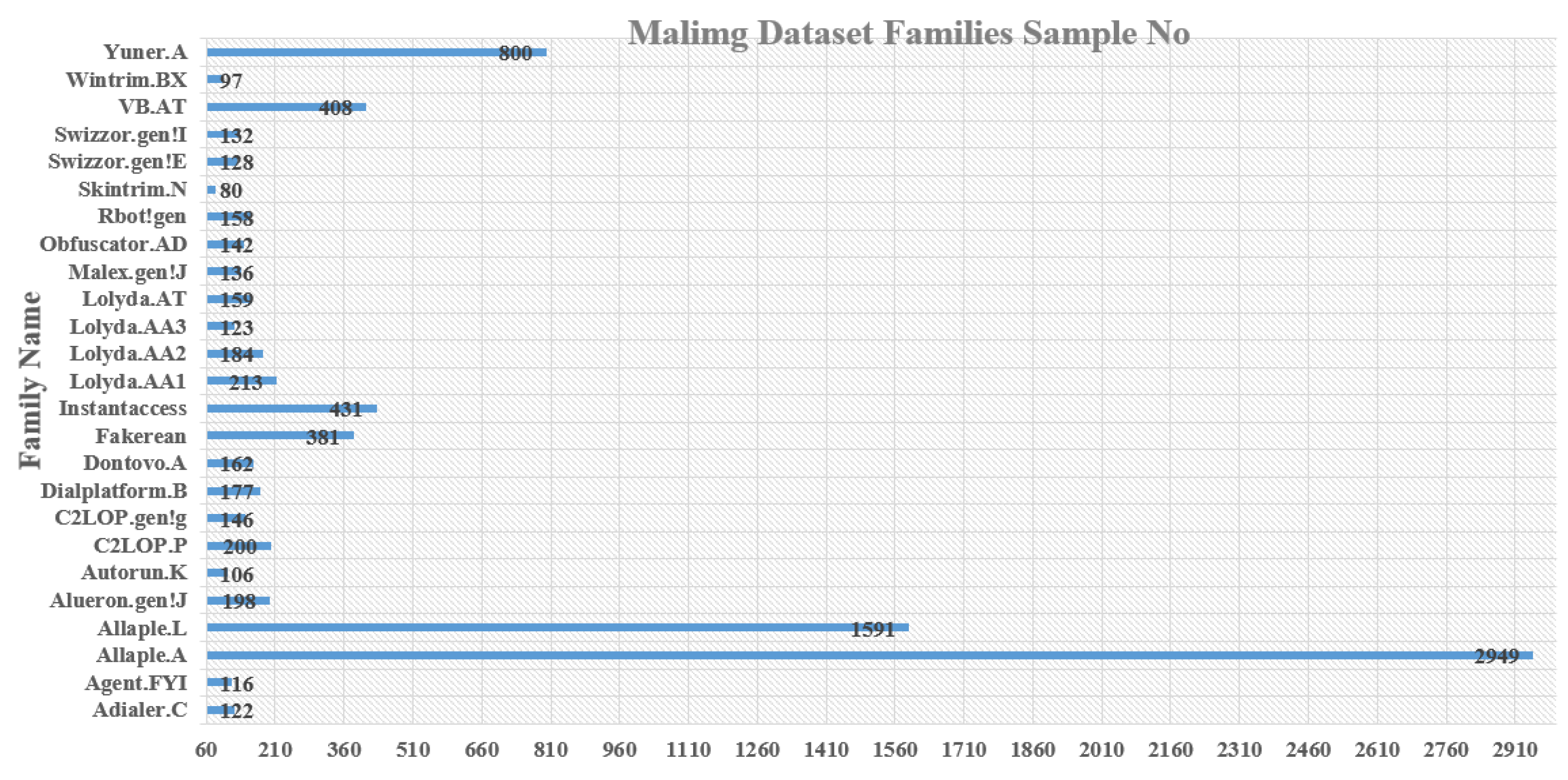
5.1. Datasets
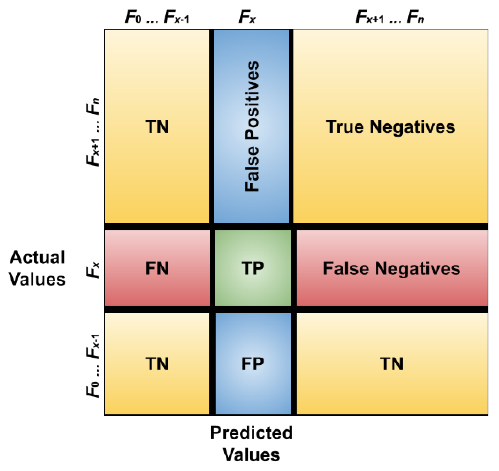
5.2. Performance Evaluation Metric
5.3. Evaluation Results
5.3.1. Performance Results of the Proposed Based on Tamura
5.3.2. Performance Results of the Proposed Based on GoogLeNet
5.4. Comparison with Alternative Methods
6. Conclusions
Author Contributions
Funding
Institutional Review Board Statement
Informed Consent Statement
Acknowledgments
Conflicts of Interest
References
- Berman, D.S.; Buczak, A.L.; Chavis, J.S.; Corbett, C.L. A survey of deep learning methods for cyber security. Information 2019, 10, 122. [Google Scholar] [CrossRef] [Green Version]
- Hemalatha, J.; Roseline, S.A.; Geetha, S.; Kadry, S.; Damaševičius, R. An efficient densenet-based deep learning model for malware detection. Entropy 2021, 23, 344. [Google Scholar] [CrossRef] [PubMed]
- Poudyal, S.; Akhtar, Z.; Dasgupta, D.; Gupta, K.D. Malware analytics: Review of data mining, machine learning and big data perspectives. In Proceedings of the 2019 IEEE Symposium Series on Computational Intelligence (SSCI), Xiamen, China, 6–9 December 2019; pp. 649–656. [Google Scholar]
- Nataraj, L.; Karthikeyan, S.; Jacob, G.; Manjunath, B.S. Malware images: Visualization and automatic classification. In Proceedings of the 8th International Symposium on Visualization for Cyber Security, Pittsburgh, PA, USA, 20 July 2011; pp. 1–7. [Google Scholar]
- Barath, N.N.; Ouboti, D.B.; Temesguen, M.K. Pattern recognition algorithms for malware classification. In Proceedings of the 2016 IEEE conference of aerospace and electronics, Dayton, OH, USA, 5–12 March 2016; pp. 338–342. [Google Scholar]
- Kosmidis, K.; Kalloniatis, C. Machine learning and images for malware detection and classification. In Proceedings of the 21st Pan-Hellenic Conference on Informatics, Larissa, Greece, 26–28 November 2017; pp. 1–6. [Google Scholar]
- Naeem, H.; Guo, B.; Naeem, M.R.; Vasan, D. Visual malware classification using local and global malicious pattern. J. Comput. 2019, 6, 73–83. [Google Scholar]
- Makandar, A.; Patrot, A. Malware class recognition using image processing techniques. In Proceedings of the 2017 International Conference on Data Management, Analytics and Innovation (ICDMAI), Pune, India, 24–26 February 2017; pp. 76–80. [Google Scholar]
- Verma, V.; Muttoo, S.K.; Singh, V.B. Multiclass malware classification via first-and second-order texture statistics. Comput. Secur. 2020, 97, 101895. [Google Scholar] [CrossRef]
- Sun, G.; Qian, Q. Deep learning and visualization for identifying malware families. IEEE Trans. Dependable Secur. Comput. 2018, 18, 283–295. [Google Scholar] [CrossRef]
- Gibert, D.; Mateu, C.; Planes, J.; Vicens, R. Using convolutional neural networks for classification of malware represented as images. J. Comput. Virol. Hacking Tech. 2019, 15, 15–28. [Google Scholar] [CrossRef] [Green Version]
- Agarap, A.F. Towards building an intelligent anti-malware system: A deep learning approach using support vector machine (SVM) for malware classification. arXiv 2017, arXiv:1801.00318. [Google Scholar]
- Çayir, A.; Ünal, U.; Daug, H. Random CapsNet forest model for imbalanced malware type classification task. Comput. Secur. 2021, 102, 102133. [Google Scholar] [CrossRef]
- Gibert, D. Convolutional Neural Networks for Malware Classification; University Rovira i Virgili: Tarragona, Spain, 2016. [Google Scholar]
- David, O.E.; Netanyahu, N.S. Deepsign: Deep learning for automatic malware signature generation and classification. In Proceedings of the 2015 International Joint Conference on Neural Networks (IJCNN), Killarney, Ireland, 12–17 July 2015; pp. 1–8. [Google Scholar]
- Nisa, M.; Shah, J.H.; Kanwal, S.; Raza, M.; Khan, M.A.; Damaševičius, R.; Blažauskas, T. Hybrid malware classification method using segmentation-based fractal texture analysis and deep convolution neural network features. Appl. Sci. 2020, 10, 4966. [Google Scholar] [CrossRef]
- Vasan, D.; Alazab, M.; Wassan, S.; Safaei, B.; Zheng, Q. Image-Based malware classification using ensemble of CNN architectures (IMCEC). Comput. Secur. 2020, 92, 101748. [Google Scholar] [CrossRef]
- El-Shafai, W.; Almomani, I.; AlKhayer, A. Visualized malware multi-classification framework using fine-tuned CNN-based transfer learning models. Appl. Sci. 2021, 11, 6446. [Google Scholar] [CrossRef]
- Khan, R.U.; Zhang, X.; Kumar, R. Analysis of ResNet and GoogleNet models for malware detection. J. Comput. Virol. Hacking Tech. 2019, 15, 29–37. [Google Scholar] [CrossRef]
- Bennasar, H.; Bendahmane, A.; Essaaidi, M. An overview of the state-of-the-art of cloud computing cyber-security. In Proceedings of the International Conference on Codes, Cryptology, and Information Security, Rabat, Morocco, 10–12 April 2017; pp. 56–67. [Google Scholar]
- Roseline, S.A.; Sasisri, A.D.; Geetha, S.; Balasubramanian, C. Towards efficient malware detection and classification using multilayered random forest ensemble technique. In Proceedings of the 2019 International Carnahan Conference on Security Technology (ICCST), Kota, Kinabalu, 1–3 October 2019; pp. 1–6. [Google Scholar]
- Ben Abdel Ouahab, I.; Bouhorma, M.; Boudhir, A.A.; El Aachak, L. Classification of grayscale malware images using the K-nearest neighbor algorithm. In Proceedings of the the Third International Conference on Smart City Applications, Karabuk, Turkey, 7–9 October 2019; pp. 1038–1050. [Google Scholar]
- Awan, M.J.; Masood, O.A.; Mohammed, M.A.; Yasin, A.; Zain, A.M.; Damaševičius, R.; Abdulkareem, K.H. Image-Based Malware Classification Using VGG19 Network and Spatial Convolutional Attention. Electronics 2021, 10, 2444. [Google Scholar] [CrossRef]
- Kumar, S.; Sudhakar. MCFT-CNN: Malware classification with fine-tune convolution neural networks using traditional and transfer learning in Internet of Things. Futur. Gener. Comput. Syst. 2021, 125, 334–351. [Google Scholar]
- Xiao, G.; Li, J.; Chen, Y.; Li, K. MalFCS: An effective malware classification framework with automated feature extraction based on deep convolutional neural networks. J. Parallel Distrib. Comput. 2020, 141, 49–58. [Google Scholar] [CrossRef]
- Simonyan, K.; Zisserman, A. Very deep convolutional networks for large-scale image recognition. arXiv 2014, arXiv:14091556. [Google Scholar]
- Szegedy, C.; Vanhoucke, V.; Ioffe, S.; Shlens, J.; Wojna, Z. Rethinking the inception architecture for computer vision. In Proceedings of the IEEE Conference on Computer Vision and Pattern Recognition, Las Vegas, NV, USA, 27–30 June 2016; pp. 2818–2826. [Google Scholar]
- Khan, S.H.; Sohail, A.; Khan, A.; Lee, Y.S. Classification and region analysis of COVID-19 infection using lung CT images and deep convolutional neural networks. arXiv 2020, arXiv:2009.08864. [Google Scholar]
- Glorot, X.; Bordes, A.; Bengio, Y. Deep sparse rectifier neural networks. In Proceedings of the Fourteenth International Conference on Artificial Intelligence and Statistics, Fort Lauderdale, FL, USA, 11–13 April 2011; pp. 315–323. [Google Scholar]
- Tanveer, M.; Shubham, K.; Aldhaifallah, M.; Ho, S.S. An efficient regularized K-nearest neighbor based weighted twin support vector regression. Knowl. Based Syst. 2016, 94, 70–87. [Google Scholar] [CrossRef]
- Bishop, C.M.; Nasrabadi, N.M. Pattern Recognition and Machine Learning; Springer: Berlin/Heidelberg, Germany, 2006; Volume 4. [Google Scholar]
- Ahmed, I.T.; Hammad, B.T.; Jamil, N. Image Copy-Move Forgery Detection Algorithms Based on Spatial Feature Domain. In Proceedings of the 2021 IEEE 17th International Colloquium on Signal Processing & Its Applications (CSPA), Langkawi, Malaysia, 5–6 March 2021; pp. 92–96. [Google Scholar]
- Huang, G.-B.; Zhu, Q.-Y.; Siew, C.-K. Extreme learning machine: A new learning scheme of feedforward neural networks. In Proceedings of the 2004 IEEE International Joint Conference on Neural Networks (IJCNN), Budapest, Hungary, 18–21 November 2004; Volume 2, pp. 985–990. [Google Scholar]
- Hoang, N.-D.; Bui, D.T. Slope stability evaluation using radial basis function neural network, least squares support vector machines, and extreme learning machine. In Handbook of Neural Computation; Elsevier: Amsterdam, The Netherlands, 2017; pp. 333–344. [Google Scholar]
- Jain, M.; Andreopoulos, W.; Stamp, M. CNN vs ELM for Image-Based Malware Classification. arXiv 2021, arXiv:2103.13820. [Google Scholar]
- Ahmed, I.T.; Hammad, B.T.; Jamil, N. A comparative analysis of image copy-move forgery detection algorithms based on hand and machine-crafted features. Indones. J. Electr. Eng. Comput. Sci. 2021, 22, 1177–1190. [Google Scholar] [CrossRef]
- Garcia, F.C.C.; Muga II, F.P. Random forest for malware classification. arXiv 2016, arXiv:1609.07770. [Google Scholar]
- Cui, Z.; Xue, F.; Cai, X.; Cao, Y.; Wang, G.; Chen, J. Detection of malicious code variants based on deep learning. IEEE Trans. Ind. Inform. 2018, 14, 3187–3196. [Google Scholar] [CrossRef]
- Goyal, M.; Kumar, R. AVMCT: API Calls Visualization based Malware Classification using Transfer Learning. J. Algebraic Stat. 2022, 17, 31–41. [Google Scholar]
- Wen, L.; Yu, H. An Android malware detection system based on machine learning. In Proceedings of the AIP Conference Proceedings, Tokyo, Japan, 1–2 November 2017; Volume 1864, p. 20136. [Google Scholar]
- Rezende, E.; Ruppert, G.; Carvalho, T.; Theophilo, A.; Ramos, F.; de Geus, P. Malicious software classification using VGG16 deep neural network’s bottleneck features. In Information Technology-New Generations; Springer: Berlin/Heidelberg, Germany, 2018; pp. 51–59. [Google Scholar]
- Choudhary, S.; Sharma, A. Malware detection & classification using machine learning. In Proceedings of the 2020 International Conference on Emerging Trends in Communication, Control and Computing (ICONC3), Sikar, India, 21–22 February 2020; pp. 1–4. [Google Scholar]
- Yeo, M.; Koo, Y.; Yoon, Y.; Hwang, T.; Ryu, J.; Song, J.; Park, C. Flow-based malware detection using convolutional neural network. In Proceedings of the 2018 International Conference on Information Networking (ICOIN), Chiang Mai, Thailand, 10–12 January 2018; pp. 910–913. [Google Scholar]
- Dahl, G.E.; Stokes, J.W.; Deng, L.; Yu, D. Large-scale malware classification using random projections and neural networks. In Proceedings of the 2013 IEEE International Conference on Acoustics, Speech and Signal Processing, Vancouver, UK, 26–31 May 2013; pp. 3422–3426. [Google Scholar]
- Hsien-De Huang, T.; Kao, H.-Y. R2-d2: Color-inspired convolutional neural network (cnn)-based android malware detections. In Proceedings of the 2018 IEEE International Conference on Big Data (Big Data), Seattle, WA, USA, 10–13 December 2018; pp. 2633–2642. [Google Scholar]


| Class ID | Family Name | Description | |
|---|---|---|---|
| Malware Kind | Sample No. | ||
| #1 | Adialer.C | Dialer | 122 |
| #2 | Agent.FYI | Backdoor | 116 |
| #3 | Allaple.A | Worm | 2949 |
| #4 | Allaple.L | Worm | 1591 |
| #5 | Alueron.gen!J | Trojan | 198 |
| #6 | Autorun.K | Worm | 106 |
| #7 | C2LOP.P | Trojan | 200 |
| #8 | C2LOP.gen!g | Trojan | 146 |
| #9 | Dialplatform.B | Dialer | 177 |
| #10 | Dontovo.A | Downloader | 162 |
| #11 | Fakerean | rogue | 381 |
| #12 | Instantaccess | Dialer | 431 |
| #13 | Lolyda.AA1 | PWS | 213 |
| #14 | Lolyda.AA2 | PWS | 184 |
| #15 | Lolyda.AA3 | PWS | 123 |
| #16 | Lolyda.AT | PWS | 159 |
| #17 | Malex.gen!J | Trojan | 136 |
| #18 | Obfuscator.AD | Downloader | 142 |
| #19 | Rbot!gen | Backdoor | 158 |
| #20 | Skintrim.N | Trojan | 80 |
| #21 | Swizzor.gen!E | Downloader | 128 |
| #22 | Swizzor.gen!I | Downloader | 132 |
| #23 | VB.AT | Worm | 408 |
| #24 | Wintrim.BX | Downloader | 97 |
| #25 | Yuner.A | Worm | 800 |
| Total | - | 9339 | |
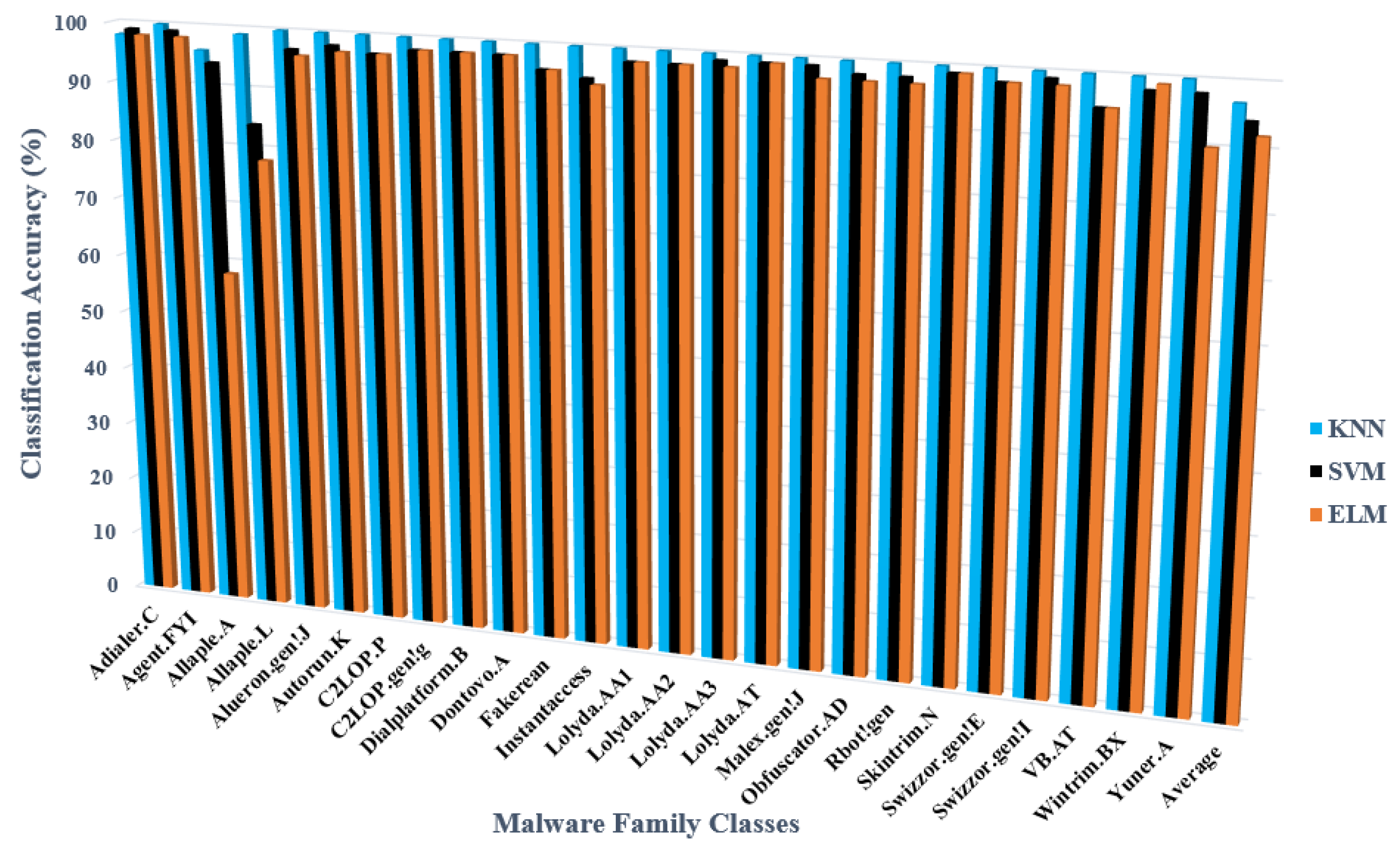
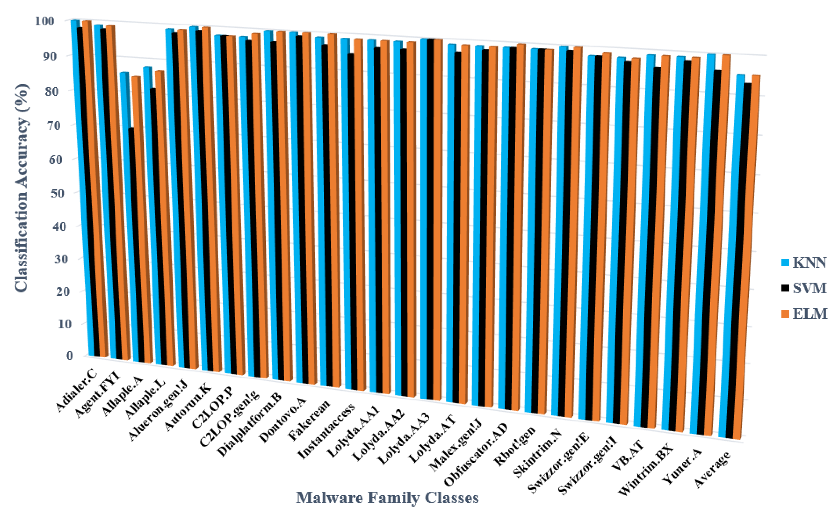
| Class ID | Family Name | Classification Accuracy (%) | ||
|---|---|---|---|---|
| KNN | SVM | ELM | ||
| #1 | Adialer.C | 100 | 98 | 100 |
| #2 | Agent.FYI | 99 | 98 | 99 |
| #3 | Allaple.A | 86 | 70 | 85 |
| #4 | Allaple.L | 88 | 82 | 87 |
| #5 | Alueron.gen!J | 99 | 98 | 99 |
| #6 | Autorun.K | 100 | 99 | 100 |
| #7 | C2LOP.P | 98 | 98 | 98 |
| #8 | C2LOP.gen!g | 98 | 97 | 99 |
| #9 | Dialplatform.B | 100 | 97 | 100 |
| #10 | Dontovo.A | 100 | 99 | 100 |
| #11 | Fakerean | 99 | 97 | 100 |
| #12 | Instantaccess | 99 | 95 | 99 |
| #13 | Lolyda.AA1 | 99 | 97 | 99 |
| #14 | Lolyda.AA2 | 99 | 97 | 99 |
| #15 | Lolyda.AA3 | 100 | 100 | 100 |
| #16 | Lolyda.AT | 99 | 97 | 99 |
| #17 | Malex.gen!J | 99 | 98 | 99 |
| #18 | Obfuscator.AD | 99 | 99 | 100 |
| #19 | Rbot!gen | 99 | 99 | 99 |
| #20 | Skintrim.N | 100 | 99 | 100 |
| #21 | Swizzor.gen!E | 98 | 98 | 98 |
| #22 | Swizzor.gen!I | 98 | 98 | 98 |
| #23 | VB.AT | 99 | 96 | 99 |
| #24 | Wintrim.BX | 99 | 98 | 99 |
| #25 | Yuner.A | 100 | 96 | 100 |
| Average | 95.34 | 93.23 | 95.42 | |
| Class ID | Family Name | Classification Accuracy (%) | ||
|---|---|---|---|---|
| KNN | SVM | ELM | ||
| #1 | Adialer.C | 98 | 99 | 98 |
| #2 | Agent.FYI | 100 | 99 | 98 |
| #3 | Allaple.A | 96 | 94 | 58 |
| #4 | Allaple.L | 99 | 84 | 78 |
| #5 | Alueron.gen!J | 100 | 97 | 96 |
| #6 | Autorun.K | 100 | 98 | 97 |
| #7 | C2LOP.P | 100 | 97 | 97 |
| #8 | C2LOP.gen!g | 100 | 98 | 98 |
| #9 | Dialplatform.B | 100 | 98 | 98 |
| #10 | Dontovo.A | 100 | 98 | 98 |
| #11 | Fakerean | 100 | 96 | 96 |
| #12 | Instantaccess | 100 | 95 | 94 |
| #13 | Lolyda.AA1 | 100 | 98 | 98 |
| #14 | Lolyda.AA2 | 100 | 98 | 98 |
| #15 | Lolyda.AA3 | 100 | 99 | 98 |
| #16 | Lolyda.AT | 100 | 99 | 99 |
| #17 | Malex.gen!J | 100 | 99 | 97 |
| #18 | Obfuscator.AD | 100 | 98 | 97 |
| #19 | Rbot!gen | 100 | 98 | 97 |
| #20 | Skintrim.N | 100 | 99 | 99 |
| #21 | Swizzor.gen!E | 100 | 98 | 98 |
| #22 | Swizzor.gen!I | 100 | 99 | 98 |
| #23 | VB.AT | 100 | 95 | 95 |
| #24 | Wintrim.BX | 100 | 98 | 99 |
| #25 | Yuner.A | 100 | 98 | 90 |
| Average | 96.84 | 94.24 | 92.07 | |
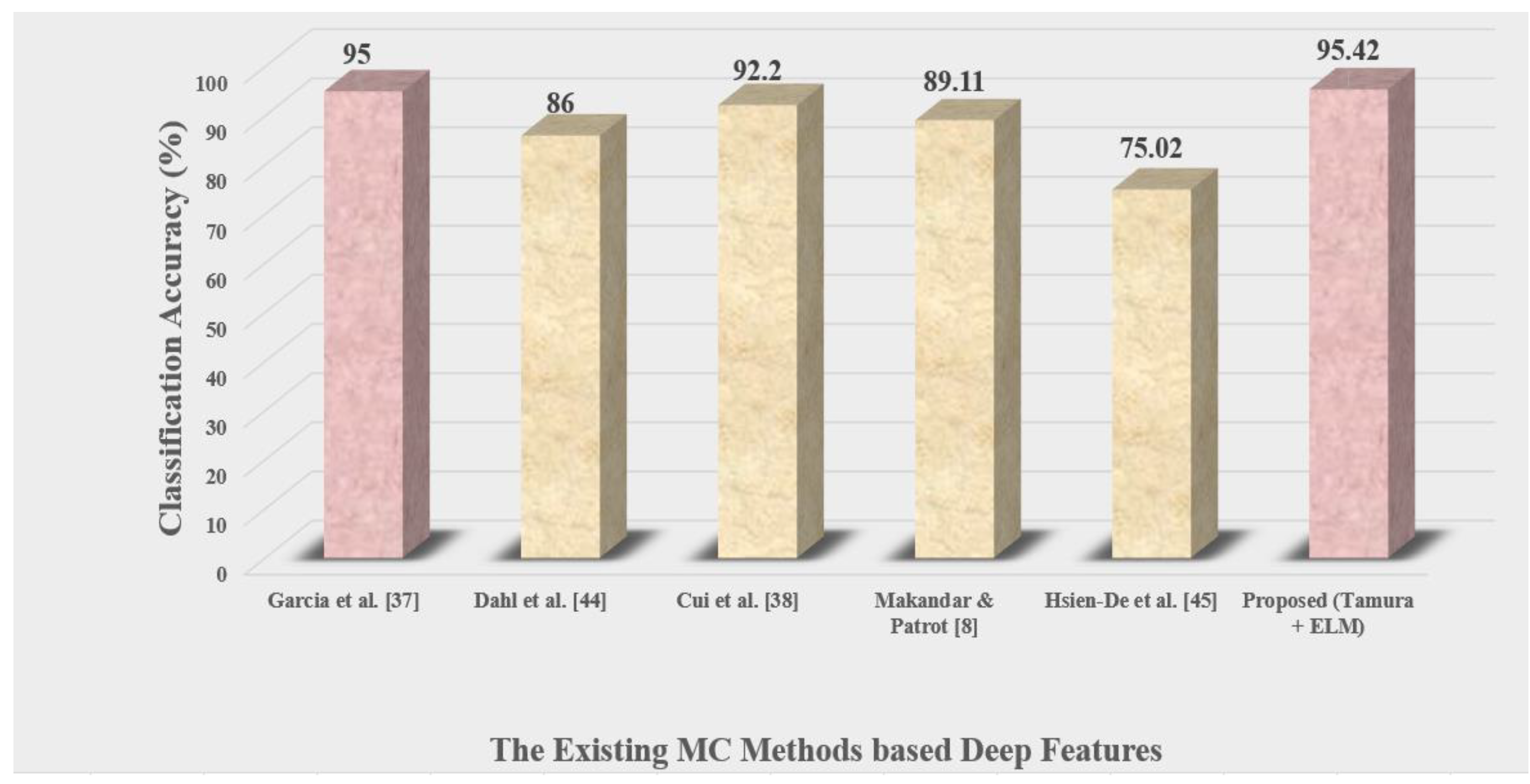
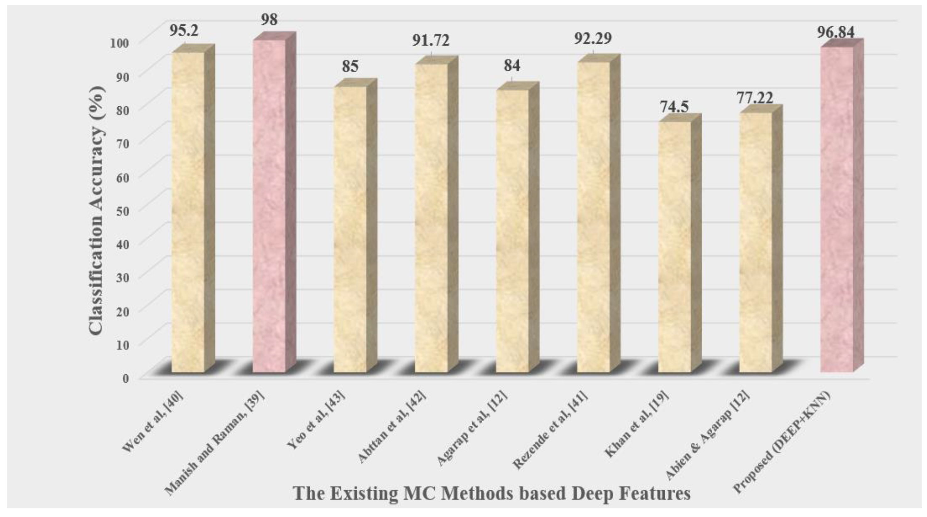
| Feature Method Domain | Methods | Feature Extraction | Classifier Kind | Dataset | Accuracy (%) |
|---|---|---|---|---|---|
| Handcrafted Features | Garcia et al. [37] | Texture features | Random Forest | Malimg | 95 |
| Dahl et al. [44] | Sparse binary features | Neural networks and logistic regression | Malimg | 86 | |
| Cui et al. [38] | GIST | SVM | Malimg | 92.20 | |
| Makandar & Patrot [8] | Gabor wavelet | KNN | Malimg | 89.11 | |
| Hsien-De et al. [45] | LBP | SVM | Malimg | 75.02 | |
| Proposed (Tamura + ELM) | Tamura | ELM | Malimg | 95.42 | |
| Deep Features | Wen et al. [40] | static and dynamitic analysis | SVM | Malimg | 95.2 |
| Manish and Raman, [39] | VGG-16, ResNet-50 and AlexNet | CNN | Malimg | 98.88 | |
| Yeo et al. [43] | CNN | MLP | Malimg | 85 | |
| Abttan et al. [42] | VGG16 | Naive Bayes | Malimg | 91.72 | |
| Agarap et al. [12] | CNN | SVM | Malimg | 84 | |
| Rezende et al. [41] | VGG16 | SVM | Malimg | 92.29 | |
| Khan et al. [19] | GoogleNet | GoogleNet | Malimg | 74.5 | |
| Abien & Agarap [12] | CNN | SVM | Malimg | 77.22 | |
| Proposed (DEEP + KNN) | GoogleNet | KNN | Malimg | 96.84 |
Publisher’s Note: MDPI stays neutral with regard to jurisdictional claims in published maps and institutional affiliations. |
© 2022 by the authors. Licensee MDPI, Basel, Switzerland. This article is an open access article distributed under the terms and conditions of the Creative Commons Attribution (CC BY) license (https://creativecommons.org/licenses/by/4.0/).
Share and Cite
Hammad, B.T.; Jamil, N.; Ahmed, I.T.; Zain, Z.M.; Basheer, S. Robust Malware Family Classification Using Effective Features and Classifiers. Appl. Sci. 2022, 12, 7877. https://doi.org/10.3390/app12157877
Hammad BT, Jamil N, Ahmed IT, Zain ZM, Basheer S. Robust Malware Family Classification Using Effective Features and Classifiers. Applied Sciences. 2022; 12(15):7877. https://doi.org/10.3390/app12157877
Chicago/Turabian StyleHammad, Baraa Tareq, Norziana Jamil, Ismail Taha Ahmed, Zuhaira Muhammad Zain, and Shakila Basheer. 2022. "Robust Malware Family Classification Using Effective Features and Classifiers" Applied Sciences 12, no. 15: 7877. https://doi.org/10.3390/app12157877
APA StyleHammad, B. T., Jamil, N., Ahmed, I. T., Zain, Z. M., & Basheer, S. (2022). Robust Malware Family Classification Using Effective Features and Classifiers. Applied Sciences, 12(15), 7877. https://doi.org/10.3390/app12157877