Article

A Hybrid Finite Element Method–Analytical Model for Classifying the Effects of Cracks on Gear Train Systems Using Artificial Neural Networks

by
Ronant de Paula Monteiro
1,*,
Amanda Lucatto Marra
2,
Renato Vidoni
1,
Claudio Garcia
2 and
Franco Concli
1
1
Faculty of Science and Technology, Free University of Bolzano-Bozen, Piazza Università 1, 39100 Bolzano, Italy
2
Department of Telecommunications and Control Engineering, Polytechnic School of the University of São Paulo, Avenida Professor Luciano Gualberto, Travessa do Politécnico 158, São Paulo 05508-900, Brazil
*
Author to whom correspondence should be addressed.
Appl. Sci. 2022, 12(15), 7814; https://doi.org/10.3390/app12157814
Submission received: 16 July 2022 / Revised: 29 July 2022 / Accepted: 31 July 2022 / Published: 4 August 2022

Abstract

:
Rotating machinery is fundamental in industry, gearboxes especially. However, failures may occur in their transmission components due to regular usage over long periods of time, even when operations are not intense. To avoid such failures, Structural Health Monitoring (SHM) techniques for damage prediction and in-advance detection can be applied. In this regard, correlations between measured signal variations and damage can be inspected using Artificial Intelligence (AI), which demands large numbers of data for training. Since obtaining signal samples of damaged components experimentally is currently unviable for complex systems due to destructive test costs, model-based numerical approaches are to be explored to solve this problem. To address this issue, this work applied an innovative hybrid Finite Element Method (FEM)–analytical approach, reducing computational effort and increasing performance with respect to traditional FEM. With this methodology, a system can be simulated with accuracy and without geometrical simplifications for healthy and damaged cases. Indeed, considering different positions and dimensions of damages (e.g., cracks) on the tooth roots of gears can offer new ways of damage investigation. As a reference to validate healthy systems and damage cases in terms of eigenfrequencies, a back-to-back test rig was used. Numerical simulations were performed for different cases, resulting in vibrational spectra for systems with no damage, with damage, and with damage of different intensities. The vibration spectra were used as data to train an Artificial Neural Network (ANN) to predict the machine state by Condition Monitoring (CM) and Fault Diagnosis (FD). For predicting the health and the intensity of damage to a system, classification and multi-class classification methods were implemented, respectively. Both sets of classification results presented good prediction agreement.

1. Introduction

Rotating machines are widely used in industry and gearboxes are extensively employed in this regard since they have high efficiencies and compact structures. However, due to constant operation and possibly intense working conditions, damage to such systems may occur [1]. These damages, also known as failures of mechanical systems, can cause recognizable characteristics in vibrational signals, which can be used for early fault diagnosis (FD) [2]. In this regard, condition monitoring (CM), where condition parameters (e.g., vibrations) in machinery are monitored to identify indicators of changes that might result in damage, can be essential for FD. Indeed, CM can be used for decision making in the planning of predictive maintenance to prevent catastrophic problems. Thus, CM can be a potential approach to decrease downtimes in production systems [3]. An accurate CM indicator is the key factor in FD and in the prediction of the remaining useful life of the components of a system [4]. Not only does it increase economic efficiency [5], it can also increase safety for humans and machines [6]. The detection of a change in the vibration indicators of a rotor system can be approached by employing signal processing methods, which are required to highlight information characteristics prior to load identification [7]. The current state of the art related to the analysis of vibration signals for FD foresees the periodic monitoring of these processed signals and the comparison of them over time. The monitoring of vibration spectra, specifically, can be considered a pattern recognition task. This is historically a primary application of Artificial Intelligence (AI) techniques such as Artificial Neural Networks (ANN) [8]. Thus, by using AI methods, emphasis can be given to the fact that when vibrations are used to extract features for FD, the correlation between the measured signal and the current status of the structure of the machine is very important [9].

1.1. Failure of Mechanical Systems

Fracture mechanics is mainly the study of the complex stress field around the tip of a crack, which is generally used to investigate whether an existing crack will propagate in a system. Additionally, fatigue analysis is the study of fracture behavior under repeated cyclic loading. When the material of a structure gets worn out due to repetitive loads, fatigue occurs, which may result in failure [10]. Thus, gearboxes and their components, such as gears, shafts, bearings, rotors, couplings, and housings, can be subject to many types of failures, which can influence the systems and affect their behavior and working operations. Furthermore, even though several gearbox components are subject to failures, most of the damages occur in the gears. Considering the failure modes of mechanical systems, cracking, pitting, scuffing, wear, and spalling are generally considered the common ones [11]. In this regard, a number of referenced scholars have conducted research into the failure of mechanical systems. Among others, ref. [12] developed research for investigating the consequences of mild wear and rolling–sliding with respect to contact fatigue of gears. Ref. [13] used dynamic modeling to study a planetary gearbox analyzing the effect of clearance with respect to damage to its components. A numerical model was created in [14] to study a wind turbine gear and check the behavior of contact fatigue to analyze its responses. Ref. [15] investigated the effects of a crack on the gear mesh stiffness of a gear by adopting an analytical approach and then applied a dynamic model for understanding the behavior of a planetary gear.
The detection (diagnosis) of failure can be understood as the identification of a specific condition (damage) of a machine based on the presence of symptoms. Diagnosis can isolate a symptom of a gearbox, whose characteristics such as the design, degradation process of certain faults, production technology and change in condition can provide important information for further decision making related to the detection of failure [16]. Then, the failure mode requires a good understanding of each possible case of damage, so that techniques for evaluating their indicators can be developed. For this, a great number of faults can be detected by physical examination of a system component. Such examinations can be performed using various techniques, such as X-ray, microscopic, magnetic rubber methods, etc. However, it is difficult to apply such techniques without removing the relevant component from the mechanical system and, in specific cases, without damaging the component. In addition, some inspections for verifying a system require human operators to visually inspect the structure. Thus, the number of components fabricated, the variety of damaged structures, and inspection time, for instance, make this procedure unfeasible [17]. In this case, for periodic monitoring, other effective fault-detection techniques should be used in place of intrusive damage detection. In addition, monitoring techniques are considered suitable ways to inspect the evolution and level of a damage in a structure [18]. The methods used for diagnosing gearbox problems are based on vibration analysis, the spectra for which can be collected from, e.g., the housing of the gearbox. Vibration analysis is usually carried out to detect the presence and location of damage as well as to discover its pattern and harshness level. During operation, housing vibrations can indicate gearbox faults by comparing signals with a baseline over a period of time [19]. Indeed, this diagnostic can reveal information related to the fault stage and provide evidence for its evolution; thus, the estimation of the machine’s residual life can be properly analyzed for maintenance action.

1.2. Vibration Analysis

Vibration analysis can be considered a fundamental approach in respect of CM [20]. It has been extensively used over the past years and it is considered the most common process for CM, which is broadly applied in this field. Since vibrations can be found in all rotating machines, a modification or damage to any system component can modify a vibrational signature. Most of the kinds of damage that a rotating machine is subject to have vibration patterns which can be specified in relation to the structure, development, construction, and health state of the machine components. All machines that have moving components can substantially generate sound and vibration from specific characteristics, and these characteristics can change according to their behavioral process if the machine condition changes. Indeed, such change can allow early damage detection before the occurrence of a severe problem [21]. Moreover, vibration analysis is able to detect abnormal vibration events which can enable an evaluation of the overall condition of the object and the identification of variations in its spectra. Then, CM can be used as a pattern recognition process to compare spectra over time and identify these variations. Since vibration analysis is a process that monitors the levels and patterns of vibration signals within a structure, excessive vibration in a machine (e.g., gearbox transmission system) can indicate damage. Indeed, by analyzing spectra, it is possible to identify the frequencies and relate the differences to the baseline (signature) with the mechanical characteristics of the transmission system and thus identify potential defects. With respect to this issue, previous works have reported that the frequencies of a system can shift given the occurrence of damage. Ref. [22] observed differences in the amplitudes of gear harmonics which gave indications of gear faults. Ref. [23] showed that a noise-like distortion in the vibrational response of a structure, for SHM, can be nonstationary and thus requires a time–frequency analysis. Ref. [24] analyzed the relationships among the natural frequencies of the system studied and compared the least affected to the most affected modes of vibration, allowing the method to be more sensitive to damage. Ref. [25] used an SHM methodology to predict the edge frequencies of a wind turbine blade to check the health state of the system. The proposed methodology was able to identify when the blades started behaving differently over time. Ref. [26] researched a frequency band identification framework for gearbox fault diagnosis under time-varying operating conditions. Ref. [27] studied a technique for cases in which the monitoring of vibrations excited by machine operations with accelerometers is required. According to this technique, mechanical coupling between sensors and measurement objects influences high-frequency vibrational responses. In addition, excessive vibration can reflect the characteristics of the damage problem, which is generally related to the ratio of the forces that can act on the gear. Indeed, time-varying mesh stiffness and related errors can affect the dynamic variations of meshing forces [28].
The procedures used for gear vibration analysis can be subdivided into three categories: time domain, frequency domain, and time–frequency domain. Time domain procedures use tools to determine the condition of a rotating machine and methods to collect and interpret data to investigate patterns and trends in terms of time. Frequency domain refers to an analytic environment wherein signals are displayed in terms of frequency. The time–frequency domain covers two techniques, whose investigation comprehends the study of signals in both time and frequency domains. Moreover, the harmonics are considered important characteristics to be analyzed with respect to amplitude and range of frequency. In addition, analysis of the modulation phenomena associated with sidebands may indicate a fault condition in the system depending on the amplitude of the spectra. Generally, this analysis is related to vibration signals, which are sources of damage identification and detection information. Indeed, sidebands can be used to associate these sources with the characteristics of rotating components [29]. Some factors that decisively affect the indication of a fault and its characteristics are related to the level of vibration, rotational speed of the components of the system, background noise, transducer location, load-sharing characteristics and dynamic influences between components in contact. The foregoing descriptions articulate the basic principle of many CM methods. Thus, by advancing vibration analysis, the AI approach is recommended for the CM field due to its effectiveness in developing fault diagnosis techniques for mechanical systems [30].

1.3. Artificial Intelligence (AI)

AI deals with problems that need intuition to be solved, such as pattern recognition and prediction. The process of defining a problem, determining its cause, and then finding alternatives and solutions is called problem-solving, which is a technique very often used to solve problems in AI. Another example of a technique used in this context is learning, which in AI can be recognized as the way the machine acquires the necessary information to achieve its goal to recognize and predict what is needed, in an accurate way. Machine Learning (ML) methods, which are part of the AI field, rely on large numbers of data. Then, model parameters need to be tried and adjusted many times to find the optimal settings for a gearbox analysis [31], which is the system considered in this work. Hence, ANN and Deep Learning (DL) methods, among other technologies and algorithms that are also part of the AI field, can be explored.
Considering these methodologies, one technique that can be used to approach the problem of FD in rotating machines is the ANN. The ANN is a numerical methodology composed of several processing elements that are digitally interconnected. These processing elements, called neurons, are considered simple; however, they can efficiently process information by their dynamic state responses to external inputs [32]. On the other hand, several layers of interconnected neurons are used by DL to extract patterns that can repeat, in a predictable manner, important aspects of raw data. Thus, FD approaches, in the current context, are being widely implemented with the development of ML and DL methodologies [33], which have the potential for further growth.
AI is considered one of the most affordable approaches for FD and CM analysis due to its automated and efficient status. Indeed, it is one of the preferred techniques in the industry [34], because the state of the machine (healthy or damaged) can be recognized automatically. ANN, which is a classical approach used in ML, can be applied to FD in machines in three stages. First, in data collection, data are regularly collected through sensors that are mounted on specific structures of machines. Feature extraction—the second stage—divides into two sub-stages: the first applies time, frequency, or time–frequency domain techniques to extract features from collected data, which characterize the health state of the machine; the second sub-stage selects data and their attributes that can be used for the detection of the health state of the machine, which can be achieved through an exploratory analysis of the database. Here, the data are categorized by defining the objects (e.g., the ranges of the frequencies and amplitudes) that can be properly used in the next phase. In the third stage—health state recognition—FD-based models are created by establishing a relation between the characteristics of the data extracted and the health state of the machine [35]. This is accomplished by training an ANN with the categorized data. In this way, the ANN turns into a model that is able to recognize the state of the machine by creating a relation between the input samples without labels, due to the training task initially performed, and a variety of these samples with labels.
Therefore, several researchers have used ML to study different ways of monitoring the health states of systems and/or diagnosing faults in rotating machines. In this regard, four different detection methods for epicyclic gearbox health monitoring were implemented and tested in [36]. The authors implemented methods such as nearest-neighbor distance-based, data distribution, and two model-based methods involving ANN. An automated FD was introduced in [37] to classify faults in gears using ANN. An ANN-based approach was used in [38] for gear CM, whose principal component analysis approach showed effectiveness in its results. A wind turbine planetary gearbox was used in [39] to develop an application of ANN for FD. An FD model for gears was developed by [40] using ANN techniques to give an effective diagnosis of faults. A precise and efficient FD method was created in [41] using a deep learning framework for rotating machinery. A method for FD in the pitting of gears was developed in [42] using raw vibration signal data. ANN can thus be seen as a technique that is widely used to diagnose damage to systems due to its effectiveness in the context of monitoring machine states. Additionally, the acquisition of failure datasets is difficult due to the high number of samples required for training an ANN, which can make this approach impossible [2]. Numerical analysis is one of the procedures that can be used to acquire and process data (objects) for the creation of datasets appropriate to train ANNs, given the need for databases with consistent data to obtain better output responses from algorithms when implementing ANN architectures.

1.4. Motivations of This Research

The intense working conditions of a gearbox can cause recognizable characteristics in vibration spectra when specific system components are monitored. However, this approach usually does not operate in real time, occasioning a delay in maintenance actions such that opportunities to make timely interventions and address developing faults may be missed. Thus, SHM has the advantage of maintaining a system under constant control with the assistance of an online monitoring. CM techniques can be used to check and repair a system synchronously instead of only checking it at fixed intervals. This can avoid downtimes, which can be due to failures, as well as guarantee the working life of a machine [43] and even its prolongation via structural modification approaches [44,45]. Moreover, this efficient procedure benefits its operation in terms of low maintenance actions and economic efforts since it has the capability of inspecting the system continuously.
To implement such a technique, an experimentally based configuration, which provides a realistic view of the process, can be inviable due to the huge costs involved, especially when it comes to the experimental replication of damage to a system. Hence, a model-based approach can be a solution; the data responses of models can be used preliminarily for SHM, and the data generated from analytical and numerical models can be employed for modeling and training. Indeed, for numerical simulation, less time and equipment are required to obtain a large number of experimental data from a complex structure, especially for systems for which it is a complicated matter to develop tests for carrying out experimental investigation [46]. Considering these conditions, in this study, an innovative hybrid FEM–analytical model for a test rig system was implemented to reduce the computational effort and increase the numerical performance compared to a traditional FEM approach. With this model, complex systems can be numerically simulated with good accuracy and without geometrical simplifications. Healthy and damaged (e.g., crack) conditions can be evaluated, considering that the approach can generate vibrational results in terms of spectra for both sorts of conditions. In addition, adding different positions and dimensions to the cracks on the tooth roots of gears, as well as adding multiple damages separately or simultaneously to them, can offer new ways to investigate the health states of systems.
After performing the numerical simulations, the displacements from each simulated condition could be extracted and a damage identification could be made based on ML algorithms using a database of simulated signals in healthy and faulty conditions. Moreover, in the present paper, the detection of damage to the test rig system was performed using the ANN approach, adopting the following three procedures: (1) information extraction of signals, which can be shown in time and frequency domains; (2) characterization of extractions, that is, the transformation of the coarse data into applicable data which generate aspects that preserve numerical information in its original form; and (3) classification, which is used for feature categorization. Then, the method of classification parameters used to detect and predict damages and their severity conditions could be applied. In this way, a framework is established to diagnose the state of the system (classification technique) and multiple classes of gearbox faults (multi-class classification technique). Therefore, these outcomes are a set of visualized decision rules of the damage characterization framework that can be automated through machine learning algorithms, thus presenting a starting point for the implementation of effective prognostic algorithms for predictive maintenance. Predicting damage to a system and defining its severity are considered the goals for this work, which can be achieved by the support of the ANN approach.
The structure of this research paper is as follows. The characteristics of the test rig are presented in Section 2. The numerical approach is then presented in Section 3, with a focus on the application scenario together with details of the hybrid model in both healthy and damaged conditions. Section 4 presents the ANN approach and its analyzed features. The results of damage identification algorithms for detection and severity classifications are provided in Section 5, while the discussion of results is presented in Section 6. Then, Section 7 completes the paper.

2. Gearbox Characteristics

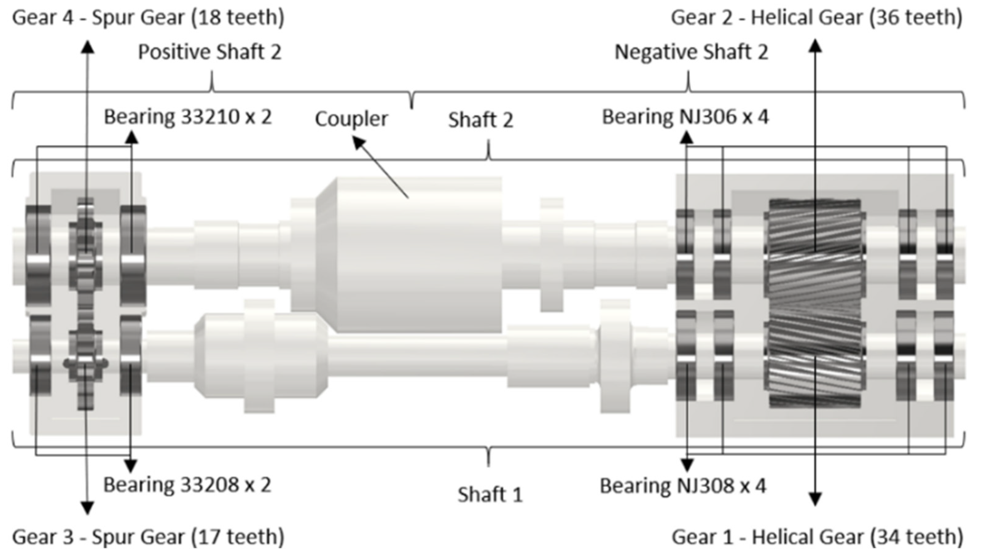
The test bench (test rig system) used for this work is depicted in Figure 1. The system is located at the Polytechnic University of Milan and is composed of 2 shafts, 12 bearings, and 2 gearboxes (service and test) forming 2 gear pairs (Figure 2). Each gear pair has the same center distance and the same gear ratio, and they are connected by two parallel shafts (shafts 1 and 2), obtaining a mechanically closed circuit. Shaft 2 is composed of a rotating servo-hydraulic torque actuator (coupler) that decouples the two semi-shafts (positive shaft 2 and negative shaft 2). The torque is applied to the system by traditional mechanical coupling, which procedure can be similar to the one performed in a FZG (Forschungsstelle fur Zahnrader und Getriebebau) test rig, the technical institute responsible for which develops studies about gears and drive mechanisms. In this study, the system was substituted by a hydraulic actuator of shaft 2. Since this can be used in different operations and varying modes, the applied torque can be changed to test the required system in different modes, which enables a test with variable load. The torque through shaft 1 can be measured by strain gauges, and the vibration signals can be collected through the housing (the location used for the analysis of this paper) by piezoelectric accelerometers. This mechanism, arranged in a closed mechanical loop, applies a rotation to the two semi-shafts to induce equal and opposite torques in the tested gears, and this configuration can be used to test gearing at varying speeds. The test bench is controlled by an inverter, and it is driven by an asynchronous induction motor, which is electric. As a result, the system needs to supply the energy losses, which requires a system equipped with two independent lubrication circuits. The first refers to the hydraulic actuator and the service gearbox, while the second refers to the test gearbox, in which properties such as lubrication and temperature can be adjusted. Therefore, the maximum torque, speed, and lubrication for this test bench are 1000 Nm, 3000 rpm, and 120 °C, respectively [47].
The spur gears, components of the test gearbox, were used to investigate cases of damage. In this study, they were used for evaluating the consequences of cracks in the system. The main parameters of the test bench, including information about the test gears, are presented in Table 1.
Studies of this type of machine can be used for research related to predictive maintenance of industrial rotating machinery. In addition, ML techniques can be used for FD by performing vibration analysis of a system and this approach can prevent the machine from operating in periods in which the components of the system are degrading [48]. Thus, it is important to consider these essential gear train parameters in order to investigate the dynamic behavior of a system and properly implement the ANN architecture to predict different types and levels of damages for each system.

3. Modeling, Implementation, and Numerical Simulation

A test rig dynamic analysis was performed using Transmission3D (T3D) software [49], the aim of which was the extraction of displacements to further analyze vibrations and their spectra to predict damage. The test rig can be configured in different regimes that can be applied to the system. The traditional FEM describes the macroscopic deflection of components, while T3D solves analytically the contact between bodies. Generally, a mesh refinement, to provide convergence and properly simulate a contact, is required in the traditional approach. Moreover, in order to generate good numerical results and obtain converged simulations, the flanks in the region of the gear teeth, where the main analysis take place, must be discretized with a very fine mesh. This is usually performed due to the contact position of the gears and the variation of their engaged surfaces during operation, which increases the number of equations to be solved [50]. Thus, this problem can be solved in the T3D environment. As an example, in the approach applied by [51], the FEM was used as the second stage of product development. It was performed due to the fact that lumped parameters (e.g., stiffness of gearbox components) were determined to support the analysis of the analytical model. This type of numerical simulation, which is a highly effective technique for this type of problem, provides an accurate inspection of the mesh stiffness model. In this way, several engagement positions need to be simulated to perform a consistent analysis related to the contact of the gears and acquire a mean value related to them. This is due to the variation in the stiffness during the engagement of the gears. For accurate results, a mesh sensitivity analysis should also be performed for the contact regions so that the elements and nodes in these areas can activate a simulation that converges properly. Subsequently, the complexity of creating feasible finite element (FE) models of geared systems, including the test rig presented in this research, and the expansion time of their simulations make the traditional FEM approach unfeasible in some cases. Moreover, even being completely useful for some systems, it can be replaced by a more efficient one. Thus, each contact during the engagement was analytically solved in this method through a few equations, without using a robust mesh refinement. This benefits the entire process objective through a hybrid FEM–analytical approach and effectively reduces the time of each simulation.
The simulation of transmission systems, in which characteristics can be complex and widely extensive in geometrical matters, is performed through an approach specifically developed for this, a hybrid FEM–analytical approach. All the internal components of the system (e.g., gears, shafts, and bearings) are modeled entire; thus, accuracy with respect to system response can be achieved. Since the deformations originated by contacts between rotating machine components were approached based on the Hertzian theory, the method used in this research paper adopts a solution different from traditional FE, which refers to the macroscopic deflection of the components under analysis. Given this, the constant contacts of the rotating components under analysis, such as gear teeth and internal bearings, need mesh refinement. This is due to the fact that a FE simulation of this magnitude needs to guarantee convergence so that the software can correctly simulate the desired system. Furthermore, mesh refinement is also required when the contacts and couplings of the variable rotating components are analyzed in order to obtain convergence with the simulated system. On the other hand, the model presented in this research paper solves, for each contact of the acting components, an additional equation through a relatively coarse grid [52]. This makes the computational effort relatively low, as the number of equations which need to be solved is reduced. Therefore, this process is carried out without changing important FE features, such as accuracy and simplification of the system. In fact, the distance between the points located on the contacting surfaces of the bodies under analysis is small. In this way, they can be activated before the load is applied to the system [53]. Then, the normal surfaces can be identified and the regions where the contacts are performed can be estimated by Hertzian equations. Indeed, the Hertzian contact grid is overcome by a larger computational grid, which is arranged around each contact under analysis. This, in turn, can be projected onto both the surfaces in this solver stage and the contact pressures that are computed through this procedure, which are not sensitive to grid size. Therefore, additional details are given in [52].
To approach this problem, the following mathematical statement can be expressed. First, the displacement, u ( r i j ; r ) , of point r is evaluated. Due to the application of a load at the surface grid point, r i j , the following Equation (1) is expressed:
u ( r i j ; r ) = [ u ( r i j ; r ) u ( r i j ; q ) ] + u ( r i j ; q ) ,
where the first term, [ u ( r i j ; r ) u ( r i j ; q ) ] , can be evaluated by applying the surface integral technique. The second term, u ( r i j ; q ) , can be acquired from the FE model. Then, q can be described as a point inside the solid body. Its distance is considered far from the surface.
Instead of using the FE responses, the estimation of the term between square brackets, which can be more affordable using the Boussinesq half-space solution, represents the deflection of r with respect to point q [54]. In fact, the term will not be affected by the deformation of the body; however, the last term, u ( r i j ; q ) , is not substantially affected by stresses of the local surfaces. In this way, if q is located in a region distant from the surface, the term u ( r i j ; q ) can be better estimated by the model of the solid body by using FEM.
Therefore, the q location is known as the “matching” point. Thus, in order to approach this problem, by combining the FE surface integral and FEM, a group of points can be used instead of a single point q [55]. Supplementary details can be found in [56].

3.1. Numerical Simulation

The model setup (Figure 3), for healthy and damaged cases, considers a speed of 3000 rpm, a torque of 1 N, and 6000 steps. To address a feasible number of steps for each simulation, the following observation was considered: the greater the number of steps, the more the time to simulate the desirable system.
Then, some assumptions and investigations regarding aspects of the spectrum and the number of steps were also performed for the system presented in this paper. First, the computational capacity for simulating each system was considered so that the work would be performed in an appropriate time. Second, at least four periods of rotation were desired in order to achieve a proper visualization of spectra and their characteristics in the time domain. Third, delimitation of the range of the data acquired from each FEM simulation was accomplished in order to obtain a suitable sampling (discretization) time. Then, each system simulation generated data with reference frame deflection in the z-direction. Fourth, the data were used to post-process a clean signal in the time and frequency domains, considering the visualization of the harmonics, sidebands, and gear mesh frequencies (GMFs). The latter defines the resolution of the analysis, which is very important for accurate results and the determination of sampling time. The calculation of the GMFs of the two gear pairs (test and service gearboxes) can be expressed as:
G M F = Z m i n   ·   n m i n 2 π ,
where z is the number of teeth and n is the rotational speed. Finally, the last investigation was related to the delimitation of the range of the frequencies to be used in the ANN application to avoid overfitting.
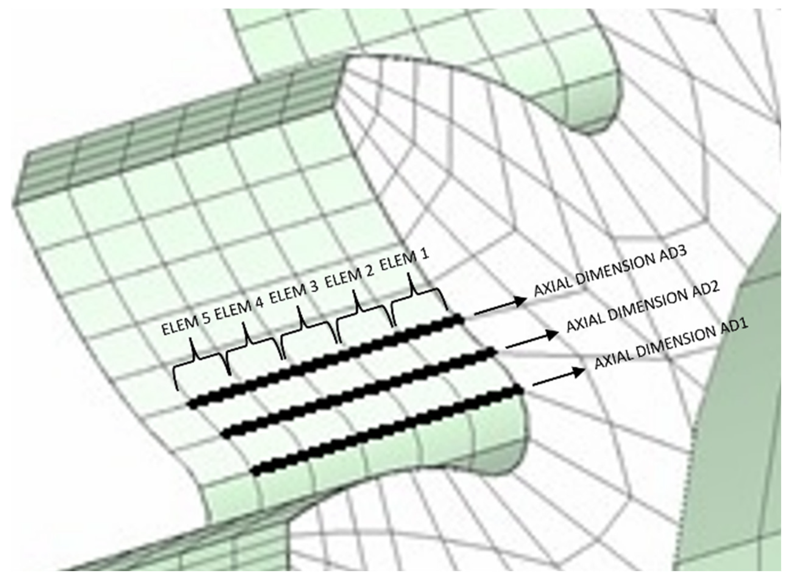
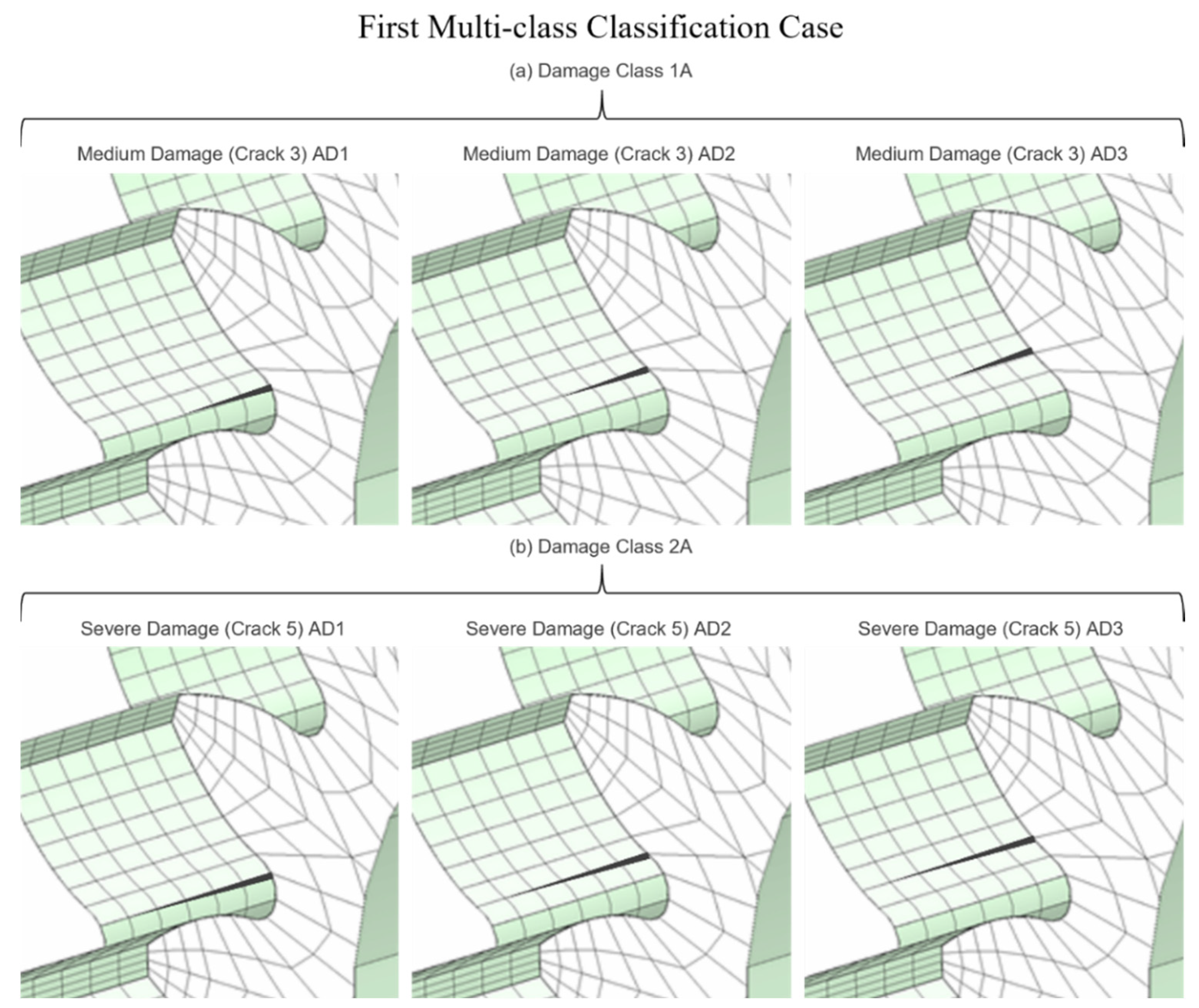
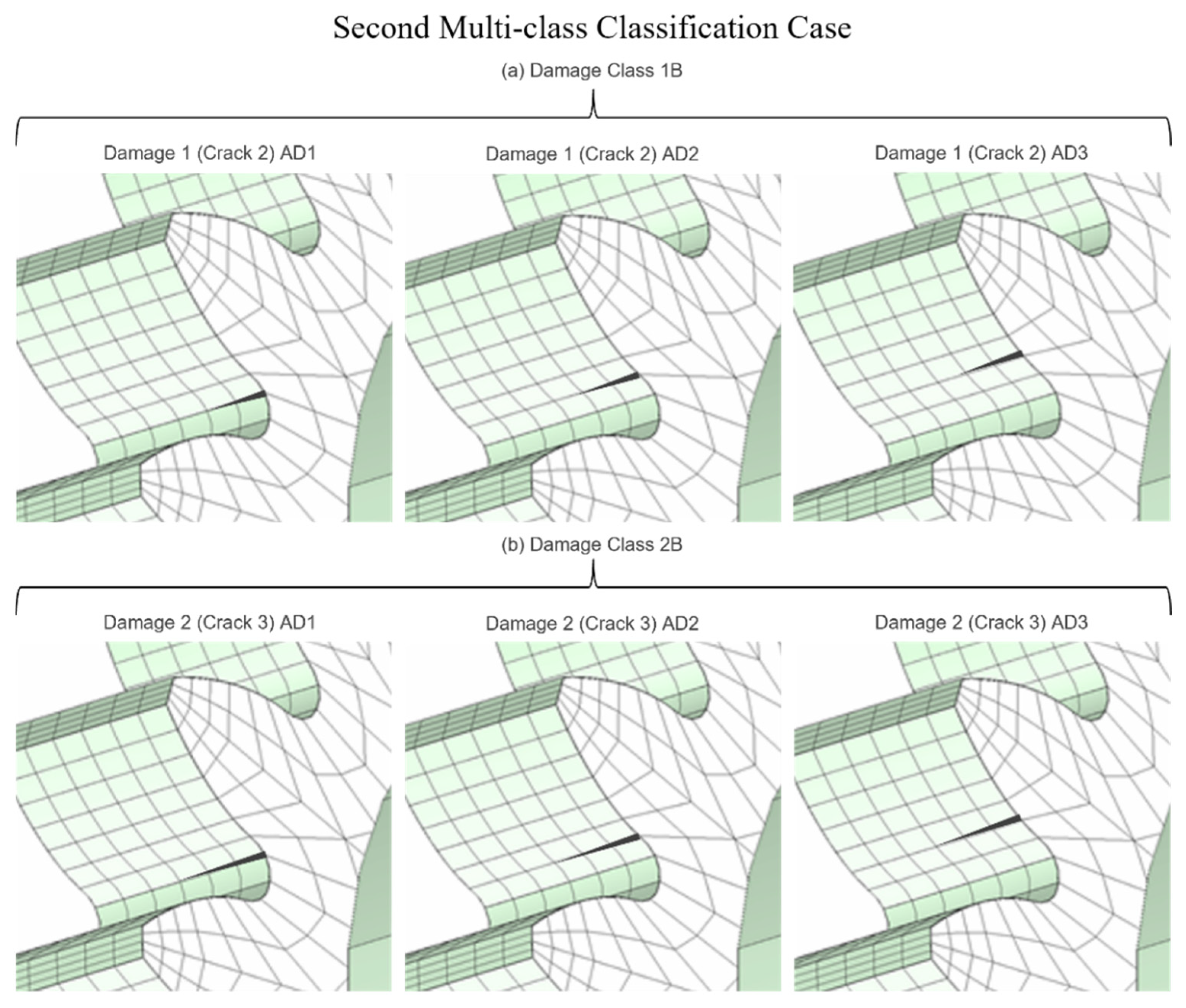
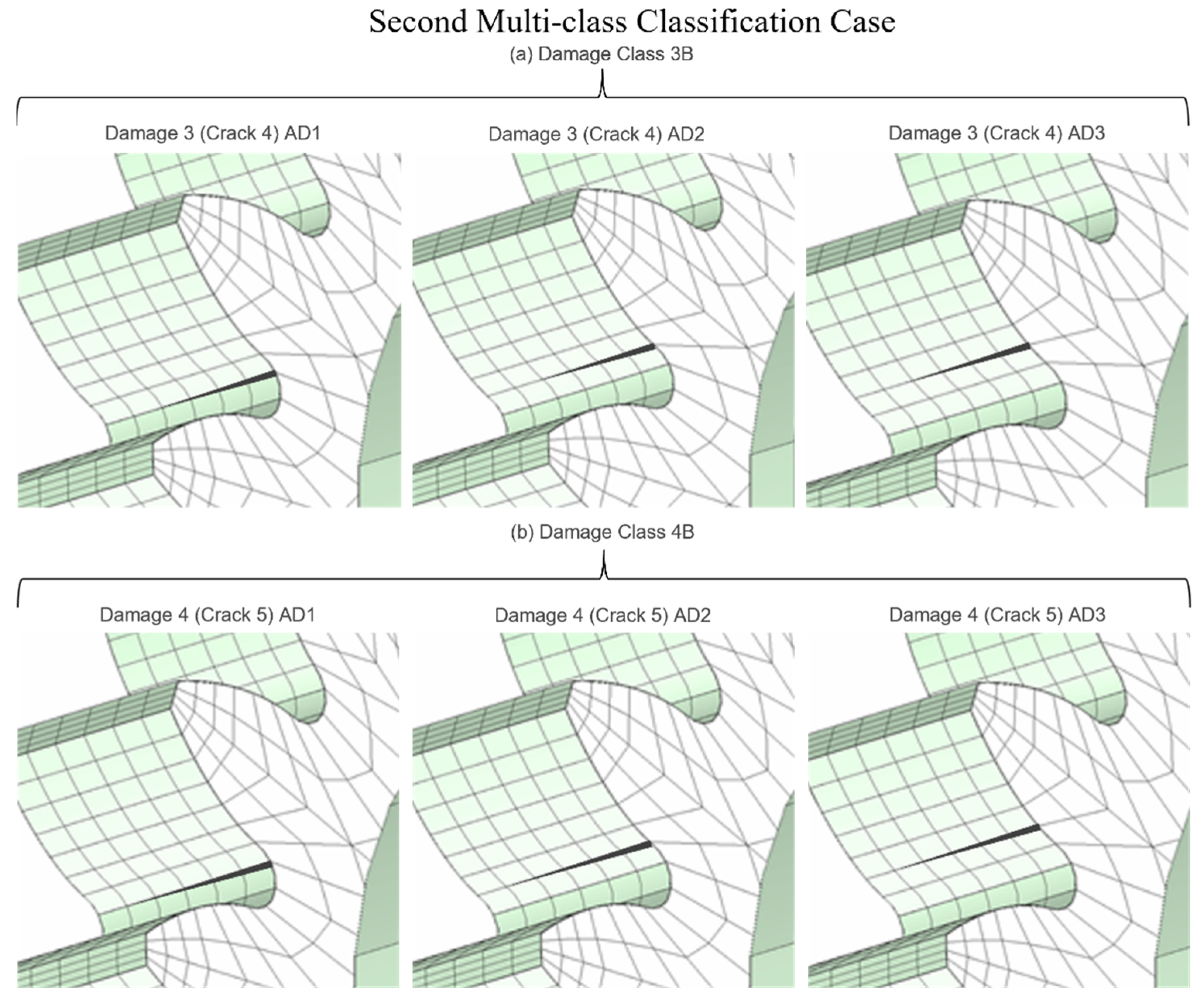
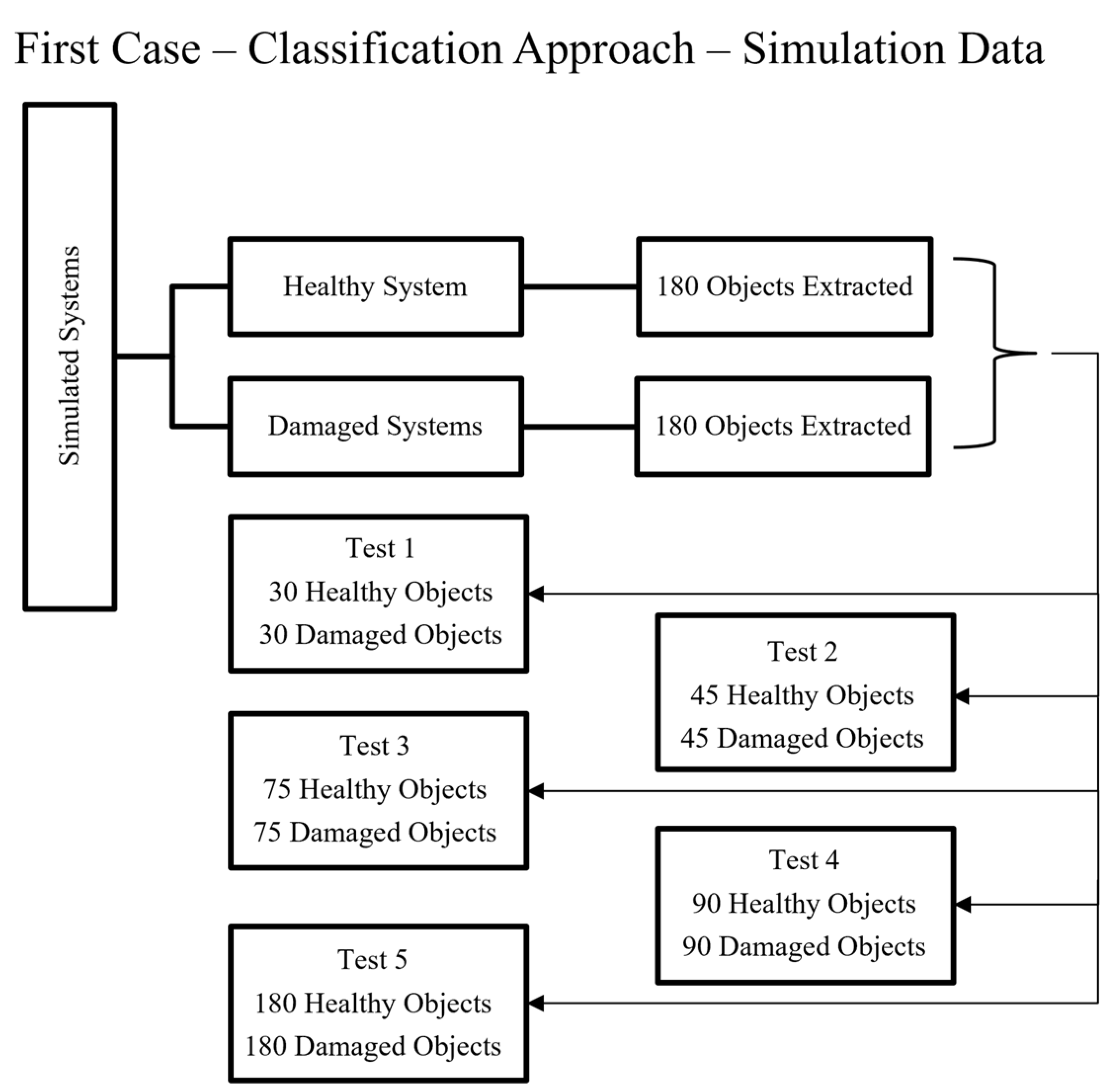
A healthy system and 15 cases of damage (tooth root cracks) were considered in this research (Table 2). Moreover, three cases were exploited. First case: one healthy system and one damaged system (classification case); second case: one healthy and two damaged systems (first multi-class classification case); third case: one healthy and four damaged systems (second multi-class classification case). The tooth root of the spur gear (pinion) with 17 teeth in the test gearbox was used as a reference location for the damage (crack). By disconnecting the elements located in the mesh, with the FE model, the damage can be simulated (Figure 4) [55]. An outlook for the damaged tooth in each condition is visible in Figure 5 for the first classification case and in Figure 6 (damage cases 1 and 2) and Figure 7 (damage cases 3 and 4) for the second multi-class classification case.
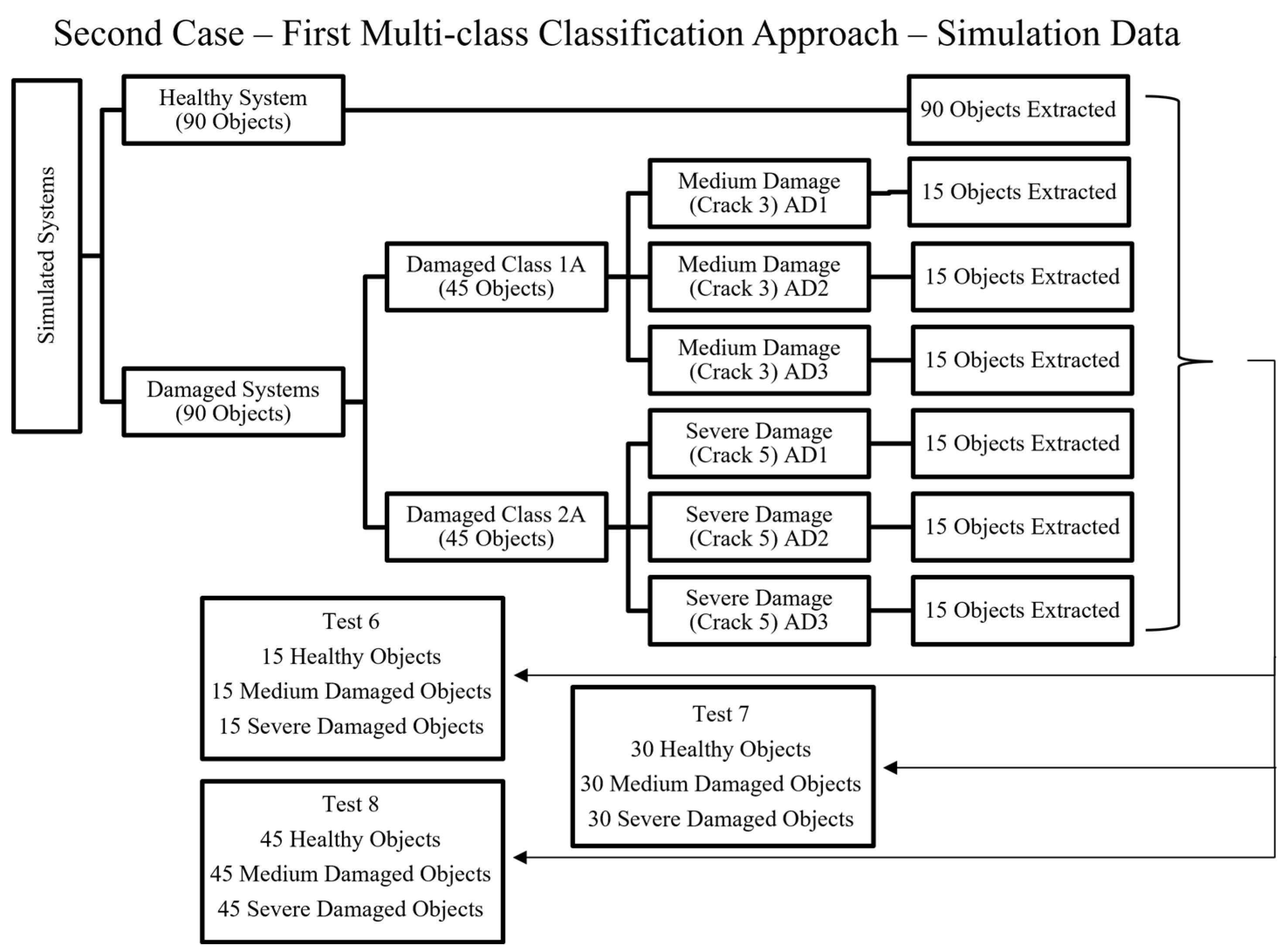
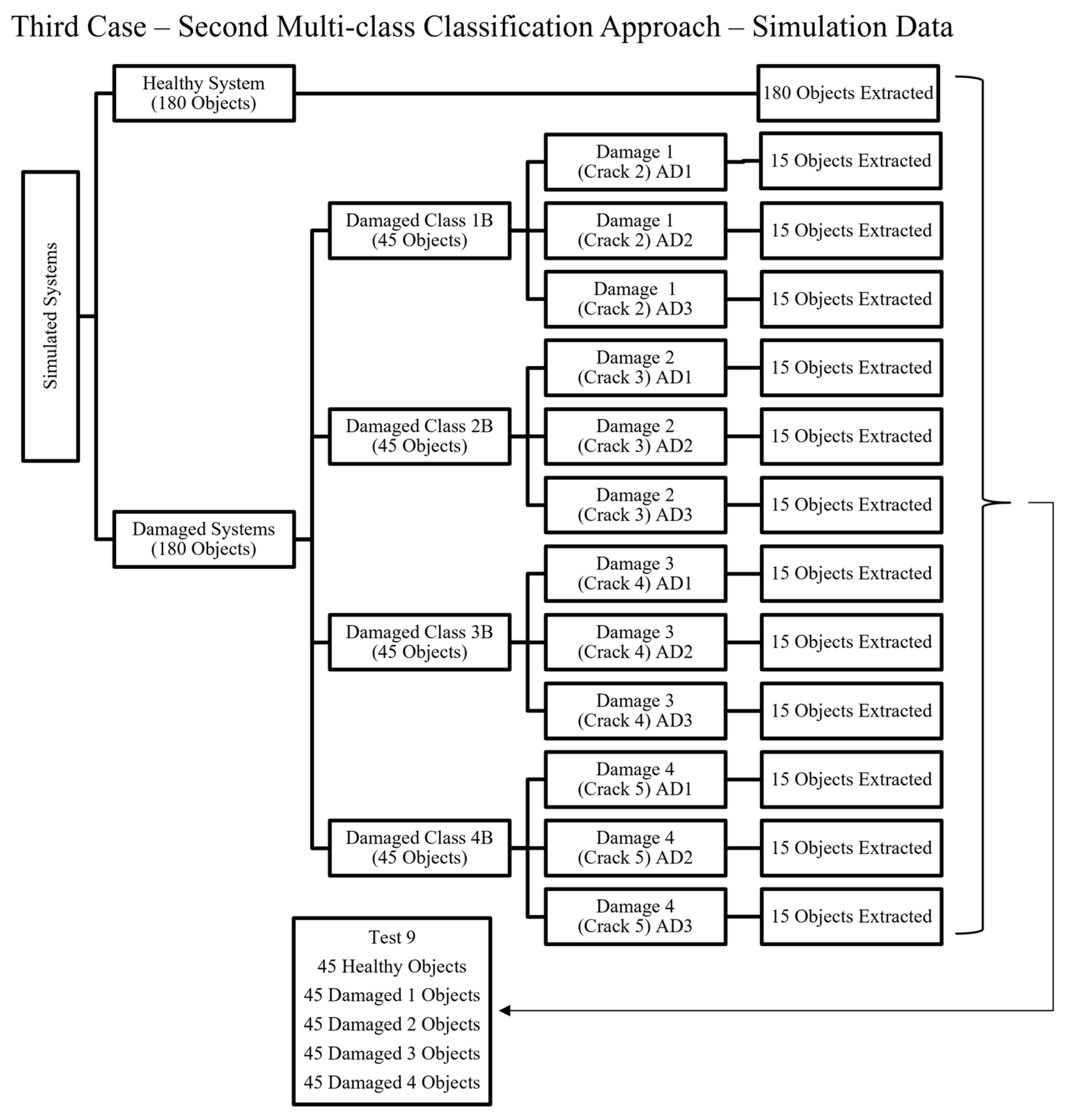
One of the objectives of this research project was to simulate and collect as many data objects as possible from the healthy and damaged systems to use in the ANN approach. The number of extraction points was increased to optimize the results of each simulation. The simulations and data extracted for the first, second, and third cases are visible in Figure 8, Figure 9 and Figure 10, respectively.

3.2. Post-Processing Approach

The locations of the data extracted from the model were selected considering the positions where, on the real test rig, it was feasible to place the piezoelectric accelerometers to collect the signals (gearbox housing), so that it would be possible to validate the simulation results with experimental data. Since the tangential surface of the shaft was the nearest location possible for the housing or bearing seats, this position provided the best-fit option to simulate this signal acquisition [57]. The points that represent the location of each data object extracted are shown in Figure 11. Subsequently, the Fast Fourier Transform (FFT) was applied to each of the data objects—a post-process analysis to check the most common frequencies of the system. In this way, the signal in the time domain represents the vibration responses in a waveform; however, to better visualize the problem, the system behavior was also analyzed in the frequency domain for the classification and multi-class classification problems. Moreover, FFT generates results that allow the visualization of the frequency spread in a spectrum, the energy of which that is carried by a signal can be studied at the frequency determined by the system. Therefore, when some divergence and increment occur in a frequency, damage indicators can be considered in the analysis [58]. Indeed, the FFT can be a good approach for predicting faults. However, it is difficult to determine severity using FFT alone [8]; thus, other sources and techniques, such as ANN, can be used for this purpose.
Moreover, a single numerical simulation took 45 h, approximately, considering 6000 steps, and each object extraction took 4 h. Two seats of the T3D software were used, in which each seat required one computer (RAM: 32GB; Processor: Intel Core i7-11700K) for simulating the system.

4. Artificial Neural Networks (ANNs)

Neural networks are composed of neurons that are connected to each other in a way similar to that in which neurons are connected in a nervous system. What enables this type of system to work properly and in the way that it is intended to is the applicability of the connections that constitute the network [59]. The strong capacity of a neural network can be related to its ability to associate different memories, its high performance in terms of adaptation, and the scope for self-organization and non-linear mapping. All of these indicators are important parameters for solving non-complex problems. ANN is thus a technique that can be widely used in FD [43].
The vibrational spectra that characterize different fault conditions can be processed using ANNs. The training of ANNs can be performed using extracted numerical data; thus, the prediction of damage presence and severity can be completed [60]. After generating a database of simulated signals in healthy and damaged conditions, two types of classification can be performed: binary and multi-class. The determination of the characteristics of a system, in this case healthy and damaged states, should be well performed so that a consistent classification can be made. This procedure can save time and effort when identifying a small set of features [56].
Damage identification was initially the main target of this study, based on ANNs using the classification method followed by damage quantification via the multi-class classification approach. To address this problem, the ANN approach applied here can be activated to identify whether a system has sustained damage or not using pattern recognition. The network is composed of three major elements: input, hidden, and output layers. The Neural Network Pattern Recognition Tool (nprtool), in MATLAB, was used to construct the architecture. It is an effective tool when the data can be inaccurate or incomplete [61]. Additionally, the hidden layer (referred to as neurons) uses a sigmoid activation function. In this way, the specific output is produced by the mathematical functions raised from the sigmoid function. Then, a linear function is used by the output. In the hidden layer of signal processing nodes, the number of neurons can be equal to one or more, depending on the ANN architecture characteristics and its number of objects [62].
Hyper-parameters are known by their characteristics consisting of the number of hidden layers and neurons in the data frame. Each neuron of layer L is connected to each neuron of layer L + 1 . Then, a value can be assigned to the neurons according to the weight matrix. Hyper-parameters are applied to create, visualize, and train two-layer feedforward networks to solve data classification problems.
For the network to achieve the target value, a relative non-linearity can be introduced inside the function. In this way, the output function can be predicted and, after that, an error that occurred after training can be constantly pursued by the network. The propagation of the prediction goes back to the networks, using the Back Propagation (BP) learning algorithm. This happens when the prediction is wrong and the stochastic gradient descendant method is used to find the gradient error [34].
The first part of the analysis aims at the characterization of damage (classification), which is represented in Figure 12. The second set of analyses aim at the definition of damage severity (multi-class classification), which is represented in Figure 13.
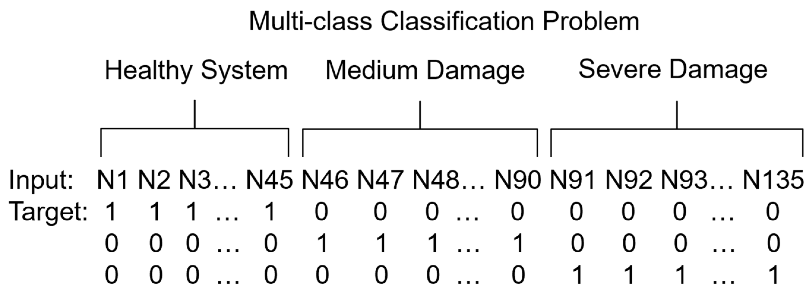
The first step in implementing this approach was to define the best way to organize the data as input objects and targets to build a good ANN architecture. Then, since the frequency steps, at the spectra obtained through numerical simulation and after FFT, are the same for all healthy and damaged systems, the amplitudes of each frequency component were used as input attributes for this analysis because these are the features that differentiate each case. The input data are organized in a data table, where each column is an object (a simulation signal) and each row is a dimension of these objects. In this case, each frequency component of the spectrum is considered as a dimension, while the target file is composed of rows of zeros and ones, in which zeros are labels that correspond to the healthy system and ones to the damaged system by using this type of classifier (Figure 14). Hence, this classification problem is used to characterize the system as damaged or undamaged, only. On the other hand, the multi-class classification problem is used to characterize the severity of the damage. This can be achieved due to the one-hot encoding, which is a method that converts the data for better ANN algorithm performance. In this work, categorical variables are converted into unique binary numbers to be used in multiple classifications, defining the healthy system and cases of damage as medium or severe cases. Indeed, to make a classifier algorithm more efficient, transformation of the data characteristics of any entity into vectors of binary numbers is required [63]. In this way, the input file is constructed essentially in the same way as in the previous example; however, the target file is differently created. It is composed of a table in which each column is a unique vector, where the position of the number one represents a class (healthy, medium-level damaged, or severely damaged system), as shown in Figure 15.
The features of this “nprtool” tool are very intuitive, enabling the user to efficiently create a good ANN architecture. While the network is being trained, a percentage of the input data can be allocated to validation and testing. Moreover, the ANN “nprtool” automatically mixes data from each healthy and damaged system category to randomize the order of the objects. The system process consists of training, validation, and testing phases. Then, more precise results can be expected since the process is undergoing correction during the training phase and stops when it reaches the minimum error. Additionally, validation can be the factor that stops the process after the network reaches a satisfying accuracy when recognizing an object. To guarantee a sufficient success capability of the trained algorithm, a procedure suitable for the optimization of the ANN structure and the evaluation of its performance in terms of damage diagnosis was used, thus avoiding data overfitting, even given the limited number of examples [54]. Indeed, overfitting occurs when a model learns the detail and noise in the training data. It usually negatively impacts the performance of the model with respect to new data, since the noise or random fluctuations in the training data are learned as concepts by the ANN model. In addition, overfitting tends to be influenced by non-parametric and nonlinear models, which have more flexibility in learning a target function. Thus, ANNs are non-parametric. However, ANNs are practical to use, and the accuracy of neural classifiers is high. In addition, they include parameters to limit and constrain the quantity of details the model can learn to reduce overfitting.
For the FD of rotating machines, it is not necessary to have deep knowledge about the behavior of the rotating machine and the operation of its internal mechanisms. This proves to be a significant advantage in this type of diagnosis, while a disadvantage can be the large number of boxing examples required for the analysis [61]. Considering this, examples of important parameters from the “nprtool” interface (MATLAB ver. R2020b) that allow the user to have total control of the training process are presented in Table 3.

5. Results

The numerical analysis aimed at the extraction of displacements and, after a double integration, the extraction of vibrations. The time discretization (sampling) must be selected accurately for the performance of the extraction. To avoid aliasing phenomena, the time discretization should be enough dense; however, at the same time, it should be conserved as far as possible to limit the computational effort. Moreover, the time-step, which defines the resolution of the analysis, can be affected by the rotational speed of the system, the number of teeth, the number of meshing pairs, the number of harmonics, and the number of time-steps for each meshing period [43]. In this regard, GMFs can be used to determine the sampling time of the analysis.
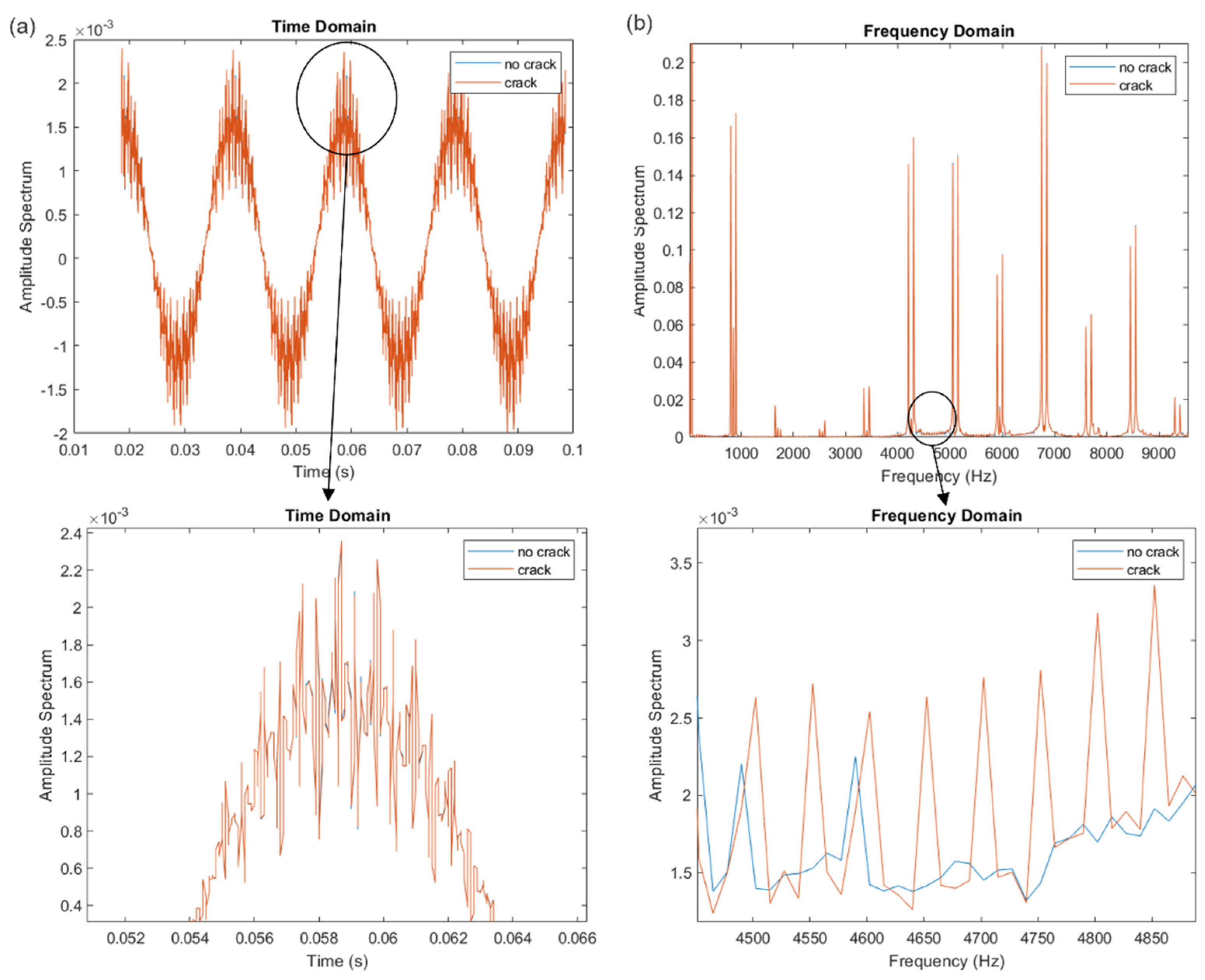
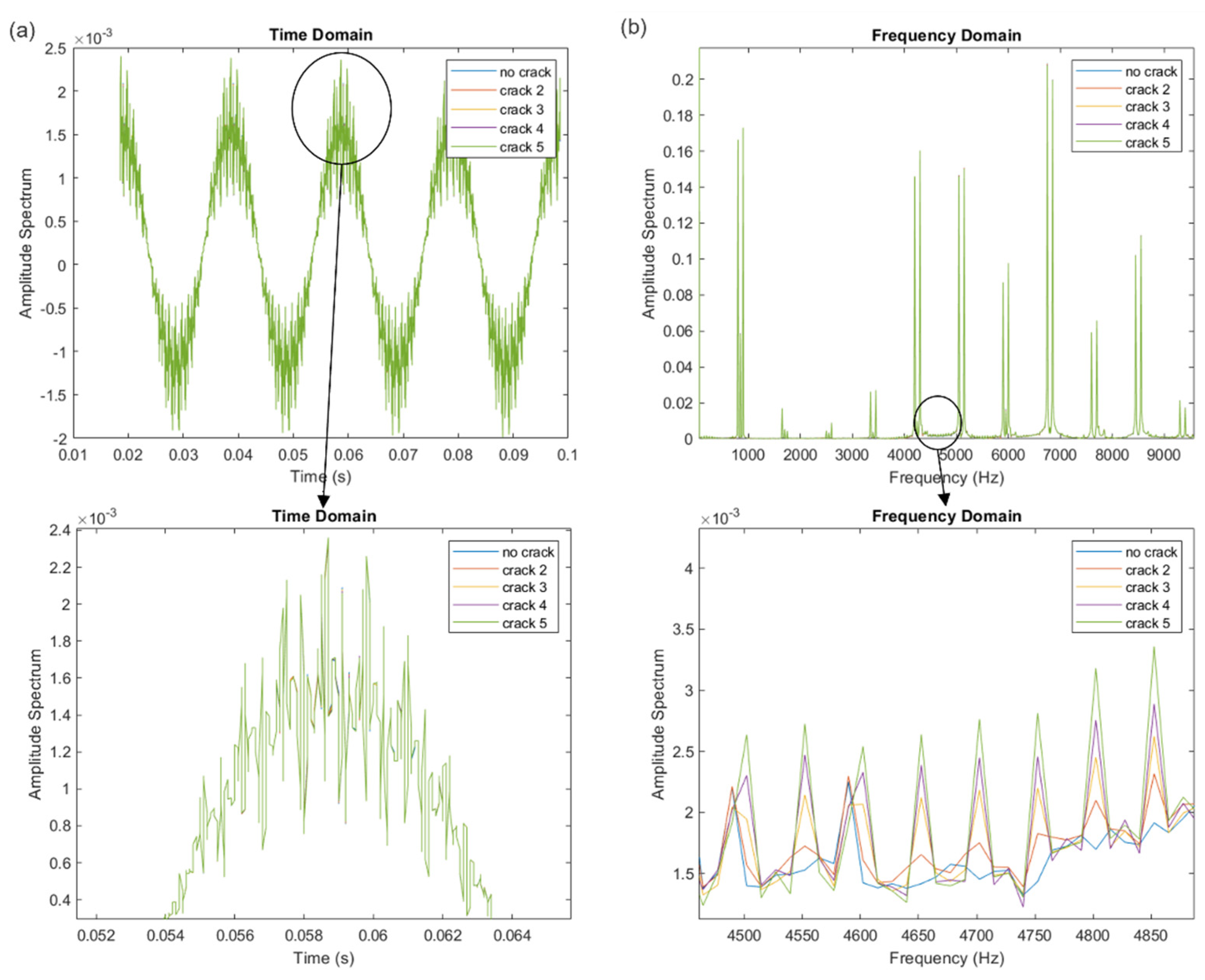
After post-processing the data, the GMFs of the system (Spur Gear Pair: 850 Hz; Helical Gear Pair: 1700 Hz) are visible. Peaks of 50 Hz away from each other were visibly found in the spectra for all simulated systems. They have a sharp definition in the damaged systems, whose amplitudes at each peak became higher each time the damage level was increased. This was expected. Examples of some of the signals in the time and frequency domains are shown in Figure 16a,b for the classification problem and in Figure 17a,b for the multi-class classification problem. The system simulation considers five harmonics, which gives the possibility of observing frequencies in the range of 8500 Hz.
The sideband is another important feature in this analysis. Since the wave generated by the meshing gears is generally not a pure sinusoidal function, because the relative amplitude of the different harmonics determines the quality of the sinusoidal wave, the spectra usually show additional harmonics of the GMFs with their own sideband group. Then, all real sinusoidal waves can have some number of harmonics present in each one. Thus, when determining two or more complex sinusoidal waves, it must be seen whether any pair of harmonics lies within a critical bandwidth. In fact, producing a pure wave is rather difficult because it is very hard to remove all of these clustered harmonics, which may cause noise signals. Therefore, in a healthy system, the amplitude of the side bands can be low, while in damaged cases the sidebands increase due to the vibrational spectra, which increasingly differ from the ideal sine function.
Since the first ANN approach applied in this research was the classification to determine systems with no damage and with damage conditions (Figure 7), the first case was used. Initially, systems exhibiting healthy or damage behavior, with only one element, were simulated. However, considering that the one-element damage signal has a very low amplitude spectrum compared to severe damage due to a low-level crack, the damage signals presented features very similar to the healthy system features. This similarity resulted in an ANN that was unable to recognize these data as signifying damage. Therefore, one-element damage was not considered for the ANN training.
Hence, one dataset of simulated data for the first case was created to train an ANN model, called Test 1, to observe the responses of this first training set. Test 1 consisted of 30 signals from a healthy system and 30 signals from a damaged system. However, due to the limited number of data, the responses for this test were unsatisfactory. For Test 1 (60 objects in total), the results of the confusion matrix are presented in Figure 18, while the best validation performance, error histogram, and training state plots are presented in Figure 19. Considering the previous result, four different datasets for the first case, with more simulated data, were created to train four different ANN models with the same architecture. These datasets were called Test 2, Test 3, Test 4, and Test 5. Test 2 consisted of 45 signals for the healthy system and 45 signals for the damaged system; Test 3 consisted of 75 signals for the healthy system and 75 signals for the damaged system; Test 4 consisted of 90 signals for the healthy system and 90 signals for the damaged system; and Test 5 consisted of 180 signals for the healthy system and 180 signals for the damaged system. For Test 2 (90 objects in total), the results of the confusion matrix are presented in Figure 20, while the best validation performance, error histogram, and training state plots are presented in Figure 21. For Test 3 (150 objects in total), the results of the confusion matrix are presented in Figure 22, while the best validation performance, error histogram, and training state plots are presented in Figure 23. For Test 4 (180 objects in total), the results of the confusion matrix are presented in Figure 24, while the best validation performance, error histogram, and training state plots are presented in Figure 25. For Test 5 (360 objects in total), the results of the confusion matrix are presented in Figure 26, while the best validation performance, error histogram, and training state plots are presented in Figure 27. The damage category used for the Tests 2, 3, 4, and 5 architectures considered sorted objects extracted from cracks 2, 3, 4, and 5.
Then, to classify the severity of system damage, two more cases were considered. The architecture of the second case (first multi-class classification approach) could determine the state of the system under three conditions: no damage, medium damage (crack 3), and severe damage (crack 5), as shown in Figure 9. On the other hand, the architecture of the third case (second multi-class classification approach) could determine the state of the system in five conditions: no damage, damage 1 (crack 2), damage 2 (crack 3), damage 3, (crack 4), and damage 4 (crack 5), as shown in Figure 10.
For the second case, one dataset, called Test 6, was created to train an ANN model. Test 6 consisted of 15 signals of a healthy system, 15 signals of a medium-damaged system, and 15 signals of a severely damaged system. However, due to the limited number of data, the responses for this test were unsatisfactory. For Test 6 (45 objects in total), the results of the confusion matrix are presented in Figure 28, while the best validation performance, error histogram, and training state plots are presented in Figure 29. Then, two datasets of simulated data, called Test 7 and Test 8, were created to train two different ANN models with the same architecture. Test 7 consisted of 30 signals for a healthy system, 30 signals for a medium-damaged system, and 30 signals for a severely damaged system, while Test 8 consisted of 45 signals for a healthy system, 45 signals for a medium-damaged system, and 45 signals for a severely damaged system. For Test 7 (90 objects in total), the results of the confusion matrix are presented in Figure 30, while the best validation performance, error histogram, and training state plots are presented in Figure 31. For Test 8 (135 objects in total), the results of the confusion matrix are presented in Figure 32, while the best validation performance, error histogram, and training state plots are presented in Figure 33. The medium damage category used for the Test 6, Test 7, and Test 8 architectures considered objects extracted from crack 3 (Damage Class 1A), only, while the severe damage category used for the Test 6, Test 7, and Test 8 architectures considered objects extracted from crack 5 (Damage Class 2A), only (Figure 9).
For the third case, one dataset of simulated data, called Test 9, was created. Test 9 consisted of 45 signals for a healthy system, 45 signals for a damage 1 system (crack 2), 45 signals for a damage 2 system (crack 3), 45 signals for a damage 3 system (crack 4), and 45 signals for a damage 4 system (crack 5). For Test 9 (225 objects in total), the results of the confusion matrix are presented in Figure 34, while the best validation performance, error histogram, and training state plots are presented in Figure 35. The damage 1 category used for the Test 9 architecture considered objects extracted from crack 2 (Damage Class 1B), only; the damage 2 category considered objects extracted from crack 3 (Damage Class 2B), only; the damage 3 category considered objects extracted from crack 4 (Damage Class 3B), only; and the damage 4 category considered objects extracted from crack 5 (Damage Class 4B), only (Figure 10).

6. Discussion

After obtaining the responses of the system in healthy and damaged conditions, it was observed that specific frequencies, between the range of 0 Hz and 8500 Hz, due to the harmonics considered in this work, shift given the presence of damage [50]. Indeed, the results in terms of signals from the healthy system could be validated with the signals from the experimental test. In view of this, a vector was created to organize the input data for the ANN approach. Since the dimension of the analysis (extracted objects from each simulation) went from 100 Hz to 10,000 Hz, the classification method could identify whether a system has damage or not, and the multi-class classification method could recognize the severity of the damages identified. The characteristics and algorithm performances for each test for the classification and multi-class classification methods can be found below.
The classification approach consisted of Tests 1, 2, 3, 4, and 5. The total number of observations (objects) and the percentage are exposed in each cell of the confusion matrixes, whose characteristics are related to the demonstration of the actual value and the predicted value. The confusion matrix rows correspond to the output class (true class), which are 0 (no damage) and 1 (damage), while the columns correspond to the target class (predicted class), which are 0 (no damage) and 1 (damage). The main diagonal elements represent the classified samples (correct observations), while the off-diagonal elements correspond to the misclassified samples (wrong observations) [64]. To better visualize the problem regarding the “All Confusion Matrix” of Test 5 (the best performance model for the classification method achieved in this work), as shown in Figure 26, its results characteristics can be seen in Table 4, whose parameters and values are explained [65]. For Tests 1, 2, 3, 4, and 5, the network took 14, 19, 18, 28, and 18 epochs (training state plots) to train and validate the model, respectively. Performance per epoch has indicators of Cross-Entropy (CE) and Errors (%E). CE operation computes the CE loss between network predictions and target values for single-label classification tasks. Its value also shows the efficiency of the network, while the %E shows the fraction of predictions misclassified (Table 3). When the CE of the validation phase reaches the minimum value, this is considered the best mark of the training phase, because overfitting occurs from that point. It is possible to observe this characteristic due to the fact that the training curve continues to decrease, while the validation curve starts to increase. Thus, it is possible to observe when the overfitting starts in this part of the plot. Moreover, the “nprtool” takes this value index, whose function shows the best possible result for this ANN architecture. In addition, when the validation sampling of input data reaches the lowest CE of the last six epochs, the network (validation) stops training when the non-training validation subset error rate increases continuously for more than six (default) epochs. This can be seen in the training state plots. Considering this, the performance for Test 5 was better than the performance for Tests 1, 2, 3, and 4. When errors between the target values and predicted values appear after the training of a network, the histogram can be used. Then, the Error Histogram has the capacity to show the differences between predicted values and target values. Moreover, an ANN with histogram features is highly recommended for FD in gearboxes [64]. Therefore, by analyzing the detection performances of the confusion matrix and the plots of the best validation performance, error histogram, and training state, for classification problems (Tests 1, 2, 3, 4, and 5), Test 5 was considered the best model. This performance result can be explained by the greater number of objects used in the network compared to the other models.
The first case of the multi-class classification approach consists of Tests 6, 7, and 8. As well as the multi-class approach, the total number of observations (objects) in each cell and its percentage are exposed in the confusion matrixes. However, the rows and columns are different. The confusion matrix rows for the multi-class classification problem correspond to the output class (true class), which are 1 (no damage), 2 (medium damage), and 3 (severe damage), while the columns correspond to the target class (predicted class), which are 1 (no damage), 2 (medium damage), and 3 (severe damage). To better visualize the problem regarding the “All Confusion Matrix” of Test 8 (the best performance model for the multi-class classification method—first case achieved in this work), as shown in Figure 32, its results characteristics can be seen in Table 5, the parameters and values in which are explained [65]. For Test 6, 7, and 8, the network took 13, 30, and 50 epochs (training state plots) to train and validate the model, respectively. When the CE of the validation phase reaches the minimum value, this is considered the best mark of the training phase, because overfitting occurs from that point, similarly to the previous classification problem case. Hence, the performance of Test 8 was considered better than those of Tests 6 and 7. The errors visualized in the Error Histogram for Test 8 were low compared to the other tests. Therefore, by analyzing the detection performances of the confusion matrix and the plots of the best validation performance, error histogram, and training state, for multi-class classification problems (Tests 6, 7, and 8), Test 8 was considered the best model and, once again, this performance result can be explained by the greater number of objects used in the network compared to the other models.
The second case of the multi-class classification approach consists of Test 9. The rows of the confusion matrix for this multi-class classification problem correspond to the output class (true class), which are 1 (no damage), 2 (damage 1), 3 (damage 2), 4 (damage 3), and 5 (damage 4), and the columns correspond to the target class (predicted class), which are 1 (no damage), 2 (damage 1), 3 (damage 2), 4 (damage 3), and 5 (damage 4). For Test 9, the network took 54 epochs (training state plot) to train and validate the model (Figure 35). By analyzing the plot, when the CE of the validation phase reaches the minimum value, this is considered the best mark of the training phase because overfitting occurs from that point. CE is high when the number of epochs is low, and when the number of epochs expands, the loss function is reduced. Therefore, the performance of Test 9 was considered satisfactory, even when using a limited number of objects to create the architecture.
By analyzing these different ANN models and their responses, it can be noted that the more objects used, the higher the chance of creating a good ANN architecture.

7. Conclusions

Since the SHM has the capability of maintaining a system through online monitoring, which provides an efficient procedure for continuous inspection of a system, experimental configuration can be an option to implement SHM. However, due to the costs involved, it can be impracticable. Thus, the solution proposed in this work was the implementation of a model-based approach, the data for which can be used for the SHM. These data were generated from numerical models, simulated through a hybrid FEM–analytical approach, and used for the implementation of the ANNs (SHM technique).
For the test rig, a reference geared system, the hybrid FEM–analytical approach proved to be an efficient method for performing simulations of healthy and damaged systems, as a result of the low computational effort as compared to other methods and the accurate reproduction of the real geometric model. This is due to the analytical solution developed with a few equations. Furthermore, it was found that a satisfactory performance of the method related to each active contact, in the operation of the mechanical test bench system, was obtained even with the solution with a relatively coarse grid. Since the contacts are solved through analytical equations (based on Hertzian theory), the numerical FE model was developed to evaluate the responses in the contacts related to the forces present in the system, considering the macro-deflections in the components of the mechanism. Indeed, the contact pressures between the analyzed mechanisms are estimated. Furthermore, this approach does not require a mesh refinement to properly simulate contact and provide convergence to the simulation in the same way as a traditional FEM. Hence, this proves even more that the hybrid FEM–analytical approach is more viable, because the simulation of a real system, composed of several mechanical and rotating components, can be completely developed. Since the novelty of this work is associated with the model-based numerical approaches that are simulated in healthy and damaged conditions, the lack of need for geometrical simplifications makes the computational effort, for the approach, relatively low. In addition, the investigation of damages in terms of the health state of a system, as a new aspect, was employed in this work by adding different positions and dimensions to the cracks on the tooth root of the spur gear.
The signal resolution of the overall data acquired was consistent, given all pre-process and post-process configurations from the numerical simulation techniques. The spectra, after adjustment of the sampling data and frequency range, showed the characteristics and differences between the healthy and damaged systems, beyond the clearness of the signals acquired. These predicted the visualization of the GMFs of the system (850 and 1700 Hz), the five harmonics (1700 × 5 Hz), the sidebands and the peaks of 50 Hz, especially for the damaged systems. Moreover, separating the gearbox-related signal (a pure sinusoidal wave) from other components can be quite complicated. However, this was done to minimize noise that can interfere with the responses related to the gearbox signal. Therefore, this can be investigated to reduce the alteration of the signal from one affected component to the signal from other analyzed ones.
The responses of the ANN models were adequate due to the resulting accuracy achieved after post-processing each object from the FEM simulations. Even considering the limited number of objects for these ANN architectures, the resulting accuracy observed in the plots, especially in the All Confusion Matrix for each ANN model, was demonstrated to be extremely satisfactory. This was possible to achieve by using several different points for data extraction from each simulation in order to have more objects than simulations. Indeed, analyzing histogram plots and their features for ANN models is highly recommended for FD in gearboxes.
For the first case (the classification approach), Test 5 presented the best performance model, while for the second case (the first multi-class classification approach), Test 8 presented the best one. The results for Test 9, which was the third case (the second multi-class classification approach), were consistent with the results for the previous cases due to the good prediction performance of the algorithm, even when using a limited number of objects for each case of damage. Moreover, overfitting may arise, given the limited amount of data acquired by FEM simulations that were used to construct the database. However, even with the restriction of usable data for the ANN architecture, the results obtained were coherent with respect to the examined scenario. Furthermore, the “nprtool” was able to avoid overfitting by using the validation dataset, since the “nprtool” algorithm separated part of the objects for the validation phase, which is not always done, yet it is strongly recommended. Then, the percentage of all confusion matrixes, from each ANN model (Tests 5, 8, and 9), which identified the system characteristics, considering the training, validation, and test performance, indicated that these models predicted well the planned initial idea. Test 5 classifies well whether the system has damage or not (classification approach). Test 8 and Test 9 classify well whether the system has damage or not in addition to the severity of damage that can be predicted (multi-class classification approaches). Thus, these results show how well the classification model performs and what kinds of errors it makes.
Even requiring a long time for the dynamic FEM simulations (still more viable than a traditional FEM), post-processing of the results, and performance of the ANN technique, this methodology was suitable and consistent for the test bench presented in this paper. Moreover, this methodology is valid for other types of test rig configurations, considering that the implementation of their digital models and creation of their databases should be carried out.
The accuracy of the ANN models can yield even better responses if more objects are extracted from the FEM simulations and used to train the ANN. Indeed, this can be applied to the one-element damage example, the analysis of which was considered unfeasible for the current research paper because its ANN model was unable to recognize whether the data (extracted signals from the healthy and damaged systems) signified a damaged or an undamaged system. Thus, for future studies, to complement and advance the research in relation to damage severity, more damage simulations for positions related to all axial dimensions analyzed here could be performed. On the other hand, another possibility is the addition of multiple damage conditions, separately or simultaneously, to the crack on the tooth root of the spur gear. Then, by collecting more objects from these different cases of damage from FEM simulations, other ANN models could be developed to identify more locations and severities of damage in order to characterize and create a robust SHM system.

Author Contributions

Conceptualization: all; methodology: all; formal analysis, implementation, data curation, and validation: R.d.P.M. and A.L.M.; resources: R.V., F.C. and C.G.; writing—original draft preparation: R.d.P.M.; writing—review and editing: all; supervision, R.V., F.C. and C.G. All authors have read and agreed to the published version of the manuscript.

Funding

This research received no external funding.

Institutional Review Board Statement

Not applicable.

Informed Consent Statement

Not applicable.

Data Availability Statement

The datasets used and/or analyzed during the current study are available from the corresponding author upon reasonable request.

Conflicts of Interest

The authors declare no conflict of interest.

Abbreviations

ADAxial Dimension
AIArtificial Intelligence
ANNArtificial Neural Network
BPBack Propagation
CECross-Entropy
CMCondition Monitoring
DLDeep Learning
FDFault Diagnosis
FEFinite Element
FEMFinite Element Method
FFTFast Fourier Transform
FMDFalse Medium Damage
FNFalse Negative
FNDFalse No Damage
FPFalse Positive
FSDFalse Severe Damage
FZGForschungsstelle fur Zahnrader und Getriebebau
GMFGear Mesh Frequency
MLMachine Learning
nprtoolNeural Network Pattern Recognition
RAMRandom Access Memory
RDRadial Dimension
SHMStructural Health Monitoring
TMDTrue Medium Damage
TNTrue Negative
TNDTrue No Damage
TPTrue Positive
TSDTrue Severe Damage
T3DTransmission3D
%EPercent Error
Nomenclature
a Actual objects
bFace width
C d Center distance
d p Pitch circle diameter
E Young’s modulus
J Moment of inertia
L Neuron layer
m Mass
m n Normal module
N Total number of objects
P Predicted objects
q Point inside the solid body
r Field point r
r i j Surface grid point
r m i n Rotational speed
u ( r i j ; r ) Displacement due to a load at the surface grid
ν Poisson’s ratio
z Number of teeth
z m i n Number of teeth
α n Pressure angle
β Helix angle
ε Contact ratio

References

  1. Monteiro, R.P.; Vidoni, R.; Concli, F. A Multibody Dynamic Model for Evaluating the Vibrating Modes of Gear Train Systems. Int. J. Transp. Dev. Integr. 2021, 5, 264–277. [Google Scholar] [CrossRef]
  2. Marra, A.L.; Juliani, R.; Garcia, C. Data Augmentation for Vibration Signals using System Identification Techniques. In Proceedings of the 2021 5th International Conference on System Reliability and Safety (ICSRS), Palermo, Italy, 24–26 November 2021. [Google Scholar] [CrossRef]
  3. Nentwich, C.; Reinhart, G. A Method for Health Indicator Evaluation for Condition Monitoring of Industrial Robot Gears. Robotics 2021, 10, 80. [Google Scholar] [CrossRef]
  4. Wang, D.; Tsui, K.-L.; Miao, Q. Prognostics and Health Management: A Review of Vibration Based Bearing and Gear Health Indicators. IEEE Access 2018, 6, 665–676. [Google Scholar] [CrossRef]
  5. Sendlbeck, S.; Fimpel, A.; Siewerin, B.; Otto, M.; Stahl, K. Condition Monitoring of Slow-speed Gear Wear using a Transmission Error-based Approach with Automated Feature Selection. Int. J. Progn. Health Manag. 2021, 12, 2. [Google Scholar] [CrossRef]
  6. Chen, X.; Semenov, S.; McGugan, M.; Madsen, S.H.; Yeniceli, S.C.; Berring, P.; Branner, K. Fatigue testing of a 14.3 m composite blade embedded with artificial defects Damage growth and structural health monitoring. Compos. Part A Appl. Sci. Manuf. 2020, 140, 106189. [Google Scholar] [CrossRef]
  7. Zhang, K.; Yang, Z. Identification of Load Categories in Rotor System Based on Vibration Analysis. Sensors 2017, 17, 1676. [Google Scholar] [CrossRef] [PubMed] [Green Version]
  8. Kumar, S.; Lokesha, M.; Kumar, K.; Srinivas, K.R. Vibration based Fault Diagnosis Techniques for Rotating Mechanical Components: Review Paper. IOP Conf. Ser. Mater. Sci. Eng. 2018, 376, 012109. [Google Scholar] [CrossRef]
  9. Toh, G.; Park, J. Review of Vibration-Based Structural Health Monitoring Using Deep Learning. Appl. Sci. 2020, 10, 1680. [Google Scholar] [CrossRef]
  10. Woo, S. Reliability Design of Mechanical Systems. A Guide for Mechanical and Civil Engineers, 2nd ed.; Springer: Singapore, 2020; ISBN 978-981-13-7236-0. [Google Scholar] [CrossRef]
  11. Aherwar, A. An investigation on gearbox fault detection using vibration analysis techniques: A review. Aust. J. Mech. Eng. 2012, 10, 169–183. [Google Scholar] [CrossRef]
  12. Zhou, Y.; Zhu, C.; Liu, H.; Bai, H.; Xu, X. Investigation on stress microcycles and mild wear mechanism in gear contact fatigue. Fatigue Fract. Eng. Mater. Struct. 2021, 44, 2265–2279. [Google Scholar] [CrossRef]
  13. Chen, X.; Yang, X.; Zuo, M.; Tian, Z. Planetary Gearbox Dynamic Modeling Considering Bearing Clearance and Sun Gear Tooth Crack. Sensors 2021, 21, 2638. [Google Scholar] [CrossRef] [PubMed]
  14. Liu, H.; Liu, H.; Zhu, C.; Sun, Z.; Bai, H. Erratum to: Study on contact fatigue of a wind turbine gear pair considering surface roughness. Friction 2019, 10, 1135. [Google Scholar] [CrossRef] [Green Version]
  15. Xiao, Z.; Cao, J.; Yu, Y. Mathematical Modeling and Dynamic Analysis of Planetary Gears System with Time-Varying Parameters. Math. Probl. Eng. 2020, 2020, 3185624. [Google Scholar] [CrossRef] [Green Version]
  16. Wang, T.; Han, Q.; Chu, F.; Feng, Z. Vibration based condition monitoring and fault diagnosis of wind turbine planetary gearbox: A review. Mech. Syst. Signal Process. 2019, 126, 662–685. [Google Scholar] [CrossRef]
  17. Allam, A.; Moussa, M.; Tarry, C.; Veres, M. Detecting Teeth Defects on Automotive Gears Using Deep Learning. Sensors 2021, 21, 8480. [Google Scholar] [CrossRef]
  18. Li, D.; Zhang, S.; Yang, W.; Zhang, W. Corrosion Monitoring and Evaluation of Reinforced Concrete Structures Utilizing the Ultrasonic Guided Wave Technique. Int. J. Distrib. Sens. Netw. 2014, 10, 827130. [Google Scholar] [CrossRef]
  19. Sridhar, V.; Chana, K. Development of a Novel Sensor for Gear Teeth Wear and Damage Detection. Int. J. Progn. Health Manag. 2021, 12, 3. [Google Scholar] [CrossRef]
  20. Teng, W.; Ding, X.; Tang, S.; Xu, J.; Shi, B.; Liu, Y. Vibration Analysis for Fault Detection of Wind Turbine Drivetrains—A Comprehensive Investigation. Sensors 2021, 21, 1686. [Google Scholar] [CrossRef] [PubMed]
  21. Aherwar, A.; Khalid, S. Vibration analysis techniques for gearbox diagnostic: A review. Int. J. Adv. Eng. Technol. 2012, 3, 4–12. [Google Scholar]
  22. Alwadie, A.; Muhammad, I.; Nordin, S. The Fault Detection of Gear of Electromechanical Power Transmission System using Frequency Domain Approach. Renew. Energy Power Qual. J. 2021, 19. [Google Scholar] [CrossRef]
  23. Civera, M.; Surace, C. A Comparative Analysis of Signal Decomposition Techniques for Structural Health Monitoring on an Experimental Benchmark. Sensors 2021, 21, 1825. [Google Scholar] [CrossRef] [PubMed]
  24. Wah, W.S.L.; Chen, Y.-T.; Owen, J.S. A regression-based damage detection method for structures subjected to changing environmental and operational conditions. Eng. Struct. 2020, 228, 111462. [Google Scholar] [CrossRef]
  25. Chandrasekhar, K.; Stevanovic, N.; Cross, E.J.; Dervilis, N.; Worden, K. Damage detection in operational wind turbine blades using a new approach based on machine learning. Renew. Energy 2020, 168, 1249–1264. [Google Scholar] [CrossRef]
  26. Schmidt, S.; Heyns, P.S.; Gryllias, K.C. An informative frequency band identification framework for gearbox fault diagnosis under time-varying operating conditions. Mech. Syst. Signal Process. 2021, 158, 107771. [Google Scholar] [CrossRef]
  27. Cao, X.; Rembe, C. Non-Contact Damage Detection under Operational Conditions with Multipoint Laservibrometry. Sensors 2020, 20, 732. [Google Scholar] [CrossRef] [PubMed] [Green Version]
  28. Lu, K.; Gu, J.X.; Fan, H.; Sun, X.; Li, B.; Gu, F. Acoustics Based Monitoring and Diagnostics for the Progressive Deterioration of Helical Gearboxes. Chin. J. Mech. Eng. 2021, 34, 1–12. [Google Scholar] [CrossRef]
  29. Salameh, J.P.; Cauet, S.; Etien, E.; Sakout, A.; Rambault, L. Gearbox condition monitoring in wind turbines: A review. Mech. Syst. Signal Process. 2018, 111, 251–264. [Google Scholar] [CrossRef]
  30. Ravikumar, K.; Madhusudana, C.; Kumar, H.; Gangadharan, K. Classification of gear faults in internal combustion (IC) engine gearbox using discrete wavelet transform features and K star algorithm. Eng. Sci. Technol. Int. J. 2022, 30, 101048. [Google Scholar] [CrossRef]
  31. Chen, W.; Dai, S.; Zheng, B. ARIMA-FEM Method with Prediction Function to Solve the Stress–Strain of Perforated Elastic Metal Plates. Metals 2022, 12, 179. [Google Scholar] [CrossRef]
  32. Rossi, M.; Renzi, M. A general methodology for performance prediction of pumps-as-turbines using Artificial Neural Networks. Renew. Energy 2018, 128, 265–274. [Google Scholar] [CrossRef]
  33. Surendran, R.; Khalaf, O.I.; Romero, C.A.T. Deep Learning Based Intelligent Industrial Fault Diagnosis Model. Comput. Mater. Contin. 2022, 70, 6323–6338. [Google Scholar] [CrossRef]
  34. Singh, V.; Gangsar, P.; Porwal, R.; Atulkar, A. Artificial intelligence application in fault diagnostics of rotating industrial machines: A state-of-the-art review. J. Intell. Manuf. 2021, 1–30. [Google Scholar] [CrossRef]
  35. Lei, Y.; Yang, B.; Jiang, X.; Jia, F.; Li, N.; Nandi, A.K. Applications of machine learning to machine fault diagnosis: A review and roadmap. Mech. Syst. Signal Process. 2020, 138, 106587. [Google Scholar] [CrossRef]
  36. Dworakowski, Z.; Dziedziech, K.; Jabłonski, A. A novelty detection approach to monitoring of epicyclic gearbox health. Metrol. Meas. Syst. 2018, 25, 459–473. [Google Scholar] [CrossRef]
  37. Cao, R.; Yunusa-Kaltungo, A. An Automated Data Fusion-Based Gear Faults Classification Framework in Rotating Machines. Sensors 2021, 21, 2957. [Google Scholar] [CrossRef] [PubMed]
  38. Ahmed, R.; Pai, P.S.; Sriram, N.; Bhat, V. Comparison of wavelet based denoising schemes for gear condition monitoring: An Artificial Neural Network based Approach. IOP Conf. Ser. Mater. Sci. Eng. 2018, 310, 012010. [Google Scholar] [CrossRef]
  39. Strączkiewicz, M.; Barszcz, T. Application of Artificial Neural Network for Damage Detection in Planetary Gearbox of Wind Turbine. Shock Vib. 2016, 2016, 4086324. [Google Scholar] [CrossRef] [Green Version]
  40. Qiang, Z.; Jieying, G.; Junming, L.; Ying, T.; Shilei, Z. Gearbox fault diagnosis using data fusion based on self-organizing map neural network. Int. J. Distrib. Sens. Netw. 2020, 16, 1550147720923476. [Google Scholar] [CrossRef]
  41. Zhou, J.; Yang, X.; Zhang, L.; Shao, S.; Bian, G. Multisignal VGG19 Network with Transposed Convolution for Rotating Machinery Fault Diagnosis Based on Deep Transfer Learning. Shock Vib. 2020, 2020, 886338. [Google Scholar] [CrossRef]
  42. Li, X.; Li, J.; Qu, Y.; He, D. Semi-supervised gear fault diagnosis using raw vibration signal based on deep learning. Chin. J. Aeronaut. 2020, 33, 418–426. [Google Scholar] [CrossRef]
  43. Concli, F.; Pierri, L.; Sbarufatti, C. A Model-Based SHM Strategy for Gears—Development of a Hybrid FEM-Analytical Approach to Investigate the Effects of Surface Fatigue on the Vibrational Spectra of a Back-to-Back Test Rig. Appl. Sci. 2021, 11, 2026. [Google Scholar] [CrossRef]
  44. Wehrle, E.; Palomba, I.; Vidoni, R. In-Operation Structural Modification of Planetary Gear Sets Using Design Optimization Methods. In MEDER 2018: Mechanism Design for Robotics; Gasparetto, A., Ceccarelli, M., Eds.; Mechanisms and Machine Science; Springer: Cham, Switzerland, 2019; Volume 66. [Google Scholar] [CrossRef]
  45. Richiedei, D.; Tamellin, I.; Trevisani, A. Simultaneous assignment of resonances and antiresonances in vibrating systems through inverse dynamic structural modification. J. Sound Vib. 2020, 485, 115552. [Google Scholar] [CrossRef]
  46. Xiang, J.; Zhong, Y. A Novel Personalized Diagnosis Methodology Using Numerical Simulation and an Intelligent Method to Detect Faults in a Shaft. Appl. Sci. 2016, 6, 414. [Google Scholar] [CrossRef] [Green Version]
  47. Gorla, C.; Conrado, E.; Rosa, F.; Concli, F. Contact and bending fatigue behaviour of austempered ductile iron gears. Proc. Inst. Mech. Eng. Part C J. Mech. Eng. Sci. 2017, 232, 998–1008. [Google Scholar] [CrossRef]
  48. Colone, L.; Dimitrov, N.; Straub, D. Predictive repair scheduling of wind turbine drive-train components based on machine learning. Wind Energy 2019, 22, 1230–1242. [Google Scholar] [CrossRef]
  49. Vijayakar, S.; Marambedu, K.; Baker, B. TRANSMISSION3D User’ Manual; (v 2.5000/0.1300); ANSOL Advanced Numerical Solutions: Hilliard, OH, USA, 2020. [Google Scholar]
  50. Concli, F.; Gorla, C. Dynamic modeling of gears: An innovative hybrid FEM–analytical approach. Int. J. Comput. Methods Exp. Meas. 2020, 9, 117–125. [Google Scholar] [CrossRef]
  51. Concli, F.; Cortese, L.; Vidoni, R.; Nalli, F.; Carabin, G. A mixed FEM and lumped-parameter dynamic model for evaluating the modal properties of planetary gearboxes. J. Mech. Sci. Technol. 2018, 32, 3047–3056. [Google Scholar] [CrossRef]
  52. Concli, F.; Kolios, A. Preliminary Evaluation of the Influence of Surface and Tooth Root Damage on the Stress and Strain State of a Planetary Gearbox: An Innovative Hybrid Numerical–Analytical Approach for Further Development of Structural Health Monitoring Models. Computation 2021, 9, 38. [Google Scholar] [CrossRef]
  53. Integral, A.C.S.; Solution, E.; Problem, C. A combined surface integral and finite element solution. Int. J. Numer. Methods Eng. 1991, 31, 525–545. [Google Scholar]
  54. Prueter, P.E.; Parker, G.R.; Cunliffe, F. A Study of Gear Root Strains in a Multi-Stage Planetary Wind Turbine Gear Train Using a Three Dimensional Finite Element/Contact Mechanics Model and Experiments. In Proceedings of the ASME 2011 International Design Engineering Technical Conferences & Computers and Information in Engineering Conference IDETC/CIE 2011, Washington, DC, USA, 28–31 August 2011. [Google Scholar]
  55. Vijayakar, S.M.; Busby, H.R.; Houser, D.R. Linearization of multibody frictional contact problems. Comput. Struct. 1988, 29, 569–576. [Google Scholar] [CrossRef]
  56. Parker, R.G.; Vijayakar, S.M.; Imajo, T. Non-linear dynamic response of a spur gear pair: Modelling and experimental comparisons. J. Sound Vib. 2000, 237, 435–455. [Google Scholar] [CrossRef] [Green Version]
  57. Monteiro, R.P.; Vidoni, R.; Concli, F. Two Different Numerical Approaches for Supporting Vibration-Based Structural Health Monitoring of Gear Train Systems. In Managing and Implementing the Digital Transformation, Proceedings of the 1st International Symposium on Industrial Engineering and Automation ISIEA 2022; Matt, D.T., Vidoni, R., Rauch, V., Dallasega, P., Eds.; Lecture Notes in Networks and Systems; Springer: Bolzano-Bozen, Italy, 2022; Volume 525. [Google Scholar] [CrossRef]
  58. Karabacak, Y.E.; Özmen, N.G.; Gümüşel, L. Intelligent worm gearbox fault diagnosis under various working conditions using vibration, sound and thermal features. Appl. Acoust. 2022, 186, 108463. [Google Scholar] [CrossRef]
  59. Salla, A. Structural Health Monitoring of Mechanical Gearboxes: A FEM Based Approach. Bachelor’s Thesis, Free University of Bozen-Bolzano, Bolzano-Bozen, Italy, 2020. [Google Scholar]
  60. Biswal, S.; Sabareesh, G.R. Design and development of a wind turbine test rig for condition monitoring studies. In Proceedings of the 2015 International Conference on Industrial Instrumentation and Control (ICIC), Pune, India, 28–30 May 2015; pp. 891–896. [Google Scholar] [CrossRef]
  61. Amarnath, M. Local Fault Assessment in a Helical Geared System via Sound and Vibration Parameters Using Multiclass SVM Classifiers. Arch. Acoust. 2016, 41, 559–571. [Google Scholar] [CrossRef] [Green Version]
  62. Jha, R.K.; Swami, P.D. Intelligent fault diagnosis of rolling bearing and gear system under fluctuating load conditions using image processing technique. J. Mech. Sci. Technol. 2020, 34, 4107–4115. [Google Scholar] [CrossRef]
  63. Wibowo, F.W.; Wihayati, W. Multi-classification of Alcohols using Quartz Crystal Microbalance Sensors based-on Artificial Neural Network Single Layer Perceptron. In Proceedings of the 2021 International Conference on Artificial Intelligence and Computer Science Technology (ICAICST), Yogyakarta, Indonesia, 29–30 June 2021; pp. 37–41. [Google Scholar] [CrossRef]
  64. Hameed, S.S.; Muralidharan, V.; Ane, B.K. Comparative analysis of fuzzy classifier and ANN with histogram features for defect detection and classification in planetary gearbox. Appl. Soft Comput. 2021, 106, 107306. [Google Scholar] [CrossRef]
  65. Gupta, S.; Meel, P. Inventive Communication and Computational Technologies. In Lecture Notes in Networks and Systems, Proceedings of the 4th International Conference on Inventive Communication and Computational Technologies (ICICCT 2020), Tamil Nadu, India, 28–29 May 2020; Springer: Singapore, 2021; Volume 145. [Google Scholar] [CrossRef]
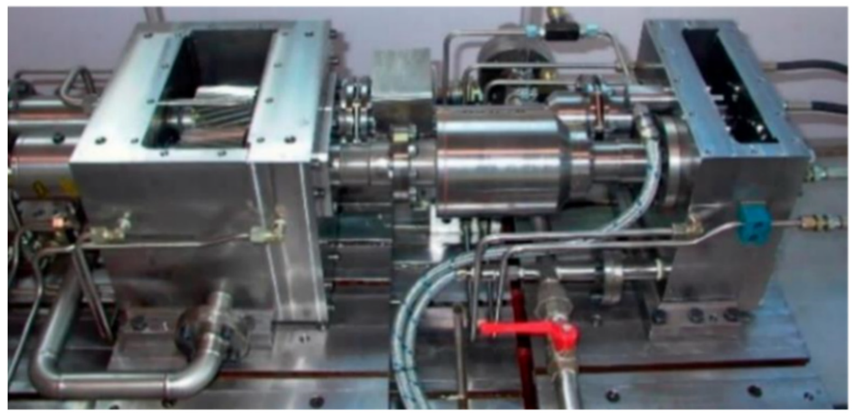
Figure 1. Test rig system layout used to perform the real tests.
Applsci 12 07814 g001
Figure 2. Three-dimensional model of the test rig displaying the main components of the system, including the helical and spur gear pairs (contact surfaces between the bodies) and the coupler (hydraulic loading mechanism).
Applsci 12 07814 g002
Figure 3. Numerical model of the test rig system considering the contact between the meshing surfaces of the gear teeth of the helical gear pair (right side) and the spur gear pair (left side), where the main analysis is performed for the healthy system and cases of damage.
Applsci 12 07814 g003
Figure 4. Elements and positions for the dynamic FEM simulations of the cases of damage. The axial reference axis was considered in three different positions (AD1, AD2, and AD3), representing the axial location of the damage, while each axial position location considered five different elements representing the severity of damage (ELEMs 1, 2, 3, 4, and 5).
Applsci 12 07814 g004
Figure 5. Deformed view of (a) medium and (b) severe damages of the first multi-class classification case.
Applsci 12 07814 g005
Figure 6. Deformed view of damages (a) 1 and (b) 2 of the second multi-class classification case.
Applsci 12 07814 g006
Figure 7. Deformed view of damages (a) 3 and (b) 4 of the second multi-class classification case.
Applsci 12 07814 g007
Figure 8. Simulation data organization for the first case (classification approach).
Applsci 12 07814 g008
Figure 9. Simulation data organization for the second case (first multi-class classification approach).
Applsci 12 07814 g009
Figure 10. Simulation data organization for the third case (second multi-class classification approach).
Applsci 12 07814 g010
Figure 11. Points representing each object location from the simulated model of the test bench (tangential shaft surface). The first step aimed at the extraction of the displacements from each point, while the second step aimed at the extraction of the vibrations after a double integration.
Applsci 12 07814 g011
Figure 12. Example of a Neural Network Pattern Recognition for damage presence (classification). W is the weight and b is the bias, which are the learnable parameters of the ANN model.
Applsci 12 07814 g012
Figure 13. Example of a Neural Network Pattern Recognition for damage severity (multi-class classification). W is the weight and b is the bias, which are the learnable parameters of the ANN model.
Applsci 12 07814 g013
Figure 14. Example of target file for a classification problem.
Applsci 12 07814 g014
Figure 15. Example of target file for a multi-class classification problem.
Applsci 12 07814 g015
Figure 16. Example of signals for the classification problem in the (a) time and (b) frequency domains. Both domains show comparisons of vibrational spectra on a bearing between a healthy transmission and a damaged one.
Applsci 12 07814 g016
Figure 17. Example of signals for the multi-class classification problems in the (a) time and (b) frequency domains. Both domains show comparisons of vibrational spectra on a bearing between a healthy transmission and cases of damage.
Applsci 12 07814 g017
Figure 18. The detection performances of the ANN for Test 1. The results provided responses for the training, validation, and test phases.
Applsci 12 07814 g018
Figure 19. Plots of the results for Test 1. The (a) validation performance, (b) error histogram, and (c) training state of the ANN provided responses for the training, validation, and test phases.
Applsci 12 07814 g019
Figure 20. The detection performances of the ANN for Test 2. The results provided responses for the training, validation, and test phases.
Applsci 12 07814 g020
Figure 21. Plots of the results for Test 2. The (a) validation performance, (b) error histogram, and (c) training state of the ANN provided responses for the training, validation, and test phases.
Applsci 12 07814 g021
Figure 22. The detection performances of the ANN for Test 3. The results provided responses for the training, validation, and test phases.
Applsci 12 07814 g022
Figure 23. Plots of the results for Test 3. The (a) validation performance, (b) error histogram, and (c) training state of the ANN provided responses for the training, validation, and test phases.
Applsci 12 07814 g023
Figure 24. The detection performances of the ANN for Test 4. The results provided responses for the training, validation, and test phases.
Applsci 12 07814 g024
Figure 25. Plots of the results for Test 4. The (a) validation performance, (b) error histogram, and (c) training state of the ANN provided responses for the training, validation, and test phases.
Applsci 12 07814 g025
Figure 26. The detection performances of the ANN for Test 5. The results provided responses for the training, validation, and test phases.
Applsci 12 07814 g026
Figure 27. Plots of the results for Test 5. The (a) validation performance, (b) error histogram, and (c) training state of the ANN provided responses for the training, validation, and test phases.
Applsci 12 07814 g027
Figure 28. The detection performances of the ANN for Test 6. The results provided responses for the training, validation, and test phases.
Applsci 12 07814 g028
Figure 29. Plots of the results for Test 6. The (a) validation performance, (b) error histogram, and (c) training state of the ANN provided responses for the training, validation, and test phases.
Applsci 12 07814 g029
Figure 30. The detection performances of the ANN for Test 7. The results provided responses for the training, validation, and test phases.
Applsci 12 07814 g030
Figure 31. Plots of the results for Test 7. The (a) validation performance, (b) error histogram, and (c) training state of the ANN provided responses for the training, validation, and test phases.
Applsci 12 07814 g031
Figure 32. The detection performances of the ANN for Test 8. The results provided responses for the training, validation, and test phases.
Applsci 12 07814 g032
Figure 33. Plots of the results for Test 8. The (a) validation performance, (b) error histogram, and (c) training state of the ANN provided responses for the training, validation, and test phases.
Applsci 12 07814 g033
Figure 34. The detection performances of the ANN for Test 9. The results provided responses for the training, validation, and test phases.
Applsci 12 07814 g034
Figure 35. Plots of the results for Test 9. The (a) validation performance, (b) error histogram, and (c) training state of the ANN provided responses for the training, validation, and test phases.
Applsci 12 07814 g035
Table 1. Test bench parameters.
ParametersSymbolStage 1 (Service Gearbox)Stage 2 (Test Gearbox)Units
Helical Gear 1Helical Gear 2Spur Gear 1Spur Gear 2
Center distance C d 91.591.5mm
Face width b 8014mm
N° of teeth z 34361718-
Normal module m n 2.55.0mm
Mass m 3.13.33.13.3 kg
Moment of inertia J 0.01220.01460.01220.0146 kg   m 2
Pitch circle diameter d p 0.08880.09410.08880.0941 m
Pressure angle α n 2020 deg
Helix angle β 120 deg
Contact ratio ε 1.05881.05881.05881.0588-
Young’s modulus E 200200GPa
Poisson’s ratio ν 0.30.3-
Table 2. Damage index.
Set of Simulations
Damage IndexAxial Dimension (AD) LongitudinalRadial Dimension (RD)
Nº ElementsClearance (0 mm)
Crack 11
Crack 22
Crack 33
Crack 44
Crack 55
Simulated SystemsDamages
1No crack-
2Pos 1-AD1Crack 1
3Pos 2-AD1Crack 2
4Pos 3-AD1Crack 3
5Pos 4-AD1Crack 4
6Pos 5-AD1Crack 5
7Pos 6-AD2Crack 1
8Pos 7-AD2Crack 2
9Pos 8-AD2Crack 3
10Pos 9-AD2Crack 4
11Pos 10-AD2Crack 5
12Pos 11-AD3Crack 1
13Pos 12-AD3Crack 2
14Pos 13-AD3Crack 3
15Pos 14-AD3Crack 4
16Pos 15-AD3Crack 5
Table 3. Important parameters from the “nprtool” interface.
Neural Pattern Recognition (nprtool)
ResultsSamplesCE%E
Training810.7944941.60494
Validation271.568951.85185
Testing271.586253.33333
Note 1. Important parameters from the “nprtool” interface. Minimizing Cross-Entropy (CE) results in good classification. Lower values are better. Zero means no error. Note 2. Percent Error (%E) indicates the fraction of samples that are misclassified. A value of 0 means no misclassifications; 100 indicates the maximum of misclassifications.
Table 4. Confusion Matrix Guide—Classification Method.
Confusion Matrix Guide—Classification Method
Total Number of Objects (n) = 360Predicted: No Damage (0)Predicted: Damage (1)Actual Objects (a)
Actual (0)TN = 175FP = 4a1 = TN + FP = 179a = a1 + a2 = n = 360
Actual (1)FN = 5TP = 176a2 = FN + TP = 181
Predicted Objects (p)p1 = TN + FN = 180p2 = FP + TP = 180
p = p1 + p2 = n = 360
Label 1
True Negative (TN)Predicted no damage: yes, and there is no damage.
True Positive (TP)Predicted damage: yes, and there is damage.
False Negative (FN)Predicted no damage: yes, and there is damage.
False Positive (FP)Predicted damage: yes, and there is no damage.
Label 2
Accuracy IndexWhat is the percentage of correct results for the classifier?
(TN + TP)/n = (175 + 176)/360 = 0.975 = 97.5%
Misclassification IndexWhat is the percentage of wrong results for it?
(FP + FN)/n = (4 + 5)/360 = 0.025 = 2.5%
True-Positive IndexWhen it is actually (1), what is the percentage of damage (1) prediction for it?
TP/a2 = 176/181 = 0.972 = 97.2%
False-Positive IndexWhen it is actually (0), what is the percentage of damage (1) prediction for it?
FP/a1 = 4/179 = 0.022 = 2.2%
True-Negative IndexWhen it is actually (0), what is the percentage of no damage (0) prediction for it?
TN/a1 = 175/179 = 0.978 = 97.8%
False-Negative IndexWhen it is actually (1), what is the percentage of no damage (0) prediction for it?
FN/a2 = 5/181 = 0.028 = 2.8%
Precision Index (0)When it predicts no damage (0), what is the percentage of correct results for it?
TN/p1 = 175/180 = 0.972 = 97.2%
No-Precision Index (0)When it predicts no damage (0), what is the percentage of wrong results for it?
FN/p1 = 5/180 = 0.028 = 2.8%
Precision Index (1)When it predicts damage (1), what is the percentage of correct results for it?
TP/p2 = 85/90 = 0.978 = 97.8%
No-Precision Index (1)When it predicts damage (1), what is the percentage of wrong results for it?
FP/p2 = 5/90 = 0.022 = 2.2%
Table 5. Confusion Matrix Guide—Multi-Class Classification Method.
Confusion Matrix Guide—Multi-Class Classification Method
Number of Objects (n) = 135Predicted: No Damage (1)Predicted: Medium Damage (2)Predicted: Severe Damage (3)Actual Objects (a)
Actual (1)TND11 = 42FMD12 = 0FSD13 = 3a1 = TND11 + FMD12 + FSD13 = 45a = a1 + a2 + a3 = n = 135
Actual (2)FND21 = 1TMD22 = 45FSD23 = 1a2 = FND21 + TMD22 + FSD23 = 47
Actual (3)FND31 = 2FMD32 = 0TSD33 = 41a3 = FND31 + FMD32 + TSD33 = 43
Predicted Objects (p)p1 = TND11 + FND21 + FND31 = 45p2 = FMD12 + TMD22 + FMD32 = 45p3 = FSD13 + FSD23 + TSD33 = 45
p = p1 + p2 + p3 = n = 135
Label 1
True No Damage (TND11)Predicted no damage: yes, and there is no damage.
False No Damage (FND21)Predicted no damage: yes, and there is damage.
False No Damage (FND31)Predicted no damage: yes, and there is damage.
False Medium Damage (FMD12)Predicted medium damage: yes, and there is no damage.
True Medium Damage (TMD22)Predicted medium damage: yes, and there is damage.
False Medium Damage (FMD32)Predicted medium damage: yes, and there is no damage.
False Severe Damage (FSD13)Predicted severe damage: yes, and there is no damage.
False Severe Damage (FSD23)Predicted severe damage: yes, and there is no damage.
True Severe Damage (TSD33)Predicted severe damage: yes, and there is damage.
Label 2
Accuracy IndexWhat is the percentage of correct results for the classifier?
(TND11 + TMD22 + TSD33)/n = (42 + 45 + 41)/135 = 0.948 = 94.8%
Misclassification IndexWhat is the percentage of wrong results for it?
(FND21 + FND31 + FMD12 + FMD32 + FSD13 + FSD23)/n = (1 + 2 + 0 + 0 + 3 + 1)/135 = 0.052 = 5.2%
True No Damage IndexWhen it is actually (1), what is the percentage of no damage (1) prediction for it?
TND11/a1 = 42/45 = 0.933 = 93.3%
False No Damage IndexWhen it is actually (1), what is the percentage of medium damage (2) and severe damage (3) predictions for it?
(FMD12 + FSD13)/a1 = (0 + 3)/45 = 0.067 = 6.7%
True Medium Damage IndexWhen it is actually (2), what is the percentage of medium damage (2) prediction for it?
TMD22/a2 = 45/47 = 0.957 = 95.7%
False Medium Damage IndexWhen it is actually (2), what is the percentage of no damage (1) and severe damage (3) predictions for it?
(FND21 + FSD23)/a2 = (1 + 1)/47 = 0.043 = 4.3%
True Severe Damage IndexWhen it is actually (3), what is the percentage of severe damage (3) prediction for it?
TSD33/a3 = 41/43 = 0.953 = 95.3%
False Severe Damage IndexWhen it is actually (3), what is the percentage of no damage (1) and medium damage (2) predictions for it?
(FND31 + FMD32)/a3 = (2 + 0)/43 = 0.047 = 4.7%
Precision Index (1)When it predicts no damage (1), what is the percentage of correct results for it?
TND11/p1 = 42/45 = 0.933 = 93.3%
No-Precision Index (1)When it predicts no damage (1), what is the percentage of wrong results for it?
(FND21 + FND31)/p1 = (1 + 2)/45 = 0.067 = 6.7%
Precision Index (2)When it predicts medium damage (2), what is the percentage of correct results for it?
TMD22/p2 = 45/45 = 1.000 = 100.0%
No-Precision Index (2)When it predicts medium damage (2), what is the percentage of wrong results for it?
(FMD12 + FMD32)/p2 = (0 + 0)/45 = 0.000 = 0.0%
Precision Index (3)When it predicts severe damage (3), what is the percentage of correct results for it?
TSD33/p3 = 41/45 = 0.911 = 91.1%
No-Precision Index (3)When it predicts severe damage (3), what is the percentage of wrong results for it?
(FSD13 + FSD23)/p3 = (3 + 1)/45 = 0.089 = 8.9%
Publisher’s Note: MDPI stays neutral with regard to jurisdictional claims in published maps and institutional affiliations.