Abstract
Traveling salesman, linear ordering, quadratic assignment, and flow shop scheduling are typical examples of permutation-based combinatorial optimization problems with real-life applications. These problems naturally represent solutions as an ordered permutation of objects. However, as the number of objects increases, finding optimal permutations is extremely difficult when using exact optimization methods. In those circumstances, approximate algorithms such as metaheuristics are a plausible way of finding acceptable solutions within a reasonable computational time. In this paper, we present a technique for clustering and discriminating ordered permutations with potential applications in developing neural network-guided metaheuristics to solve this class of problems. In this endeavor, we developed two different techniques to convert ordered permutations to binary-vectors and considered Adaptive Resonate Theory (ART) neural networks for clustering the resulting binary vectors. The proposed binary conversion techniques and two neural networks (ART-1 and Improved ART-1) are examined under various performance indicators. Numerical examples show that one of the binary conversion methods provides better results than the other, and Improved ART-1 is superior to ART-1. Additionally, we apply the proposed clustering and discriminating technique to develop a neural-network-guided Genetic Algorithm (GA) to solve a flow-shop scheduling problem. The investigation shows that the neural network-guided GA outperforms pure GA.
1. Introduction
In the last two decades, various approximate algorithms were introduced, focussing on their basic guidelines to quickly find feasible and suitable solutions to complex problems. These algorithms are commonly referred to as metaheuristic algorithms [1,2]. Among these algorithms, evolutionary algorithms (EAs), which include Genetic Algorithm (GA), Differential Evolution (DE), Evolutionary Strategy (ES), and Genetic Programming (GP), have been growing very quickly in terms of research developments and application areas [3]. GA has attracted the most researchers due to its various advantages, such as its ability to solve combinatorial hard problems with multiple solutions using a global search and its suitability for broader classes of problems [4,5].
These classes of algorithms produce a large amount of data during the search process. Unfortunately, these algorithms do not analyze the data generated during the search process. However, artificial intelligence, such as machine learning (ML), can help to analyze the generated data and provide helpful information from the search results, making EAs more intelligent and powerful. Luckily, the Artificial Intelligence (AI) research is flourishing at rocket speed in each sector of our daily life [6]. ML is a promising and significant research field in AI, which has been developing very rapidly and is used in various problems as a solo or an integrated part of a wider solution methodology [7]. Therefore, it is reasonable to assume that the enhancement of EAs (in terms of both solution quality and convergence speed) can be accomplished by using ML during the search process [3,8].
In the literature, different ML techniques have been used in various EAs. ANN is an ML technique that is widely used in the engineering, automotive, medicine, economics, aerospace, and energy sectors, and in many other fields [6,9,10]. ANN is adopted to limit the GA’s search space in some applications, such as silicon clustering and allocation problems [11,12]. Sivapathasekaran et al. [13] used GA and ANN to maximize biosurfactant production. The statistical experimental strategy was used to obtain the results, which was further used to link the ANN with GA. It was reported that the proposed hybrid system could boost production by nearly 70%. Palmes et al. [14] used a back mutation-based genetic neural network instead of backpropagation ANN. The proposed approach gave the network dynamics a good structure. This system helps to consider a wider range of populations with more flexibility and less restriction. Patra et al. [15] used ANN-based GA to design materials. Their study’s main aim was to give GA the ability to learn and speed up the evolutionary process. Deane [16] also used GA and augmented NN to solve the online advertisement scheduling issue. Moreover, Inthachot et al. [17] considered the combination of ANN and GA when evaluating the stock price trend in Thailand. Chen et al. [18] used the ART-1 network with tabu search optimization technique to solve the cell formation problems. The ART ANN was only used to find an initial solution. The use of machine-learning techniques as a mechanism to deal with initial solution generation has also been widely reported (see, for instance, [19,20,21,22]).
Burton and Vladimirova [23] proposed the use of an ARTMAP neural network as a fitness evaluator of GA. The authors showed that ART could be used to generate clusters depending on the vigilance value. Furthermore, Burton and Vladimirova [24] also proposed their ART as a fitness evaluator of GA for musical composition. The use of ML as a mechanism to evaluate the fitness of a solution was also reported in several other publications. A neural-network-embedded GA was proposed to solve a non-linear time–cost tradeoff problem for project scheduling in [25]. The ANN was used for the rapid estimation of the time–cost relationship. Other research articles that apply ML for fitness evaluation include [26,27,28,29,30].
In addition to the initialization of solution and fitness evaluation, ML applications to guide metaheuristics during the search process have been reported in the literature. The Q-learning-based selection of perturbation mechanism for a greedy metaheuristics algorithm to solve the scheduling problem was proposed in [31]. The purpose operator selection derived from the fact that individual operators may be particularly effective at certain stages of the search process, but perform poorly at others [32]. Some recent research using ML for operator selection in metaheuristics was published in [33,34,35].
Another variant of the use of ML is metaheuristics learnable evolution models (LEM), in which the lessons learned from previous generations are used to guide metaheuristics [36]. In these approaches, a machine learning algorithm seeks to extract information from the search space to either guide the metaheuristics to a more promising region (exploitation) or help the algorithm scape local optima (exploration). The LEM model for a general discrete optimization problem was developed in [37]. Its application in specific areas, such as the vehicle routing problem in [38], pickup and delivery optimization in [39,40], finned-tube evaporator in [41], and water-distribution system in [42], were illustrated. Readers interested in a comprehensive review of the various techniques used to integrate machine learning to assist metaheuristics are referred to [32].
In this paper, we developed a technique for clustering and discriminating ordered permutations with potential applications in the development of a neural-network-guided genetic algorithm to solve permutation-based optimization problems. This class of problems includes traveling salesman, linear ordering, quadratic assignment, and flow shop scheduling. In this effort, we developed two techniques to convert ordered permutations to binary vectors and considered Adaptive Resonate Theory (ART) neural networks for clustering the resulting binary vectors. The proposed binary conversion techniques and two neural networks (ART-1 and Improved ART-1) were examined under various performance indicators. Three performance indicators (misclassification, cluster homogeneity, and average distance) were introduced to empirically examine the proposed binary conversion methods. Numerical examples show that one of the binary conversion methods provides better results than the other, and Improved ART-1 is superior to ART-1. Later, a framework for a neural-network-guided GA was developed to solve permutation-based optimization problems by employing the proposed permutation-to-binary conversion method and ART-based neural network. Finally, a case study was conducted to solve a flexible flow shop scheduling problem. The results indicate that the Improved-ART-1 NN-guided GA with binary conversion method-1 performs better than pure GA. The work presented in this paper is an expansion of a conference proceeding by Tahsien and Defersha [43].
The remainder of this paper is organized as follows: Section 2 presents the basic concept of the ART neural network; Section 3 shows the proposed binary conversion methods; Section 4 illustrates the clustering ordered permutations under experimental data generation, performance criteria, and empirical analysis; a case study based on flow shop scheduling is investigated in Section 6; lastly, Section 7 presents the conclusions and future work.
2. Adaptive Resonance Theory Neural Network
A Neural Network (NN) is generally referred to as an Artificial Neural Network (ANN) inspired by biological nerve systems. An ANN consists of several interconnected neurons such as human brains, weights, and propagation function [44]. Among the various neural networks, Adaptive Resonance Theory (ART) is a fast learning technique, developed by Gali Carpenter and Stephen Grossberg in 1987 [45]. The ART neural network clarifies various brain and cognitive data types, where the ART adopts an unsupervised NN learning mechanism. The ART generally executes an algorithm to cluster the binary input vectors. Moreover, the ART is commonly used in face recognition, signature verification, mobile robot control, remote sensing, airplane design, autonomous adaptive robot control, target recognition, medical diagnosis, face recognition, land-cover classification, fitness evaluation, etc. [4,5]. Hence in this work, the research focused on ART-1 and Improved-ART-1 neural networks.
2.1. ART-1
ART-1 is a fast-learning technique that deals with binary input vectors for clustering purposes among various ART neural networks. Moreover, ART-1 can easily tackle the implementation of high-performance hardware. In addition, ART-1 exhibits a stable performance even during the learning stage by taking new inputs or information. Additionally, ART-1 can be described mathematically, which is suitable for design applications.
The ART-1 consists of two subsystems: attention and orientation. The attention subsystem includes two main layers of ART-1 architecture: the recognition layer and comparison layer with feed-forward and feed-backward features [46]. The attention subsystem is responsible for matching the input patterns with the stored patterns, and resonance is established if the pattern matches. The recognition layer, termed the F2 layer, a top-down layer, deals with the input vectors to compare the original vectors using a factor called vigilance. This vigilance is a measuring parameter to determine the distance between the input and the fired neuron’s clusters center in the recognition layer. The comparison layer, termed an F1 layer, is a bottom-up layer. This comparison layer deals with three types of input: (i) the input pattern X, i.e., , , … ; (ii) the gain input to each of the neuron (G1); (iii) the input from recognition layer as the feedback signal.
On the other hand, the orienting subsystem determines the mismatch between the top-down and bottom-up patterns in the recognition layers. There are an additional three units in the ART-1 architecture: Gain-1 and Gain-2 and Reset. The primary learning algorithms of ART-1 are as follows [46]:
- Step 1:
- The vigilance parameter, learning rate, and weights are initialized as follows:where, x is the number of input vector, L is a constant, are the bottom-up weights, i is the number of neurons, and j is the recognition layer’s neuron.
- Step 2:
- When an input vector is introduced in the ART neural network, the recognition layer begins the comparison and finds the maximum of all the neurons’ net output.
- Step 3:
- Run the vigilance test. A neuron (j) in the recognition layer passes the vigilance test only ifwhere is the vigilance threshold, is the net output of the recognition layer, and N is the total number of neurons.
- Step 4:
- If the vigilance test fails, then obscure the current winner and go to step 1 to find another winning neuron. Repeat the whole process until a winning neuron passes the vigilance test, and then go to step 5.
- Step 5:
- If no neuron passes the vigilance test, then create a new neuron to accommodate the new input pattern.
- Step 6:
- Adjust and update the feed-forward weights from the winning neuron to the inputs. The updated bottom-up and top-down weights can be obtained as follows:where is the the output of the first neuron in the comparison layer, is the top-down weights.
- Step 7:
- If there is no input vector, then stop; otherwise, go to Step 2.
2.2. Improved-ART-1
The basic form of ART-1 sometimes generates unsatisfactory results. The reasons for this include: (i) the order of the input vectors determines the overall results of ART-1 and the classification process; (ii) if more inputs are provided at the same time, then the stored pattern becomes scattered, i.e., stored input vectors become more sparse; (iii) it is difficult to identify the suitable vigilance parameters, since cell numbers increase with higher vigilance values during computation [47]. These limit ART-1 from being widely used in ordered permutation-based applications, such as permutation-based flow shop problems. As a result, Dagli and Huggahalli [48] proposed an Improved-ART-1 by changing a few things in the ART-1 algorithm. The changes are as follows:
- (i)
- Column and rows will be arranged in decreasing increments of 1 s.
- (ii)
- The prototype patterns are stored during the training period according to one of the following equations:
3. Proposed Permutation to Binary Conversion Methods
A binary conversion technique is required to convert ordered permutations to binary input vectors. The proposed binary conversion technique can be applied in the development of a neural-network-guided metaheuristic algorithm to solve problems where solutions are ordered permutations. Many problems have this feature, such as traveling salesman problems, flow shop scheduling, and single-row facility layout. Since we have considered the ART-1 neural network learning mechanism for our investigation, which requires binary input vectors for clustering, we have proposed and discussed novel binary conversion methods and introduced performance evaluators to analyze these conversion methods.
3.1. Conversion Method-1
The first binary conversion method is called the matrix method (M1) since the permutation is arranged in a matrix format. If we consider N numbers of distinct objects, then it generates a matrix of . In this matrix, the rows are indexed by the natural order of the objects and the columns are indexed by the order of the objects in the permutation. Then the cell that corresponds to a particular object is marked by 1. Then certain number of cells to the left and righ of that particular cell are also marked by 1. The number of cells to the left or right is termed as half-width (HW), which plays a significant role during conversion. If the half-width is too wide, then the outcome binary representation will not distinguish two permutaion with more or less order. However, if this width is considerably narrow, changing a bit in the sequence may generate nonidentical matrixes in such a way that similar permeations are considered very dissimilar. Hence, HW is an important parameter in method-1 conversion. Figure 1 illustrates an example of binary conversion method-1 considering 20 distinct objects. According to method-1, matrix is created and put 1s accordingly. Here, an HW of 3 (3 positions from the left and right) is examined. In this figure, the second row from the bottom represents the permutation of 20 objects, and the bottom row represents the location of these objects in the permeation. For instance, at location 10 is object 19. From this object, we move 19 rows upward, and the cell at row 19, column 10, is marked as 1. Then nearby cells, three steps to the left and three steps to the right, are also marked where the three is the value of HW. The complete binary vector representation of the permutation sequence is achieved by concatenating the matrix’s rows formed in Figure 1.
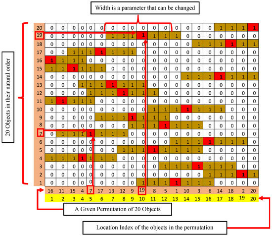
Figure 1.
Binary conversion method-1 (M1).
3.2. Conversion Method-2
The second binary conversion method (M2) is called the Base-2 method. This method first generates a new sequence based on the object’s location from the original permutation. The values of the elements of this new sequence are then converted into Base-2 numbers. Figure 2 shows the details of the Base-2 conversion methods, considering 20 objects. The bottom row is the location of the objects in the permutation. The second row (from bottom) is the permutation of the objects. The third row (from bottom) is the objects in their natural order. The fourth row (from bottom) is the locations of the objects sorted based on the natural order of the objects. These elements are then converted to base-2 numbers. The complete binary vector representation of the permutation considering the Base-2 number is achieved by concatenating the matrix’s columns, which are shown in Figure 2.
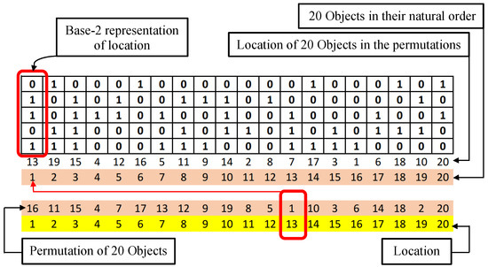
Figure 2.
Binary conversion method-2 (M2).
Here, it is important to note that binary conversion method-2 may have certain disadvantages compared to method-1. This is because there could be a drastic change in the binary encoding with a minor change in the permutations under binary conversion method-2, which is not the case in method-1. Figure 3 illustrates this limitation of conversion method-2 in detail.
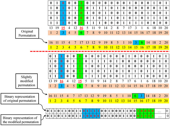
Figure 3.
Limitation of binary conversion method-2.
4. Clustering Ordered Permutations
In this section, experimental data generation, clustering performance criteria and detailed empirical investigations are discussed.
4.1. Experimental Data Generation
A controlled experimental data generation is required to analyze the ART-1 neural network and proposed binary conversion methods. Firstly, a specified number of ordered permutations are created randomly and named as seeds. Afterward, each seed is independently perturbed with a set degree of perturbation to generate many other permutations. In this way, the generation procedure helps to predict how many clusters are likely to exist in the randomly generated data. This is because the number of clusters will generally equal the number of seeds used to create the data.
4.2. Clustering Performance Criteria
This work introduced three clustering performance criteria, i.e., misclassification, homogeneity, and average distance, to evaluate the proposed binary conversation techniques and the neural networks used to cluster the randomly generated data.
4.2.1. Misclassification
Once clusters are identified, their centers are determined. Then, if a member of a cluster is closer to the centroid of another cluster to which it does not belong, it is said to be misclassified. Hence, misclassification plays a significant role in this investigation. For example, consider a cluster i, which contains number of permutations, and each permutation is defined as . Then, the cartesian coordinate of each permutation is represented as . Here, (, where N is the total number of objects) indicates the location of an object (n) in the permutation (p). Now, the cartesian coordinate of the centroid of cluster i along the nth axis can be calculated using Equation (7), as follows:
The centroid of cluster i is defined as . The distance () between any permutation p and a cluster centroid can be calculated as shown in Equation (8)
Assuming permutation p belongs to cluster i, if distance is greater than the distance of this permutation from at least one other cluster , then the permeation is termed to be misclassified. In this way, the total number of misclassified permutations in a given cluster can be computed.
4.2.2. Homogeneity
In defining homogeneity, we first define a new term “dominating seed” of a cluster as the seed from which most of the members of the cluster originate. Homogeneity is then defined as the ratio (percentage) of the number of members from the dominating seed to that of the total number of members of the cluster. A cluster is considered a better cluster if its homogeneity is higher than the other clusters.
4.2.3. Average Distance
Average distance is the third indicator of cluster quality, which is used to examine the performance of the proposed binary conversion methods for the ART-1 neural network. The ratio of the sum of the members’ distances from the centroid of their cluster to the total number of the members in the cluster is called the average distance. The smaller the average distance, the better (or the denser) the identified cluster.
4.3. Empirical Investigations
A comprehensive empirical investigation of the proposed binary conversion methods was performed, considering the ART-1 and Improved-ART-1 algorithms. The two binary conversion techniques are compared in the following subsections based on misclassification, homogeneity, and average distance. In this investigation, the number of seeds is 5, the number of solutions per seed is 500, the half-width is 3, the vigilance value is 0.5, and the number of objects is 40. Since the analysis provides slightly different solutions during each run, a total of 10 solutions was considered, and then the average of these ten solutions was taken. Table 1 presents a comparative study between binary conversion method-1 and method-2, adopting the ART-1 and Improved-ART-1 neural networks. The initial result indicates that the binary conversion method-1 (M1) outperforms method-2 using ART-1 and Improved-ART-1 in terms of all the clustering performance criteria (i.e., less misclassification, high homogeneity, and shorter average distance).

Table 1.
Performance analysis between binary conversion method-1 and method-2 considering ART-1 and Improved-ART-1 algorithms.
The previous analysis shows that the binary conversion method-1 provides satisfactory results. Now, the investigation is further extended to different problem sizes considering 10, 20, 30 and 40 objects, where the other parameters mentioned at the beginning of this section are kept constant. Table 2 shows the performance of binary conversion method-1 on both ART-1 and Improved-ART-1 neural networks, considering four different problem sizes. The results indicate that method-1 performs better than method-2, providing less misclassification, higher homogeneity, and a shorter average distance.

Table 2.
Comparison between binary conversion method-1 and method-2 for four different problem sizes considering ART-1 and Improved-ART-1. Here, M = misclassification, H = homogeneity, A.D. = Average Distance.
Figure 4 presents a comparative study between ART-1 and Improved-ART-1, in terms of misclassification, homogeneity, and average distance using binary conversion M1, since M1 outperforms compared to M2. It is seen that the number of ART-1 misclassifications is nearly 99% higher than when using Improved ART-1. Therefore, Improved-ART-1 with M1 leads to better-quality solutions than ART-1.
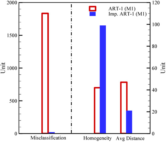
Figure 4.
Comparative study between Improved-ART-1 and ART-1 considering M-1.
Furthermore, a projection between the expected cluster numbers and the actual cluster generated by both neural networks using binary conversion method-1 is illustrated in Figure 5. It is reported that the Improved-ART-1 with method-1 matches and follows the trend of the anticipated number of clusters with an increment in seed number until 6, where the vigilance value is 0.5, degree of perturbation is 4, half-width is 3, and the number of solutions per seed is 500. However, the ART-1 neural network does not match the anticipated number of clusters, generating a higher cluster number than expected. Therefore, this analysis is another good indicator that Improved-ART-1 using the proposed binary conversion method-1 provides a better result than ART-1.
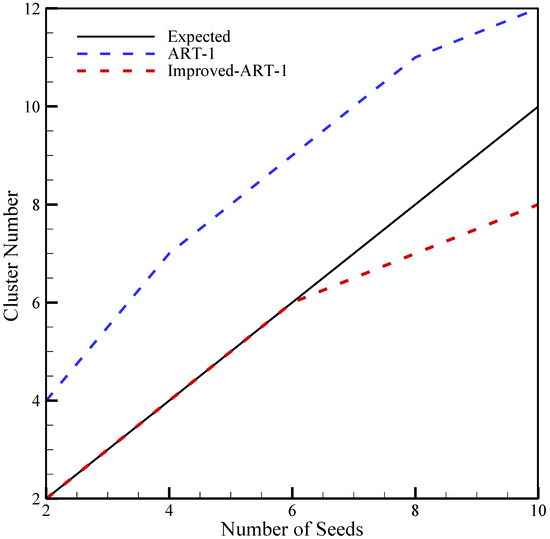
Figure 5.
Comparative study between ART-1 and Improved-ART-1 with M1 as a function of number of seeds where the vigilance value is 0.5.
5. Proposed Architecture ANN Guided GA
In this research work, an architecture of Improved-ART-1 neural network guided GA has been proposed. Since binary conversion method-1 had a better performance than method-2, method-1 was considered in the ART neural network’s proposed architecture. A detailed schematic diagram of the proposed ANN-guided GA is depicted in Figure 6. The three main parts of this architecture are GA, Improved-ART-1, and solution warehouse and cluster management (SWCM). A series of solutions, where each solution is ordered permutation, is evolved by GA in this SWCM system. The generated order permutation is then sent to the Improved-ART-1. In the ART, binary conversion method-1 occurs to convert ordered permutations into binary input vectors for clustering. Then, each solution is given a cluster-ID by the Improved-ART-1 neural network.
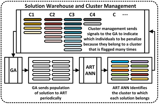
Figure 6.
Architecture of the Improved-ART-1 neural network-guided GA.
Once cluster ID is defined, each solution is sent to the SWCM unit. SWCM then sends each individual to its respective cluster and dynamically sorts the individuals within a cluster in such a way that the top position of the clusters carries the fitter individual. It is important to note that SWCM is a double-linked list that includes cluster iterator and insertion techniques. All this sorting within a cluster is automatically accomplished in the SWCM module, with less computational effort. It is also worth mentioning that SWCM stores unique solutions. The SWCM module puts a flag on a cluster if a large percentage of the incoming population is stored in that cluster. If a cluster is flagged more than a specified number of times, then the SWCM module sends a message to the GA. Then, the GA penalizes the individual from the flagged cluster. A randomly generated new individual solution then replaces the flagged cluster’s individual. When all the clusters are flagged, and there is no new cluster generation, the SWCM will reset the flag counter, and this process will continue until another reset is required. The proposed architecture helps GA to avoid stagnating in a specific search region.
6. Flow Shop Scheduling—A Case Study
Flow shop is a unidirectional model where each given job is processed in a set of stages arranged in order. In a classical flow shop scheduling problem (FSP), each stage has only one machine, and each job is processed in sequence without skipping a stage. Although it is the simplest form of a multi-stage manufacturing system, the classical flow shop with sequence-dependent setup time is a typical NP-hard problem where it is difficult to find the global optima. The other variant and the more complex form of flow shop scheduling, where there are parallel machines on at least one stage, and a job may skip certain stages, is known as a flexible flow shop problem (FFSP) [49]. FFSP is widely considered in the electronics, chemical, and automobile industries [49]. In this paper, we consider FFSP with sequence-dependent setup times when comparing the pure and the ANN-guided genetic algorithms.
6.1. Assumption and Notations
In this section, we present the assumptions, problems description, and notations of the FFSP that appeared in [50,51], in which a pure genetic algorithm was used to solve the problem.
6.1.1. Problem Description
Consider a manufacturing environment based on a flexible flow shop, where several consecutive production stages are used to process several jobs. It is assumed that each stage has a certain number of parallel machines. The parallel machines in each stage are assumed to be dissimilar. Each job has a specified number of units (called batch size). The jobs are processed in the order of the stages and batch of certain products may skip some stages. At any given stage, a job can be assigned to exactly one machine that is eligible to process that particular job. For each job, there is a sequence-dependent setup time on each eligible machine, and this setup may be anticipatory or non-anticipatory at different stages. Anticipatory setup can be perfumed before the job arrives at the stage if the assigned machine is free, whereas, in non-anticipatory setup, the job must arrive at the stage for the setup to begin. The problem is to determine the assignment and processing sequence of these jobs on each machine in each stage. The objective function is to minimize the completion time of the last sublot to be processed in the system.
6.1.2. Notations
The notations presented in this section were adopted from [50], where a pure genetic algorithm was used to solve the problem with lot streaming. The notation related to lot streaming was removed as the considered FJSP has no lot streaming. Lot streaming was removed since only ordered permutations were optimized. These notations are explained as follows:
| Indexes and Input Data | |
| I | Total number of stages where the stages are indexed by i or ; |
| Mi | Total number of machines in stage i where the machines are denoted by m or ; |
| N | Total number of jobs where the jobs are represented by n or ; |
| Pn | A set of pairs of stages for job n, i.e., the processing of job n in stage l is followed by its processing in stage i; |
| Tn,m,i | Total processing time for one unit of job n on machine m in stage i; |
| Qn | Batch size of job n; |
| Rm,i | Number of maximum production runs of machine m in stage i where the production runs are indexed by r or ; |
| Sm,i,n,p | Setup time on machine m in stage i for processing job n following the processing of job p on this machine; if , the setup may be called minor setup; |
| An,i | Binary data equal 1 if setup of job n in stage i is attached (non-anticipatory), or 0 if this setup is detached setup (anticipatory); |
| Bn,i | Binary data equal 1 if job n needs processing in stage i; otherwise, 0; |
| Dn,m,i | Binary data equal 1 if job n can be processed on machine m in stage i, otherwise 0; ; |
| Fm,i | The release date of machine m in stage i; |
| Ω | Large positive number. |
| Variables | |
| Continuous Variables: | |
| cn,i | Completion time of the job n from stage i; |
| Completion time of the rth run of machine m in stage i. | |
| Binary Variables: | |
| xr,m,i,n | Binary variable that takes the value 1 if the rth run on machine m in stage i is for the job n, 0 otherwise; |
| zr,m,i | A binary variable that equals 1 if the rth potential run of machine m in stage i has been assigned a job to process, 0 otherwise; |
| cmax | Makespan of the schedule. |
Given the above notations, a mixed-integer linear programming can be used to formalize the scheduling problem addressed in this paper. However, we used a solution representation of a genetic algorithm and the accompanying decoding procedure as a way to formalize the problem. The following section provides details of the genetic algorithm that is commonly used to solve flow shop scheduling. This algorithm is used as the main component of the ANN-Guided GA framework proposed in Section 5.
6.2. Components of Pure GA
In this section, we adapted the pure GA algorithm for FFSP problems from [50] to determine the optimal or near-optimal solutions. The main components of the pure genetic algorithm are solution representation, fitness evaluation, and genetic operator operators. These components are adapted to a situation where lot streaming is not addressed.
6.2.1. Solution Representation
Solution representation is critical component of any genetic algorithm, as the GA’s success and failure is mainly dependent on this [52]. Holland [53] stated that it is necessary to design the solution encoding correctly to successfully implement the GA. Permutation-based encoding is commonly used to solve flexible flow shop scheduling problems where the actual assignment and sequencing is determined by the accompanying decoding procedure. Figure 7 presents the GA’s solution representation, where we assume ten jobs in a randomly generated permutation (i.e., 3, 4, 1, 2, 9, 10, 6, 8, 7, 5). Each chromosome shows a permutation of N jobs, where N is the total number of jobs. In this chromosome, is the gene at the sth location, and is a numeric value equal to the indices of the job at that location. For example, in Figure 7, when equals 1, then it represents job 3, whereas represents job 4, and so on.

Figure 7.
Solution representation.
6.2.2. Fitness Evaluation
Once a solution representation is developed, developing the decoding procedure is vital to determine the fitness (makespan) of the corresponding schedule. The decoding is accomplished by a specific rule for assigning and sequencing the jobs guided by the permutation of the job in the chromosome under evaluation. In this paper, we considered an assignment rule and sequencing rule adopted from [50,54] by adjusting for a situation when lot streaming is not considred. The considered assignment rule takes care of: (i) the attached and detached setup time, (ii) release date of machines, (iii) the possibility of some jobs skipping some stages. If we consider job n, which is allocated for a machine m in stage i, then the completion time is calculated for one of the following cases:
- Case 1:
- If job n is considered the first job to be assigned to machine m, and stage i is the first stage for this job n; then, becomes .
- Case 2:
- If job p is the last job assigned to machine m and i is the first stage to be visited for job n, then becomes .
- Case 3:
- If job n is the first job to be assigned to machine m and this job n has to visit stage l before visiting stage i, then becomes .
- Case 4:
- If job p is the last job to be assigned to machine m, and job n has to visit stage l before visiting stage i, then becomes .
Assignment Rule
In the assignment rule, we consider sequence-dependent setup time, the processing times of different units on parallel machines, machine release date, and machine eligibility to calculate each job’s completion time in , visiting all the stages. Weadopted the assignment rule from the work presented in [54]. The basic steps are as follows:
- Step 1:
- Decode the sizes of each job for the considered chromosome and obtain the permutation from the chromosome (as shown in Figure 7). Initialize and .
- Step 2:
- Set .
- Step 3:
- If , go to Step 4; otherwise, go to Step 7.
- Step 4:
- If , go to Step 5; otherwise, go to Step 6.
- Step 5:
- Assign job n to one of the available machines m in stage i, where it will be completed at the earliest completion time .
- Step 6:
- If , set and go to Step 4; otherwise, go to Step 7.
- Step 7:
- If , set and go to Step 2; otherwise, go to Step 8.
- Step 8:
- Calculate . Here, defines the smallest makespan/completion time of all jobs processed in the system of considered chromosome.
6.2.3. Genetic Operators
Once we have each chromosome’s fitness value, the next step is to choose the best fitness value. GA operators develop a more promising solution from the initial population to replace the less promising solution, which is an important GA stage. Typically, three operators—selection, crossover, and mutation operators—participate in this process.
Selection Operator
The selection operator is the first operator used for reproduction, which means that this operator selects the chromosome that will participate in the next iteration in GA. Many selection operators are used in GA. Altenberg [55] stated that the selection operator’s primary objective is to determine the best fitness solution string that will reproduce a new solution string with enhanced fitness. The selection operator first participates in GA’s operation before crossover and mutation. In this work, we considered k-way tournament section operators. The individual k is chosen randomly in the k-way tournament, and the one with the highest fitness value becomes the winner and moves to the next generation. This process continues until the number of chosen individuals is equal to the size of the population, where, before each tounamet, the k individuates in the previous tournament before returning to the old population.
Crossover Operator
Once the selection is completed and new papulation is constituted, the chromosomes are randomly paired, and the crossover operator is applied with a certain probability. A crossover operator is used for each new pair of chromosomes to mix the information, in the hope of creating new children with a higher fitness value [50,55]. Different crossover operators are considered in the literature [56]. In this work, we adopted the single-point crossover (SPC). Figure 8 presents SPC, where the exchange took place on the left-hand side. The crossover operation was accomplished in the following manner:
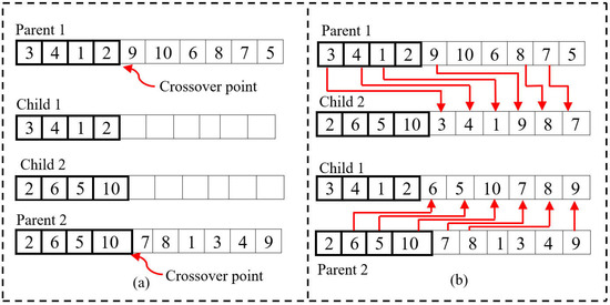
Figure 8.
Illustration of single point crossover: (a) Step-1, and (b) Step 2.
- Step 1:
- Firstly, the crossover point is arbitrarily chosen from each parent. Then, all genes from the left-hand side of both parents’ crossover points are copied to generate two children. Additionally, the genes from the right side of the crossover point will be removed in the new child (see Figure 8a).
- Step 2:
- The children are then interchanged between the parents, i.e., child 1 goes to parent 2, and child 2 comes to parent 1. At last, the missing jobs are placed in the relative order of the other parent (as shown in Figure 8b).
Mutation Operator
The mutation operator is another genetic operator that is deployed to the newly formed child after completing the crossover operation. It is also known as a perturbation operator. The mutation operator slightly changes the new child’s chromosomes in the hope of achieving a better result. Many mutation operators are used in GA, such as swap mutation, shift mutation, flip mutation, bit string mutation, scramble mutation, inversion mutation, Random Operation Assignment Mutation (ROAM), Intelligent Operations Assignment Mutation (IOAM), and Operations Sequence Shift Mutation (OSSM) [56]. In our work, we considered swap and shift mutation operators. In swap mutation, two genes are randomly selected, and their positions are exchanged. In shift mutation, a gene is randomly selected and moved to a randomly selected position.
6.3. Comparative Study: Pure GA vs. Improved-ART-1-Guided GA
This section presents a comparative study between the proposed algorithm Improved-ART-1 neural network guide using binary conversion method-1 and pure GA, considering both small and large problems.
6.3.1. Small Prototype Problem
Initially, a small prototype example of FFSP is considered for the MILP model. This prototype problem consists of eight jobs (n) that need to be processed in a total of four stages (i) using a maximum of two machines (m) in each stage. For instance, Table 3, Table 4 and Table 5 show the details of the small problem considered for FFSP. Table 3 shows that each stage is assigned two parallel machines, i.e., the work assignment can be carried out using one of the machines, depending on the calculated optimum processing time. We have also considered the machine release date in the proposed prototype problem. Machine release date is important in the production environment [51], since the available machine’s selection can be influenced by the release date.

Table 3.
A small example of case study consists of two machines and four stages.

Table 4.
The case study includes eight jobs with different batch sizes and processing times for each eligible machine.

Table 5.
Setup time for each eligible machine for each job.
Table 4 illustrates the processing time required by the machines, where a total of eight jobs were considered with various batch sizes that need to be completed at different stages. For example, job 1 (n) is completed in three stages (i.e., stage 1, 2, 4, and skipped stage 3), which involves three operations (o) considering a batch size () of 20. Here, indicates the machine’s state as a setup property. If is 1, then this setup is called attached or non-anticipatory. It also indicates that the machine setup will be determined once the job arrives at the machine. On the other hand, when is 0, it is called detached or anticipatory, which indicates that the machine’s setup must be completed before it arrives at the job on the machine. In the proposed case study, we considered both attached and detached setup conditions. The data for each eligible machine’s sequence-dependent setup time for different jobs at various stages are presented in Table 5.
6.3.2. Typical Solution for Small Problem
A typical solution to the proposed prototype problem is illustrated in Figure 9. The first row (numbered as 1, 2, …, 8) indicates the location of the chromosome gene. The solution encoding in Figure 9 will be decoded using the decoding procedure described earlier. The FFSP completion time will also be calculated based on the fitness evaluation rules explained in the previous section.

Figure 9.
A typical solution representation for FFSP.
An example of the GA decoding procedure for the solution representation is presented in Table 6. Table 3, Table 4 and Table 5 are considered for this partial decoding procedure. The GA decoding procedure details, including four cases (from Case 1 to Case 4) are described earlier. In the end, the total completion time of each job at four different stages, completed by each machine, can be calculated until all the jobs are assigned and processed. Figure 10 illustrates a pictorial presentation of the Gantt chart of the schedule corresponding to the solution presented in Figure 9. The Gantt chart indicates the features of the stated prototype problem, which requires a maximum makespan of 1835 min. Moreover, other attributes include the setup time for each machine in each stage, the lag time for each machine to go for production, and the overlapping issue in two consecutive stages due to the detached setup from the Gantt chart. For example, there are some jobs where is 0, which indicates that the setup time of that particular job in that stage can be started earlier, if possible, before the completion of the corresponding job from the previous stage. According to this, the setup time of job on machine and job on machine at stage , job and job at stage on machine and machine respectively, and job on machine and job on machine at stage were started earlier.

Table 6.
A partial decoding steps of GA for the solution representation in Figure 9. This decoding process will continue until all the jobs are assigned at each stage.
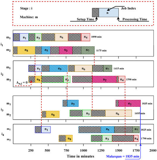
Figure 10.
Gantt chart of the scheduling for small prototype problem based on the decoding process stated in Table 6.
6.3.3. Performance Analysis When Solving Large Problems
Here, we examined the algorithm’s performance in a small-size problem. However, the previous analysis is insufficient since the problem size is small and cannot picture the real-world scenario and complexity. Therefore, we will compare pure GA and our proposed algorithm Improved-ART-1 neural-network-guided GA considering binary conversion method-1 for large-size problems. In this regard, six large problems were considered for this comparative study. These problems were generated and solved using the first 20 trials considering Pure GA with and without ANN intervention. Table 7 presents the general features of large problems with a considered number of jobs, number of stages, and minimum number of parallel machines, and the maximum number of batch sizes for each problem.

Table 7.
Features of considered large size problems.
We present six large problems in which we adopted our proposed binary conversion method-1 using Improved-ART-1 neural-network-guided GA and pure GA to solve FFSP. The problem lies in determining an effective sequence for the jobs at the first stage, so that all the jobs can be completed within a minimal amount of time (makespan). Each ordered sequence can be assigned a measure of goodness, which is makespan. Twenty trials were performed during the experiment by changing the seed to generate multiple solutions. Most of the trials show that the Improved-ART-1 guided GA provides better solutions with a lower makespan compared to pure GA (see Figure 11). It is clearly noticeable from the analysis of the six problems mentioned in Table 7 that ANN-guided GA not only converges quickly but also comes up with a better result (lower makespan) compared to pure GA.
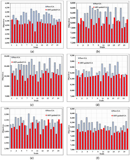
Figure 11.
Comparison between GA and ANN-guided GA for problems 1 to 6 detailed in Table 7. (a) Problem-1. (b) Problem-2. (c) Problem-1. (d) Problem-2. (e) Problem-1. (f) Problem-2.
One of the limitations of pure GA is that GA explores only specific clusters. This limits the searching process, which indicates GA’s exploitation, because regions that were previously explored by GA prevent the searching option blind from exploring other clusters. According to the proposed algorithm, ANN-guided GA architecture combines GA, ART, and SWCM, where SWCM helps GA to avoid being stuck in a specific search region. Thus, the intervention promotes exploration of the solution space so that other clusters find the optimal solution. Therefore, the results show that ANN-guided GA has an improved exploration ability compard to pure GA and can find an optimal solution by searching almost all clusters. The investigation of the assumed six different problem sizes provides further insight into the analysis, from which we can see that pure GA has been stuck in one region of the search space. GA without ANN is exploited in a particular cluster. Moreover, it can be said that GA is trapped in some regions: it is not clear that the result provided by GA is actually the optimal one, and it is still possible to obtain a better result from other clusters that have not been explored to date (as shown in Figure 12a,c,e). However, ANN intervention helps GA to explore almost all the clusters in the search space (see in Figure 12b,d,f).
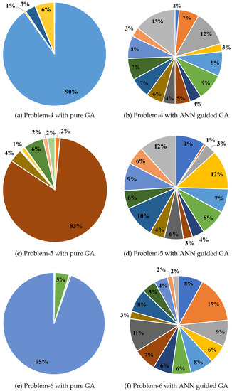
Figure 12.
Allocation of population with and without ANN intervention. (a,c,e) are the results of pure GA and (b,d,f) are for ANN-guided GA, considering problems 4, 5, and 6, respectively, as mentioned in Table 7; the legends represent the cluster id.
7. Conclusions and Future Research
In this work, we presented a technique to discriminate and cluster ordered permutation using ART-1 and Improved-ART-1 neural network-guided GA. In this process, two binary conversion techniques were introduced to convert ordered permutations to binary input vectors to use in ART-1 algorithms. The proposed binary conversion methods’ performance, considering ART-1 and Improved-ART-1, was evaluated under three performance indicators: misclassification, cluster homogeneity, and average distance. Additionally, the empirical study was extended by varying the problem sizes. The investigation shows that the Improved-ART-1 neural network with the proposed binary conversion method-1 provides better results than ART-1 in every scenario.
In addition, the detailed architecture of the proposed Improved-ART-1 guided GA was illustrated. A case study considering the flow shop scheduling problem was examined for small and large prototype problems based on the ANN-guided GA architecture. The empirical results show that the intervention of GA by ART-1 and SWCM prevents the algorithm from stagnating in a given region of the search space. Hence, the intervention promotes exploration of the solution space so that other clusters find the optimal solution. The Improved ART-1-guided GA has a better exploration ability than pure GA and can find an optimal solution by searching almost all the clusters. In addition, the performance result proves the competence of our proposed binary conversion method-1 with Improved-ART-1 neural-network-guided GA for any permutation-based combinational optimization with real-life applications.
The Improved-ART-1 in the proposed ANN-guided GA architecture only deals with binary input vectors, which be applied to any problems in which the solutions are not ordered permutations. Since we considered a flow shop scheduling problem for our case study, future work could focus on applying the proposed binary conversion method-1-based Improved-ART-1-guided GA to other scheduling problems, such as job shop and open shop, whose solution may not be a pure ordered permutation. Moreover, the other metaheuristics algorithms, such as tabu search, ant colony, swarm intelligence, simulated annealing, etc., which are guided by ART-1, can be considered for scheduling problems and compared to our current technique. Our developed ANN-guided GA application area should not be limited to manufacturing scheduling problems; it can be considered for other application fields, such as image recognition, pattern recognition, mobile robot control, signature verification, medical diagnosis, etc.
Author Contributions
S.M.T.: Methodology, Investigation, Validation, Formal analysis, Writing—Original Draft, Data Curation; F.M.D.: Conceptualization, Methodology, Formal analysis, Software, Validation, Visualization, Writing—Review and Editing, Supervision. All authors have read and agreed to the published version of the manuscript.
Funding
This research was funded by the Discovery Grant from NSERC, the Natural Science and Engineering Research Counsel of Canada (https://www.nserc-crsng.gc.ca/index_eng.asp), accessed on 1 January 2020.
Data Availability Statement
Available upon request made to the corresponding author.
Acknowledgments
We would like to thank all three anonymous reviewers for their suggestions that helped us to improve the paper.
Conflicts of Interest
The authors declare no conflict of interest.
References
- Mahadevan, E.G. Ammonium Nitrate Explosives for Civil Applications: Slurries, Emulsions and Ammonium Nitrate Fuel Oils; John Wiley & Sons: Hoboken, NJ, USA, 2009. [Google Scholar] [CrossRef]
- Talbi, E.G. Machine Learning into Metaheuristics: A Survey and Taxonomy; Technical Report 6. ACM Comput. Surv. 2021, 54, 1–32. [Google Scholar] [CrossRef]
- Zhang, J.; Zhang, Z.H.; Lin, Y.; Chen, N.; Gong, Y.J.; Zhong, J.H.; Chung, H.S.; Li, Y.; Shi, Y.H. Evolutionary computation meets machine learning: A survey. IEEE Comput. Intell. Mag. 2011, 6, 68–75. [Google Scholar] [CrossRef]
- Mehta, A. A Comprehensive Guide to Neural Networks. Digitalvidya 2019, 2. [Google Scholar]
- Grossberg, S. Adaptive Resonance Theory: How a brain learns to consciously attend, learn, and recognize a changing world. Neural Netw. 2013, 37, 1–47. [Google Scholar] [CrossRef]
- Yang, C.; Ge, S.S.; Xiang, C.; Chai, T.; Lee, T.H. Output feedback NN control for two classes of discrete-time systems with unknown control directions in a unified approach. IEEE Trans. Neural Netw. 2008, 19, 1873–1886. [Google Scholar] [CrossRef] [PubMed]
- Mjolsness, E.; DeCoste, D. Machine learning for science: State of the art and future prospects. Science 2001, 293, 2051–2055. [Google Scholar] [CrossRef]
- Zurada, J.M.; Mazurowski, M.A.; Ragade, R.; Abdullin, A.; Wojtudiak, J.; Gentle, J. Building virtual community in computational intelligence and machine learning. IEEE Comput. Intell. Mag. 2009, 4, 43–54. [Google Scholar] [CrossRef]
- Kumar, R.; Aggarwal, R.K.; Sharma, J.D. Energy analysis of a building using artificial neural network: A review. Energy Build. 2013, 65, 352–358. [Google Scholar] [CrossRef]
- Alippi, C.; De Russis, C.; Piuri, V. A neural-network based control solution to air-fuel ratio control for automotive fuel-injection systems. IEEE Trans. Syst. Man Cybern. Part C Appl. Rev. 2003, 33, 259–268. [Google Scholar] [CrossRef]
- Marim, L.R.; Lemes, M.R.; Dal Pino, A. Neural-network-assisted genetic algorithm applied to silicon clusters. Phys. Rev. A-At. Mol. Opt. Phys. 2003, 67, 8. [Google Scholar] [CrossRef]
- Lee, C.; Gen, M.; Kuo, W. Reliability optimization design using a hybridized genetic algorithm with a neural-network technique. IEICE Trans. Fundam. Electron. Commun. Comput. Sci. 2001, E84-A, 627–637. [Google Scholar]
- Sivapathasekaran, C.; Mukherjee, S.; Ray, A.; Gupta, A.; Sen, R. Artificial neural network modeling and genetic algorithm based medium optimization for the improved production of marine biosurfactant. Bioresour. Technol. 2010, 101, 2884–2887. [Google Scholar] [CrossRef]
- Palmes, P.P.; Hayasaka, T.; Usui, S. Mutation-based genetic neural network. IEEE Trans. Neural Netw. 2005, 16, 587–600. [Google Scholar] [CrossRef]
- Patra, T.K.; Meenakshisundaram, V.; Hung, J.H.; Simmons, D.S. Neural-Network-Biased Genetic Algorithms for Materials Design: Evolutionary Algorithms That Learn. ACS Comb. Sci. 2017, 19, 96–107. [Google Scholar] [CrossRef]
- Deane, J. Hybrid genetic algorithm and augmented neural network application for solving the online advertisement scheduling problem with contextual targeting. Expert Syst. Appl. 2012, 39, 5168–5177. [Google Scholar] [CrossRef]
- Inthachot, M.; Boonjing, V.; Intakosum, S. Artificial Neural Network and Genetic Algorithm Hybrid Intelligence for Predicting Thai Stock Price Index Trend. Comput. Intell. Neurosci. 2016, 2016. [Google Scholar] [CrossRef] [PubMed]
- Chen, M.L.; Wu, C.M.; Chen, C.L. An integrated approach of art1 and tabu search to solve cell formation problems. J. Chin. Inst. Ind. Eng. 2002, 19, 62–74. [Google Scholar] [CrossRef][Green Version]
- Cheng, C.Y.; Pourhejazy, P.; Ying, K.C.; Lin, C.F. Unsupervised Learning-based Artificial Bee Colony for minimizing non-value-adding operations. Appl. Soft Comput. 2021, 105, 107280. [Google Scholar] [CrossRef]
- Ali, I.M.; Essam, D.; Kasmarik, K. A novel design of differential evolution for solving discrete traveling salesman problems. Swarm Evol. Comput. 2020, 52, 100607. [Google Scholar] [CrossRef]
- Nasiri, M.M.; Salesi, S.; Rahbari, A.; Salmanzadeh Meydani, N.; Abdollai, M. A data mining approach for population-based methods to solve the JSSP. Soft Comput. 2019, 23, 11107–11122. [Google Scholar] [CrossRef]
- Min, J.N.; Jin, C.; Lu, L.J. Maximum-minimum distance clustering method for split-delivery vehicle-routing problem: Case studies and performance comparisons. Adv. Prod. Eng. Manag. 2019, 14, 125–135. [Google Scholar] [CrossRef]
- Burton, A.R.; Vladimirova, T. Utilisation of an adaptive resonance theory neural network as a genetic algorithm fitness evaluator. In Proceedings of the IEEE International Symposium on Information Theory-Proceedings, Ulm, Germany, 29 June–4 July 1997; p. 209. [Google Scholar] [CrossRef]
- Burton, A.R.; Vladimirova, T. Genetic Algorithm Utilising Neural Network Fitness Evaluation for Musical Composition. Artif. Neural Nets Genet. Algorithms 1998, 219–223. [Google Scholar] [CrossRef]
- Pathak, B.K.; Srivastava, S.; Srivastava, K. Neural network embedded multiobjective genetic algorithm to solve non-linear time-cost tradeoff problems of project scheduling. J. Sci. Ind. Res. 2008, 67, 124–131. [Google Scholar]
- Moraglio, A.; Kim, Y.H.; Yoon, Y. Geometric surrogate-based optimisation for permutation-based problems. In Proceedings of the Genetic and Evolutionary Computation Conference, GECCO’11-Companion Publication, Dublin, Ireland, 12–16 July 2011; pp. 133–134. [Google Scholar] [CrossRef]
- Horng, S.C.; Lin, S.Y.; Lee, L.H.; Chen, C.H. Memetic algorithm for real-time combinatorial stochastic simulation optimization problems with performance analysis. IEEE Trans. Cybern. 2013, 43, 1495–1509. [Google Scholar] [CrossRef] [PubMed]
- Lucas, F.; Billot, R.; Sevaux, M.; Sörensen, K. Reducing space search in combinatorial optimization using machine learning tools. Lect. Notes Comput. Sci. 2020, 12096, 143–150. [Google Scholar] [CrossRef]
- Hao, J.H.; Liu, M. A surrogate modelling approach combined with differential evolution for solving bottleneck stage scheduling problems. In Proceedings of the World Automation Congress Proceedings, Waikoloa, HI, USA, 3–7 August 2014; pp. 120–124. [Google Scholar] [CrossRef]
- Nguyen, S.; Zhang, M.; Johnston, M.; Tan, K.C. Selection schemes in surrogate-assisted genetic programming for job shop scheduling. Lect. Notes Comput. Sci. 2014, 8886, 656–667. [Google Scholar] [CrossRef]
- Karimi-Mamaghan, M.; Mohammadi, M.; Pasdeloup, B.; Meyer, P. Learning to select operators in meta-heuristics: An integration of Q-learning into the iterated greedy algorithm for the permutation flowshop scheduling problem. Eur. J. Oper. Res. 2022; in press. [Google Scholar] [CrossRef]
- Karimi-Mamaghan, M.; Mohammadi, M.; Meyer, P.; Karimi-Mamaghan, A.M.; Talbi, E.G. Machine learning at the service of meta-heuristics for solving combinatorial optimization problems: A state-of-the-art. Eur. J. Oper. Res. 2022, 296, 393–422. [Google Scholar] [CrossRef]
- Gunawan, A.; Lau, H.C.; Lu, K. ADOPT: Combining parameter tuning and Adaptive Operator Ordering for solving a class of Orienteering Problems. Comput. Ind. Eng. 2018, 121, 82–96. [Google Scholar] [CrossRef]
- Mosadegh, H.; Fatemi Ghomi, S.M.; Süer, G.A. Stochastic mixed-model assembly line sequencing problem: Mathematical modeling and Q-learning based simulated annealing hyper-heuristics. Eur. J. Oper. Res. 2020, 282, 530–544. [Google Scholar] [CrossRef]
- Zhao, F.; Zhang, L.; Cao, J.; Tang, J. A cooperative water wave optimization algorithm with reinforcement learning for the distributed assembly no-idle flowshop scheduling problem. Comput. Ind. Eng. 2021, 153, 107082. [Google Scholar] [CrossRef]
- Michalski, R.S. Learnable evolution model: Evolutionary processes guided by machine learning. Mach. Learn. 2000, 38, 9–40. [Google Scholar] [CrossRef]
- Wu, W.; Tseng, S.P. An improved learnable evolution model for discrete optimization problem. Smart Innov. Syst. Technol. 2017, 64, 333–340. [Google Scholar] [CrossRef]
- Moradi, B. The new optimization algorithm for the vehicle routing problem with time windows using multi-objective discrete learnable evolution model. Soft Comput. 2020, 24, 6741–6769. [Google Scholar] [CrossRef]
- Wojtusiak, J.; Warden, T.; Herzog, O. Agent-based pickup and delivery planning: The learnable evolution model approach. In Proceedings of the International Conference on Complex, Intelligent and Software Intensive Systems, CISIS 2011, Seoul, Korea, 30 June–2 July 2011; pp. 1–8. [Google Scholar] [CrossRef]
- Wojtusiak, J.; Warden, T.; Herzog, O. The learnable evolution model in agent-based delivery optimization. Memetic Comput. 2012, 4, 165–181. [Google Scholar] [CrossRef]
- Domanski, P.A.; Yashar, D.; Kaufman, K.A.; Michalski, R.S. An optimized design of finned-tube evaporators using the learnable evolution model. HVAC R Res. 2004, 10, 201–211. [Google Scholar] [CrossRef]
- Jourdan, L.; Corne, D.; Savic, D.; Walters, G. Preliminary investigation of the ‘learnable evolution model’ for faster/better multiobjective water systems design. Lect. Notes Comput. Sci. 2005, 3410, 841–855. [Google Scholar] [CrossRef]
- Tahsien, S.M.; Defersha, F.M. Discriminating and Clustering Ordered Permutations Using Neural Network and Potential Applications in Neural Network-Guided Metaheuristics. In Proceedings of the 2020 7th International Conference on Soft Computing and Machine Intelligence, ISCMI 2020. Institute of Electrical and Electronics Engineers (IEEE), Stockholm, Sweden, 14–15 November 2020; pp. 136–142. [Google Scholar] [CrossRef]
- Awodele, O.; Jegede, O. Neural Networks and Its Application in Engineering. In Proceedings of the 2009 InSITE Conference. Informing Science Institute, Macon, GA, USA, 12–15 June 2009. [Google Scholar] [CrossRef]
- Carpenter, G.A.; Grossberg, S. Neural dynamics of category learning and recognition: Attention, memory consolidation, and amnesia. Adv. Psychol. 1987, 42, 239–286. [Google Scholar] [CrossRef]
- Pandya, A.S.; Macy, R.B. Pattern Recognition with Neural Networks in C++; CRC Press: Boca Raton, FL, USA, 2021; Volume 16, pp. 261–262. [Google Scholar] [CrossRef]
- Dagli, C.; Huggahalli, R. Machine-part family formation with the adaptive resonance theory paradigm. Int. J. Prod. Res. 1995, 33, 893–913. [Google Scholar] [CrossRef]
- Dagli, C.H.; Huggahalli, R. A Neural Network Approach to Group Technology; World Scientific: Singapore, 1993. [Google Scholar] [CrossRef]
- Agarwal, A.; Colak, S.; Erenguc, S. A Neurogenetic approach for the resource-constrained project scheduling problem. Comput. Oper. Res. 2011, 38, 44–50. [Google Scholar] [CrossRef]
- Defersha, F.M.; Chen, M. Mathematical model and parallel genetic algorithm for hybrid flexible flowshop lot streaming problem. Int. J. Adv. Manuf. Technol. 2012, 62, 249–265. [Google Scholar] [CrossRef]
- Ruiz, R.; Şerifoǧlu, F.S.; Urlings, T. Modeling realistic hybrid flexible flowshop scheduling problems. Comput. Oper. Res. 2008, 35, 1151–1175. [Google Scholar] [CrossRef]
- Yilmaz Eroǧlu, D.; Özmutlu, H.C.; Köksal, S.A. A genetic algorithm for the unrelated parallel machine scheduling problem with job splitting and sequence-dependent setup times-loom scheduling. Tekst. Konfeksiyon 2014, 24, 66–73. [Google Scholar]
- Holland, J.H. Adaptation in Natural and Artificial Systems; MIT Press: Cambridge, MA, USA, 2019. [Google Scholar] [CrossRef]
- Ruiz, R.; Maroto, C. A genetic algorithm for hybrid flowshops with sequence dependent setup times and machine eligibility. Eur. J. Oper. Res. 2006, 169, 781–800. [Google Scholar] [CrossRef]
- Altenberg, L. Evolutionary Computation. In Encyclopedia of Evolutionary Biology; Springer: Berlin/Heidelberg, Germnay, 2016; pp. 40–47. [Google Scholar] [CrossRef]
- Defersha, F.M.; Chen, M. Jobshop lot streaming with routing flexibility, sequence-dependent setups, machine release dates and lag time. Int. J. Prod. Res. 2012, 50, 2331–2352. [Google Scholar] [CrossRef]
Publisher’s Note: MDPI stays neutral with regard to jurisdictional claims in published maps and institutional affiliations. |
© 2022 by the authors. Licensee MDPI, Basel, Switzerland. This article is an open access article distributed under the terms and conditions of the Creative Commons Attribution (CC BY) license (https://creativecommons.org/licenses/by/4.0/).