Article

Complementary Segmentation of Primary Video Objects with Reversible Flows

1
State Key Laboratory of Virtual Reality Technology and Systems, School of Computer Science and Engineering, Beihang University, Beijing 100190, China
2
State Key Laboratory of Space Weather, National Space Science Center, Chinese Academy of Sciences, Beijing 100190, China
*
Author to whom correspondence should be addressed.
Appl. Sci. 2022, 12(15), 7781; https://doi.org/10.3390/app12157781
Submission received: 30 June 2022 / Revised: 30 July 2022 / Accepted: 30 July 2022 / Published: 2 August 2022
(This article belongs to the Special Issue Advances and Application of Intelligent Video Surveillance System)

Abstract

:
Segmenting primary objects in a video is an important yet challenging problem in intelligent video surveillance, as it exhibits various levels of foreground/background ambiguities. To reduce such ambiguities, we propose a novel formulation via exploiting foreground and background context as well as their complementary constraint. Under this formulation, a unified objective function is further defined to encode each cue. For implementation, we design a complementary segmentation network (CSNet) with two separate branches, which can simultaneously encode the foreground and background information along with joint spatial constraints. The CSNet is trained on massive images with manually annotated salient objects in an end-to-end manner. By applying CSNet on each video frame, the spatial foreground and background maps can be initialized. To enforce temporal consistency effectively and efficiently, we divide each frame into superpixels and construct a neighborhood reversible flow that reflects the most reliable temporal correspondences between superpixels in far-away frames. With such a flow, the initialized foregroundness and backgroundness can be propagated along the temporal dimension so that primary video objects gradually pop out and distractors are well suppressed. Extensive experimental results on three video datasets show that the proposed approach achieves impressive performance in comparisons with 22 state-of-the-art models.

1. Introduction

Segmenting primary objects aims to delineate the physical boundaries of the most perceptually salient objects in an image or video. Perceptual saliency means that the objects should be visually salient in image space while present in most of the video frames. This is a useful assumption that works under various unconstrained settings, thus benefiting many computer vision applications such as action recognition, object class learning [1], video summarization, video editing, content-based video retrieval and video surveillance.
Despite impressive performance in recent years [2,3,4,5,6,7,8,9,10,11,12,13], primary object segmentation remains a challenging task since in real-world images there exist various levels of ambiguities in determining whether a pixel belongs to the foreground or background. These ambiguities are more serious in video frames due to some video attributes representing specific situations, such as fast motion, occlusion, appearance changes and cluttered background [14]. Specially, these attributes are not exclusive; thus a sequence can be annotated with multiple attributes. As shown in Figure 1, due to the camera and/or object motion, the primary objects may suffer motion blur (e.g., the last dog frame), occlusion (e.g., the second dog frame) and even be out-of-view (e.g., the last two turtle frames). Moreover, the primary objects may co-occur with various distractors in different frames (e.g., the turtle video frames), making them difficult to consistently pop-out throughout the whole video.
To address these issues, there exist three major types of models, which can be roughly categorized into interactive, weakly supervised and fully automatic models. Of these models, interactive models require manually annotated primary objects in the first frame or several selected frames before starting automatic segmentation [16,17,18], while weakly supervised models often assume that the semantic tags of primary video objects are known before segmentation so that external cues such as object detection can be used [19,20]. However, the requirement of interaction or semantic tags prevents their usage in processing large-scale video data [21].
Beyond these two kinds of models, fully automatic models aim to directly segment primary objects in a single video [21,22,23,24,25,26] or co-segment the primary objects shared by a collection of videos [27,28,29] without any prior information about the objects. Although recently, CNNs have achieved impressive progress in object segmentation, insufficient video data with pixel-level annotations may prevent the end-to-end training of a sophiscated spatio-temporal model. In view of the remarkable performance in image-based primary object sementation, an easy method is to extend the image-based models to videos by considering spatial attributes and the additional temporal cues of primary video objects [22,30,31].
Such spatiotemporal attributes such as attractive appearance, better objectness, distinctive motion from its surroundings and frequent occurrence in the whole video mainly focus on foreground features and have attracted much attention from most models [2,32,33]. However, the background is actually symbiotic with the foreground and contains much connotative information. Thus, some models pay more attention to background cues, such as boundary connectivity [32,34] and surroundings [35], even including complex dynamic background modeling [36]. Naturally, this leads to several models [22,37] that consider both foreground and background cues to assist foreground segmentation. However, there exist two issues. On one hand, sometimes the complexity of primary objects renders these attributes insufficient (e.g., distractors share common visual attributes with targets), then these models may fail on certain videos in which the assumptions may not hold. On the other hand, these models either ignore the foreground/background or only utilize one to facilitate the other, which may miss some important cues and result in more ambiguities between the foreground and background.
Moreover, temporal coherence is an important issue for primary video object segmentation, and directly applying image-based algorithms to videos is vulnerable to inconsistent segmentation. To reduce such inconsistency, costly processing methods are usually adopted, such as object/trajectory tracking and sophisticated energy optimization models [22,31,37,38]. Particularly, pixel-wise optical flows are widely used to propagate information between adjacent frames. Unfortunately, optical flows are often inaccurate in case of sudden motion changes or occlusions, by which errors may be accumulated along time. Moreover, usually only correspondences in adjacent temporal windows are established, which may prevent long-term information being propagated more effectively.
Considering all these issues, this paper proposes a novel approach that effectively models the complementary nature of the foreground/background in primary video object segmentation and efficiently propagates information temporally within a neighborhood reversible flow (NRF). Firstly, the problem of primary object segmentation is formulated into a novel objective function that explicitly considers foreground and background cues as well as their complementary relationships. In order to optimize the function and obtain the foregroundness and backgroundness prediction, a complementary segmentation network (CSNet) with multi-scale feature fusion and foreground/background branching is proposed. Then, to enhance the temporal consistency of initial predictions, NRF is further proposed to establish reliable, non-local inter-frame correspondences. These two techniques constitute the spatial and temporal modules of the proposed framework, as shown in Figure 2.
In the spatial module, CSNet is trained on massive annotated images as an optimizer of the proposed complementary objective so as to simultaneously handle two complementary tasks, i.e., foregroundness and backgroundness estimation, with two separate branches. By using CSNet, we can obtain the initialized foreground and background maps on each individual frame. To efficiently and accurately propagate such spatial predictions between far-away frames, we further divide each frame into a set of superpixels and construct a neighborhood reversible flow so as to depict the most reliable temporal correspondences between superpixels in different frames. Within such flow, the initialized spatial foregroundness and backgroundness are efficiently propagated along the temporal dimension by solving a quadratic programming problem that has an analytic solution. In this manner, primary objects can efficiently pop out, and distractors can be further suppressed. Extensive experiments on three video datasets show that the proposed approach acts efficiently and achieves impressive performances compared with 22 state-of-the-art models.
This paper builds upon and extends our previous work in [39] with further discussion of the algorithm, analysis and expanded evaluations. We further formulate the segmentation problem into a new objective function based on the constraint relationship between foreground and background and optimize it using a new complementary deep network.
The main contributions of this paper include the following:
  • We formulate the problem of primary object segmentation into a novel objective function based on the relationship between foreground and background and incorporate the objective optimization problem into end-to-end CNNs. By training specific CNNs, two dual tasks of foreground and background segmentation can be simultaneously addressed, and primary video objects can be segmented from complementary cues.
  • We construct neighborhood reversible flow between superpixels which effectively propagates foreground and background cues along the most reliable inter-frame correspondences and leads to more temporally consistent results.
  • Based on the proposed method, we achieve impressive performance compared with 22 image-based and video-based existing models, achieving state-of-the-art results.
In the rest of this paper, we first conduct a brief review of previous studies on primary/salient object segmentation in Section 2. Then, we present the technical details of the proposed spatial initialization module in Section 3 and temporal refinement module in Section 4. Experimental results are shown in Section 5. At last, we conclude with a discussion in Section 6.

2. Related Work

A great amount of the performance of primary video object segmentation is contributed by the good performance of each frame. In this section, we give a brief overview of recent works in salient object segmentation in images and primary/semantic object segmentation in videos.

2.1. Salient Object Segmentation in Images

Salient object segmentation in images is a research area that has been greatly developed in the past twenty years, in particular since 2007 [40].
Early approaches treated saliency object segmentation as an unsupervised problem and focused on low-level and mid-level cues, such as contrast [32,41], focusness [33], spatial properties [42,43], spectral information [44], objectness [35], etc. Most of the cues build upon foreground priors. For example, the widely used contrast prior believes that the salient regions present high contrast over the background in certain contexts [42,45], and the focusness prior considers that a salient object is often photographed in focus to attract more attention. From the opposite perspective, the background prior was first proposed by Wei et al. [43], who assumed the image boundaries are mostly background and built a saliency detection model based two background priors, i.e., boundary and connectivity. After that, some approaches [34,46,47,48] successively appeared. Unfortunately, these methods usually require a prior hypothesis about salient objects, and their performance heavily depend on the prior’s reliability. Besides, the methods that only use purely low-level/mid-level cues face difficulties in detecting salient objects in complex scenes due to their unawareness of image content.
Recently, learning-based methods, especially deep networks methods (i.e., CNN-based models and FCN-based models), have attracted much attention because of their ability to extract high-level semantic information [4,13,49]. In [13], two neural networks, DNN-L and DNN-G, were proposed to respectively extract local features and conduct a global search for generating the final saliency map. In [5], Li and Yu introduced a neural network with fully connected layers to regress the saliency degree of each superpixel by extracting multiscale CNN features. While these CNN-based models with fully connected layers that operate at the patch level may result in blurry saliency maps, especially near the boundary of salient objects, in [50], fully convolutional networks considering pixel-level operations were applied for salient object segmentation. After that, various FCN-based salient object segmentation approaches were explored [51,52,53] and obtained impressive performance.
However, most of these methods focus on independent foreground or background features, and only several models [54,55] pay attention to both of them. To the best of our knowledge, few models explicitly model the constraint relationship between them, although it may be very helpful in complex scenes. Therefore, in this work, we simultaneously consider foreground and background cues as well as their complementary relationships and optimize their joint objective by using the powerful learning ability of deep networks.

2.2. Primary/Semantic Object Segmentation in Videos

Different from salient object segmentation in images, primary video object segmentation faces more challenges and criteria (e.g., spatiotemporal consistency) due to the additional temporal attributes.
Motion information (e.g., motion vectors, feature point trajectories and optical flow) is usually used in the spatiotemporal domain to facilitate primary/semantic video object segmentation and enhance the spatiotemporal consistency of segmentation results [56,57,58]. For example, Papazoglou and Ferrari [23] first initialized foreground maps with motion information and then refined them in the spatiotemporal domain so as to enhance the smoothness of foreground objects. Zhang et al. [21] used optical flow to track the evolution of object shape and presented a layered directed acyclic graph-based framework for primary video object segmentation. In a further step, Tsai et al. [38] utilized a multi-level spatial-temporal graphical model with the use of optical flow and supervoxels to jointly optimize segmentation and optical flow in an iterative scheme. The re-estimated optical flow (i.e., object flow) was used to maintain object boundaries and temporal consistency. Nevertheless, there still exist several issues. Firstly, some models [57,59,60] are built upon certain assumptions, for instance, that foreground objects should move differently from their surroundings in a good fraction of the video or should be spatially dense and change smoothly across frames in shapes and locations, which may fail on certain videos that contain complex scenarios in which these assumptions may not hold. Secondly, the pixel-wise optical flows are usually computed between adjacent frames since their similarity can offer more accurate flow estimation, while it is disadvantageous to obtain more valuable inter-frame (e.g., two far-away frames) cues since adjacent frames may not offer useful cues due to occlusion, blur and out-of-view, etc.
Recently, a number of approaches have attempted to address video object segmentation via deep neural networks. Due to lacking sufficient video data with per-frame pixel-level annotations, most of them exploit temporal information over image segmentation approaches for video segmentation. One popular thought is to calculate a kind of correspondence flow and propagate it in inter-frames [61,62,63]. In [61], based on optical flow, a spatio-temporal transformer GRU was proposed to temporally propagate labeling information between adjacent frames for semantic video segmentation. In [63], a deep feature flow was presented to propagate deep feature maps from key frames to other frames, which was jointly trained with video recognition tasks. Although these methods are helpful for transferring image-based segmentation networks to videos, the propagation flows are still limited by adjacent frames or training complexity.
Therefore, in our work, we enhance inter-frame consistency by constructing a neighborhood reversible flow (NRF) instead of an optical flow to efficiently and accurately propagate the initialized predictions between adjacent key frames, which is simple but effective for popping out the consistent and primary object in the whole video.

3. Initialization with Complementary CNNs

In this section, starting from the complementary peculiarity of foreground and background, we reformulate the problem of primary video object segmentation into a new objective function. Then, we design complementary CNNs to conduct deep optimization of the objective function and yield the initial foreground and background estimation.

3.1. Problem Formulation

Typically, a frame I consists of the foreground area F and the background area B with F B = and F B = I , i.e., the foreground and background should be complementary in image space. Considering that foreground objects and background distractors usually have different visual characteristics (e.g., clear versus fuzzy edges, large versus small sizes, high versus low objectness), we can attack the problem of primary object segmentation at the frame I from a complementary perspective, estimating foreground and background maps, respectively. In this manner, the intrinsic characteristics of foreground and background regions can be better captured by two models with different focuses. Keeping this in mind, we propose the following formulation to explicitly consider foreground and background cues
min W F , W B L ( F , B , G ) + Ω ( F , B ) , s . t . ϕ F ( I ; W F ) = F , F ( p ) { 0 , 1 } , p I ϕ B ( I ; W B ) = B , B ( p ) { 0 , 1 } , p I ,
where F and B are two binary matrices representing F and B . G is the ground-truth map that equals 1 for a foreground pixel and 0 for a background pixel. W F and W B are two sets of parameters for the foreground and background prediction models ϕ F and ϕ B . For the sake of simplifications, the values of F and B are assumed to be in the range [0, 1]. The first term L ( F , B , G ) is the empirical loss defined as
L ( F , B , G ) = E ( F , G ) + E ( B , 1 G ) ,
where E ( · ) is the cross-entropy loss that enforces F G and B 1 G . Ideally, salient objects and background regions can be perfectly detected by minimizing these two losses. However, errors always exist even when two extremely complex models are used. In this case, conflicts and unlabeled areas may arise in the predicted maps (e.g., both F and G equal 1 or 0 at the same location).
To reduce such errors, we refer to the constraint relationship F B = and F B = I and incorporate the complementary loss Ω ( F , B ) :
Ω ( F , B ) = λ Ω ( F , B ) + λ Ω ( F , B ) ,
where Ω ( · ) and Ω ( · ) are two losses with non-negative weights λ and λ to encode the constraint F B = and F B = I , respectively. Here, λ and λ are both set to 0.4. The intersection loss term Ω ( · ) tries to minimize the conflicts between F and B :
Ω ( F , B ) = 1 I p I F ( p ) · B ( p ) σ ,
where I indicates the number of pixels in the image I , and p is a pixel with predicted foregroundness F ( p ) and backgroundness B ( p ) . σ is a positive weight to control the penalty of conflicts. The minimum value of (4) will be reached when F ( p ) · B ( p ) = 0 , implying that at least one map has zero prediction at every location.
Similarly, the union loss term Ω ( · ) tries to maximize the complementary degree between F and B :
Ω ( F , B ) = 1 I p I F ( p ) + B ( p ) 1 σ .
We can see that the minimum complementary loss can be reached when F ( p ) + B ( p ) = 1 (i.e., perfect complementary predictions). The parameter σ is a positive weight to control the penalty of non-complementary predictions.

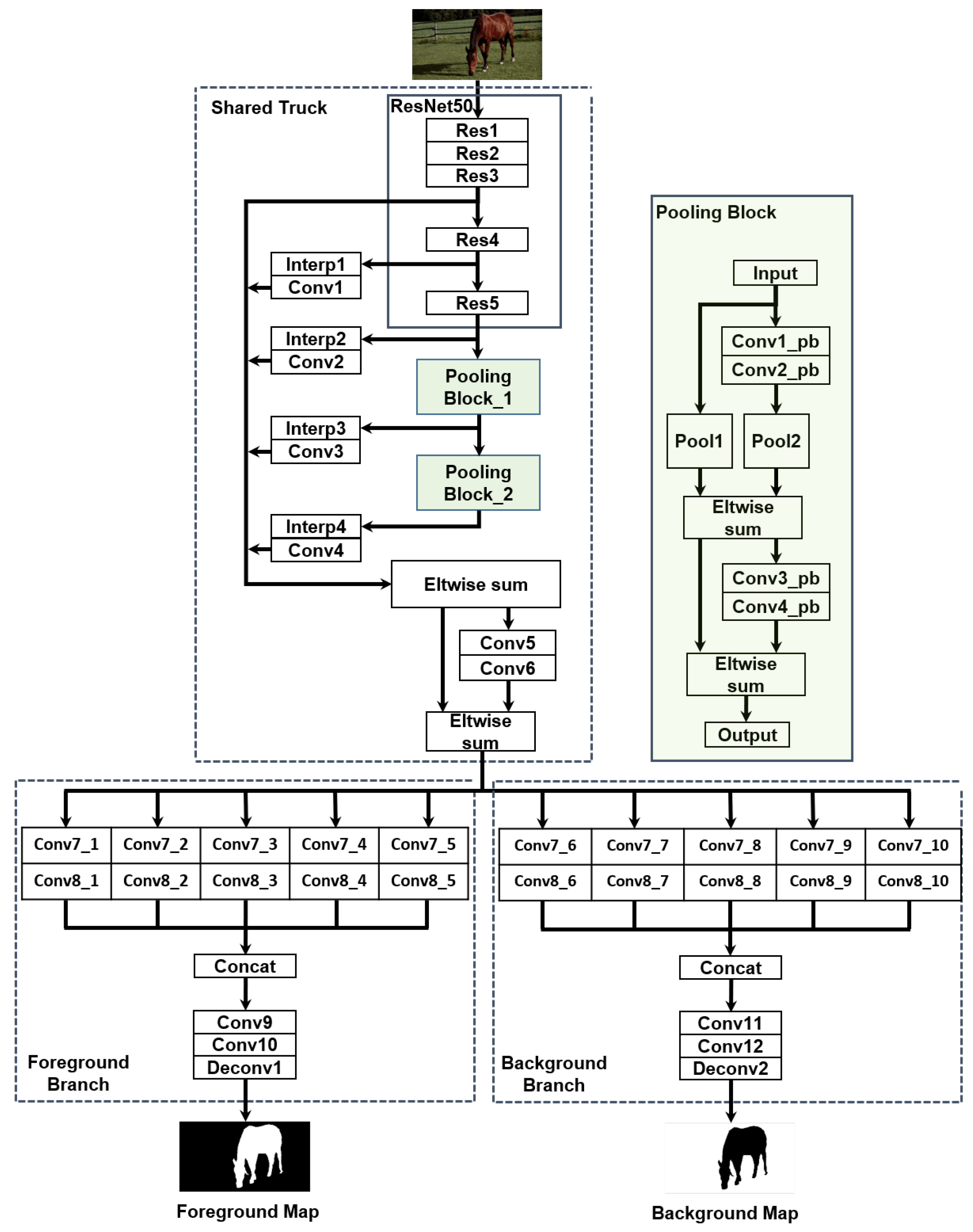
3.2. Deep Optimization with Complementary CNNs

Given the empirical loss (2) and the complementary loss (3), we can derive two models, ϕ F ( · ) and ϕ B ( · ) , for per-frame initialization of the foreground and background maps by solving the optimization problem of objective functions (1). Toward this end, we need to first determine the form of the models and the algorithm for optimizing their parameters. Considering the impressive capability of convolutional neural networks (CNN), we propose to solve the optimization problem in a deep learning paradigm.
The architecture of the proposed CNN can be found in Figure 3, which starts from a shared trunk and ends up with two separate branches, i.e., a foreground branch and a background branch. The main configurations and details are shown in Table 1. For simplicity, only the foreground branch is illustrated in Table 1, as the background one adopts the same architecture. Note that this network simultaneously handles two complementary tasks as well as their relationships and is denoted as a complementary segmentation network (CSNet). The parameters of the shared trunk are initialized from the ResNet50 networks [64], which are used to extract low- to high-level features that are shared by foreground objects and background distractors. We remove the pooling layer and the fully connected layer after the RELU layer of res5c and introduce two pooling blocks (see Figure 3) to provide features from additional levels and reduce parameters. In order to integrate both the local and global contexts, we sum up different levels of feature outputs by layer Res3, Res4 and Res5 and two pooling blocks by appropriate up/down-sampling operations. After that, a residual block with a 3 × 3 CONV layer and a 1 × 1 CONV layer is used to post-process the integrated features as well as increase their nonlinearity. Finally, the shared trunk takes a 320 × 320 image as the input and outputs a 40 × 40 feature map with 512 channels.
After the shared trunk, the features are fed into two separate branches that address two complementary tasks, i.e., foreground and background estimation. Note that the two branches share the architecture with the input, but produce complementary outputs. In each branch, the shared features pass through a sequential of convolution blocks. These blocks all consist of 1 × 1 and 3 × 3 CONVs, but with different dilations. As such, we concatenate the output of each block to constitute feature maps at 40 × 40 resolution with 1280 channels. These features, which have a wide range of spatial context and abstraction levels, are finally fed into several CONV layers for dimensional reduction and post-processing, and upsampled to produce output segmentation maps at size 161 × 161 . With such designs, the foreground branch mainly focuses on detecting salient objects, while the background one suppresses distractors. In addition to the empirical loss defined in (2), two additional losses, (4) and (5), are also adopted to penalize the conflicts and complementary degree of the output maps for more accurate predictions.
In the training stage, we collect massive images with labeled salient objects from four datasets for image-based salient object detection [5,46,65,66]. We down-sample all images to 320 × 320 and their ground-truth saliency maps into 161 × 161 . For the pretrained ResNet50 trunk, the learning rate is set to 5 × 10 7 , while for the two branches they are 5 × 10 6 . We train the network with a mini-batch of 4 images using the SGD optimizer with a momentum of 0.9 and a weight decay of 0.0005 .

4. Efficient Temporal Propagation with Neighborhood Reversible Flow

The per-frame initialization of foregroundness and backgroundness can only provide a location prediction of the primary objects and background distractors at the spatial domain. However, the concept of primary objects is defined from a more global spatiotemporal perspective, not only salient in the intra-frame but also consistent in the inter-frame and throughout the whole video. As mentioned earlier, the primary video object should be spatiotemporally consistent, i.e., the saliency foreground regions should not change dramatically along the time dimension. This implies that there still exists a large gap between the frame-based initialization results and the video-based primary objects. Therefore, we need to further infer the primary objects that consistently pop out in the whole video [15] according to the spatiotemporal correspondence of visual signals. In this process, two key challenges need to be addressed, including:
(1)
How to find the most reliable correspondences between various (nearby or far-away) frames;
(2)
How to infer out the consistent primary objects based on spatiotemporal correspondences and the initialization results?
To address these two challenges, we propose a neighborhood reversible flow algorithm to find and propagate a neighborhood reversible subset from the inter-frames. Details of our solutions will be discussed in the following part of this section.

4.1. Neighborhood Reversible Flow

The proposed neighborhood reversible flow (NRF) propagates information along reliable correspondences established among several key frames of the video, thus preventing errors from accumulating quickly and involving larger temporal windows for more effective context exploitation. Instead of pixel-level correspondence, NRF operates on superpixels to achieve region-level matching and higher computational efficiency.
Given a video V = { I u } u = 1 K , we first apply the SLIC algorithm [67] to divide a frame I u into N u superpixels, denoted as { O u i } . For each superpixel, we compute its average RGB, Lab and HSV colors as well as the horizontal and vertical positions. These features are then normalized into the same dynamic range [ 0 , 1 ] .
Based on the features, we need to address two fundamental problems: (1) how to measure the correspondence between a superpixel O u i from the frame I u and a superpixel O v j from the frame I v , and (2) which frames should be referred to for a given frame? Inspired by the concept of neighborhood reversibility in image search [68], we can compute the pair-wise 1 distances between { O u i } i = 1 N u and { O v j } j = 1 N v . After that, we denote the k-nearest neighbors of O u i in the frame I v as N k ( O u i | I v ) . As a consequence, two superpixels O u i and O v j are k-neighborhood reversible if they reside in the list of k-nearest neighbors of each other. That is,
O u i N k ( O v j | I u ) and O v j N k ( O u i | I v ) .
From (6), we find that the smaller the k, the more tightly two superpixels are temporally correlated. Therefore, the correspondence between O u i and O v j can be measured as
s u i , v j = exp ( 2 k / k 0 ) , if k k 0 0 , otherwise
where k 0 is a constant to suppress weak flow, and k is a variable. A small k 0 will build sparse correspondences between I u and I v (e.g., k 0 = 1 ), while a large k 0 will cause dense correspondences. In this study, we empirically set k 0 = 15 and represent the flow between I u and I v with a matrix F u v R N u × N v , in which the component at ( i , j ) equals f u i , v j . Note that we further normalize F u v so that each row sums up to 1. Considering the highly redundant visual content between adjacent frames, for each video frame I u , we pick up its adjacent keyframes { I t | t T u } to ensure sufficient variation in content and depict reliable temporal correspondences. In this paper, we refer to the interval d k of annotated video frames, which usually contain the most critical information of the whole video, to determine the interval of adjacent keyframes. Later, we estimate the flow matrixes between a frame I u and the frames { I t | t T u } , where T u can be empirically set to { u 2 × d k , u d k , u + d k , u + 2 × d k } .

4.2. Temporal Propagation of Spacial Features

The flow { F u v } depicts how superpixels in various frames are temporally correlated, which can be used to further propagate the spatial foregroundness and backgroundness. Typically, such temporal refinement can obtain impressive performance by solving a complex optimization problem with constraints like spatial compactness and temporal consistency. However, the time cost will also grow surprisingly high [20]. Considering the requirement of efficiency in many real-world applications, we propose to minimize an objective function that has an analytic solution. For a superpixel O u i , its foregroundness x u i and backgroundness y u i can be initialized as
x v j = p O u i X u ( p ) | O u i | , y u i = p O u i Y u ( p ) | O u i | ,
where p is a pixel with foregroundness X u ( p ) and backgroundness Y u ( p ) . | O u i | is the area of O u i . For the sake of simplification, we represent the foregroundness and backgroundness scores of all superpixels in the uth frame with column vectors x u and y u , respectively. As a result, we can propagate such scores from I v to I u according to F u v :
x u | v = F u v x v , y u | v = F u v y v , v T u .
After the propagation, the foregroundness vector x ^ u and backgroundness vector y ^ u can be refined by solving
x ^ u = arg min x x x u 2 2 + λ c v T u x x u | v 2 2 , y ^ u = arg min y y y u 2 2 + λ c v T u y y u | v 2 2 ,
where λ c is a positive constant whose value is empirically set to 0.5. Note that we adopt only the 2 norm in (10) so as to efficiently compute an analytic solution
x ^ u = 1 1 + λ c · | T u | x u + λ c v T u F u v x v , y ^ u = 1 1 + λ c · | T u | y u + λ c v T u F u v y v .
By observing (9) and (11), we find that the propagation process is actually calculating the average foregroundness and backgroundness scores within a local temporal slice under the guidance of neighborhood reversible flow. After the temporal propagation, we turn superpixel-based scores into pixel-based ones according to
M u ( p ) = i = 1 N u δ ( p O u i ) · x ^ u i · ( 1 y ^ u i ) ,
min x x x u 2 2 + λ c v T u x F u v x v 2 2
where M u is the importance map of I u that depict the presence of primary objects. δ ( p O u i ) is an indicator function, which equals 1 if p O u i and 0 otherwise. Finally, we calculate an adaptive threshold which equals the 20% of the maximal pixel importance to binarize each frame, and a morphological closing operation is then performed to fill in the black area in the segmented objects.

5. Experiments

In this section, we first illustrate experimental settings about datasets and evaluation metrics in Section 5.1. Then, based on the datasets and metrics, we quantitatively compare our primary video object segmentation method with 22 state-of-the-art approaches in Section 5.2. After that, in Section 5.3, we further demonstrate the effectiveness of our approach by offering more detailed exploration and dissecting various parts of our approach as well as running time and failure cases.

5.1. Experimental Settings

We test the proposed approach on three widely used video datasets; their ways of defining primary video objects are different. Details of these datasets are described as follows:
(1)
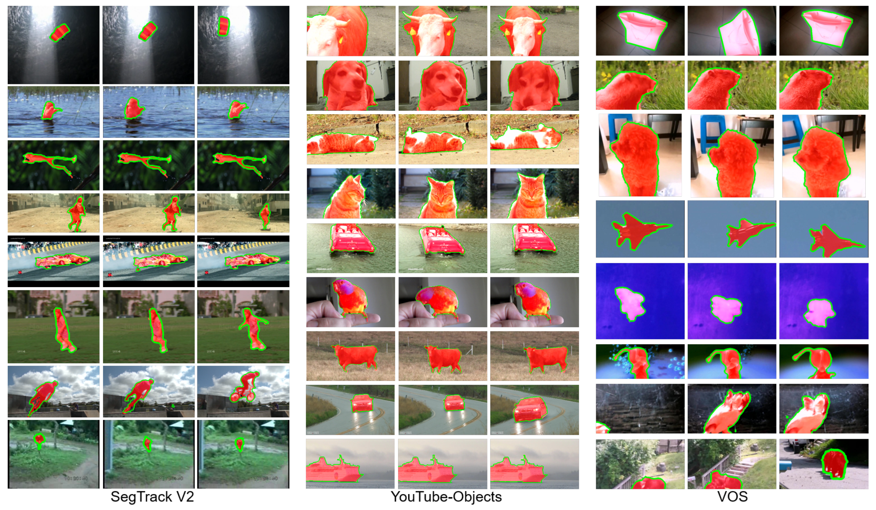
SegTrack V2 [59] is a classic dataset in video object segmentation that is frequently used in many previous works. It consists of 14 densely annotated video clips with 1066 frames in total. Most primary objects in this dataset are defined as ones with irregular motion patterns.
(2)
Youtube-Objects [1] contains a large amount of Internet videos, and we adopt its subset [69] that contains 127 videos with 20,977 frames. In these videos, 2153 keyframes are sparsely sampled and manually annotated with pixel-wise masks according to the video tags. In other words, primary objects in Youtube-Objects are defined from the perspective of semantic attributes.
(3)
VOS [15] contains 200 videos with 116,093 frames. On 7467 uniformly sampled keyframes, all objects are pre-segmented by 4 subjects, and the fixations of another 23 subjects are collected in eye-tracking tests. With these annotations, primary objects are automatically selected as the ones whose average fixation densities over the whole video fall above a predefined threshold. If no primary objects can be selected with the predefined threshold, objects that receive the highest average fixation density will be treated as the primary ones. Different from SegTrack V2 and Youtube-Objects, primary objects in VOS are defined from the perspective of human visual attention.
On these three datasets, the proposed approach, denoted as CSP, is compared with 22 state-of-the-art models for primary and salient object segmentation, including: RBD [34], SMD [70], MB+ [48], DRFI [2], BL [71], BSCA [47], MST [72], ELD [4], MDF [5], DCL [53], LEGS [13], MCDL [7] and RFCN [73], ACO [22], NLC [74], FST [23], SAG [57], GF [60], PN+ [75], DFI [76], FSal [77] and PFS [78].
In the comparisons, we adopt two sets of evaluation metrics, including the intersection-over-union (IoU) and the precision-recall- F β . Similar to [15], the precision, recall and IoU scores are first computed on each video and finally averaged over the whole dataset so as to generate the mean average precision (mAP), mean average recall (mAR) and mean average IoU (mIoU). In this manner, the influence of short and long videos can be balanced. Furthermore, a unique F β score can be obtained based on mAR, mAP and a parameter β , the square of which is set as 0.3 to emphasize precision more than recall in the evaluation.

5.2. Comparisons with State-of-the-Art Models

The performances of our approach and 22 state-of-the-art models on three video datasets are shown in Table 2. Some representative results of our approach are demonstrated in Figure 4. From Table 2, we find that on Youtube-Objects and VOS, for such larger datasets, our approach obtains the best F β and mIoU scores, while on SegTrack V2, our approach ranks the second place (worse than NLC). This can be explained by the fact that SegTrack V2 contains only 14 videos, among which most primary objects have irregular motion patterns. Such videos often perfectly meet the assumption of NLC on motion patterns of primary objects, making it the best approach on SegTrack V2. However, when the scenarios being processed extend to datasets such as VOS that are constructed without such “constraints” on motion patterns, the performance of NLC drops sharply, as its assumption may sometimes fail (e.g., VOS contains many videos only with static primary objects and distractors as well as slow camera motion; see Figure 4). These results further validate that it is quite necessary to conduct comparisons on larger datasets with daily videos (such as VOS) so that models with various kinds of assumptions can be fairly evaluated.
Moreover, there exist some approaches (BL and MB+) on the three datasets that outperform our approach in recall, and some other approaches (NLC, ACO, PN+ and FST) may achieve better or comparable precision with our approach on SegTrack V2. However, the other evaluation scores of the approaches are much worse than our method on the three datasets. That is, none of these approaches simultaneously outperforms our approach in both recall and precision, so our approach often has better overall performance, especially on larger datasets. This may imply that the proposed approach is more balanced than previous works. By analyzing the results on the three datasets, we find that this phenomenon may be caused by the conduction of complementary tasks in CSNet. By propagating both foregroundness and backgroundness, some missing foreground information may be retrieved, while the mistakenly popped-out distractors can be suppressed again, leading to balanced recall and precision.
From Table 2, we also find that there exist inherent correlations between salient image object detection and primary video object segmentation. As shown in Figure 4, primary objects are often the most salient ones in many frames, which explains why deep models such as ELD, RFCN and DCL outperform many video-based models such as NLC, SAG and GF. However, there are several key differences between the two problems. First, primary objects may not always be the most salient ones in all frames (as shown in Figure 1). Second, inter-frame correspondences provide additional cues for separating primary objects and distractors, which depict a new way to balance recall and precision. Third, primary objects may be sometimes close to the video boundary due to camera and object motion, making the boundary prior widely used in many salient object detection models not valid (e.g., the bear in the last row of the last column of Figure 4). Last but not least, salient object detection needs to distinguish a salient object from a fixed set of distractors, while primary object segmentation needs to consistently pop out the same primary object from a varying set of distractors. To sum up, primary video object segmentation is a more challenging task that needs to be further explored from the spatiotemporal perspective.

5.3. Detailed Performance Analysis

Beyond performance comparison, we also conduct several experiments on VOS, the largest one of the three datasets, to find out how the proposed approach works in segmenting primary video objects. Moreover, an additional metric, i.e., temporal stability measure T [14], is applied to evaluating the relevant aspect in primary video object segmentation in addition to the aforementioned four metrics. After all, mIoU only measures how well the pixels of two masks match, while F β measures the accuracy of contours. None of them consider the temporal aspect. However, video object segmentation is conducted in spatiotemporal dimensions. Therefore, the additional temporal stability measure is a appropriate choice to evaluate the temporal consistency of segmentation results. The main quantifiable results can be found in Table 3. In Table 3, the first group is our previous work in [39], and the second group is our current work extended from [39]. In order to illustrate the effect of each component in our approach, the two groups of tests are based on the same parameters, except for the last case, R-Init. + NRFp, which is the final test result obtained generally by using some data argumentations and parameter adjustments on the base of the case R-Init. + NRF.

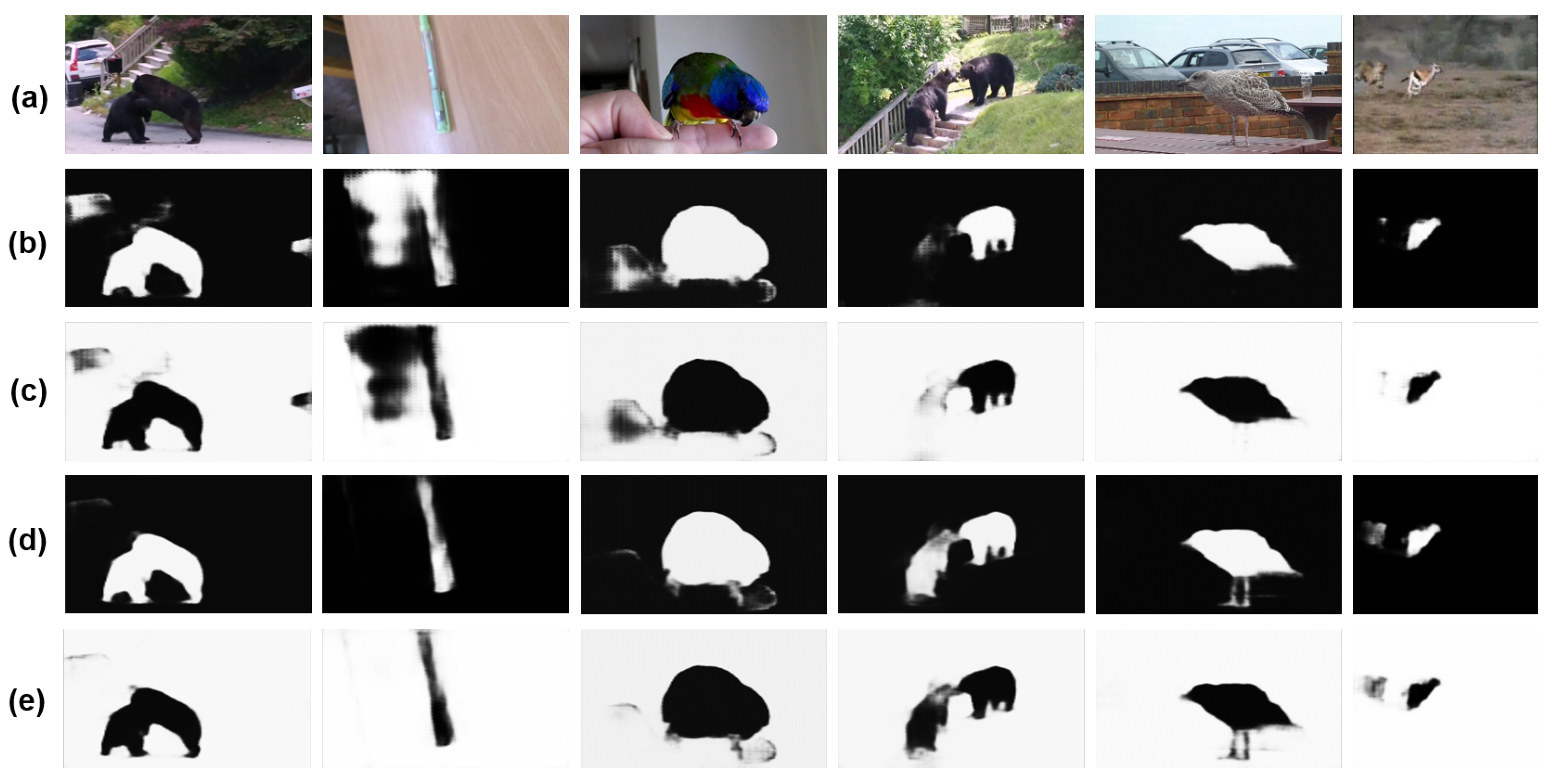
5.3.1. Performance of Complementary CNNs

In this section, some detail analysis will be given to further verify the effectiveness of the proposed complementary CNN branches and complementary loss.
Impact of two complementary branches. To explore the impact of two complementary network branches, we evaluated the foreground maps and background maps initialized by the two complementary branches, as well as their fusion maps. As shown in Table 3, in the first group the evaluation scores of case V-Init. FG and V-Init. BG are equally matched for their same branch structure, while the ones of their fusion maps increased to different degrees, which suggests that the complementary characteristics of initialized foreground maps and background maps can contribute to and constrain each other to generate more accurate prediction. Then what will happen if we abandon the background branch? To this end, we conducted two additional experiments in our previous work [39]. First, if we cut down the background branch and retrain only the foreground branch, the final performance decreases by about 0.9%. Second, if we re-train a network with two foreground branches, the final F β and mIoU scores decrease from 0.806 to 0.800 and 0.710 to 0.700, respectively. These experiments indicate that, beyond learning more weights, the background branch does learn some useful cues that are ignored by the foreground branch, which are expected to be high-level visual patterns of typical background distractors. These results also validate the idea of training deep networks by simultaneously handling two complementary tasks.
Therefore, network structures with two similar branches are still adopted in this extension work. What is different is that the new network structure is assisted with more designs based on the deeper and more effective ResNet50 instead of simple VGG16. From Table 3, we can find that the initialized results are distinctly improved when the backbone VGG16 is replaced by ResNet50. The aforementioned four evaluation scores are all increased, e.g., the F β and mIoU scores increase from 0.776 to 0.791 and 0.684 to 0.710, respectively, although the temporal stability performance is affected. This reveals the better performance of our new network structure, and at the same time, hints at the fact that a favourable per-frame initialization cannot stand for a good video initialization because of the temporal consistency attribute in video. Thus, it is necessary to conduct optimization in thhe temporal dimension, which will be explained in the next subsection.
Effect of the complementary loss. Except for the specific network, another main difference is that the two complementary CNN bracnches in CSNet are also constrained by our complementary loss. To verify the effectiveness, we optimize two sets of foreground and background prediction models based on the new network structure, one with the constraint of the penalty term in the objective function, and the other without. Based on the two sets of models, we can initialize a foreground and a background map for each video frame. The quantitative evaluations of initialization results respectively correspond to the cases R-Init. FGp/BGp/(FGp + BGp) and the cases R-Init. FG/BG/(FG + BG) in Table 3. From Table 3 we can find that, compared to the predictions without the penalty term constraint, the foreground and background models with the additional complementary loss can achieve better performance in predicting both foreground maps and background maps, shown as better F β and mIoU scores. Moreover, some visual examples are shown in Figure 5. Obviously, if we only use the empirical loss (2), some background regions may be wrongly classified into foreground (e.g., the first three columns in Figure 5), while some foreground details may be missed (e.g. the last three columns in Figure 5). By incorporating the additional complementary loss (3), these mistakes can be fixed (see Figure 5d,e). Thus, the complementary loss is effective for boundary localization and suppressing background distractors. These results validate the effectiveness of handling two complementary tasks with explicit consideration of their relationships.
Combining the two differences, the F β and mIoU scores of initialization results output by our previous network CCNN (the case V-Init. (FG + BK)) increase by about 3.6% and 7.2%, i.e., from 0.800 to 0.829 and 0.689 to 0.739, respectively, with the increased mAP and mAR scores. This also means that the combination of complementary loss and two complementary branches of foreground and background are valid and ingenious.
In particular, the complementary CNN branches in our two networks both show impressive performance in predicting primary video objects over the other 6 deep models when their pixel-wise predictions are directly evaluated on VOS. By analyzing the results, we find that this may be caused by two reasons: (1) using more training data, and (2) simultaneously handling complementary tasks, whose effectiveness is just verified. To explore the first reason, we retrained the CCNN on the same MSRA10K dataset used by most deep models. In this case, the F β (mIoU) scores of the foreground and background maps predicted by CCNN decrease to 0.747 (0.659) and 0.745 (0.658), respectively. Note that both branches still outperform RFCN on VOS in terms of mIoU (but F β is slightly worse).

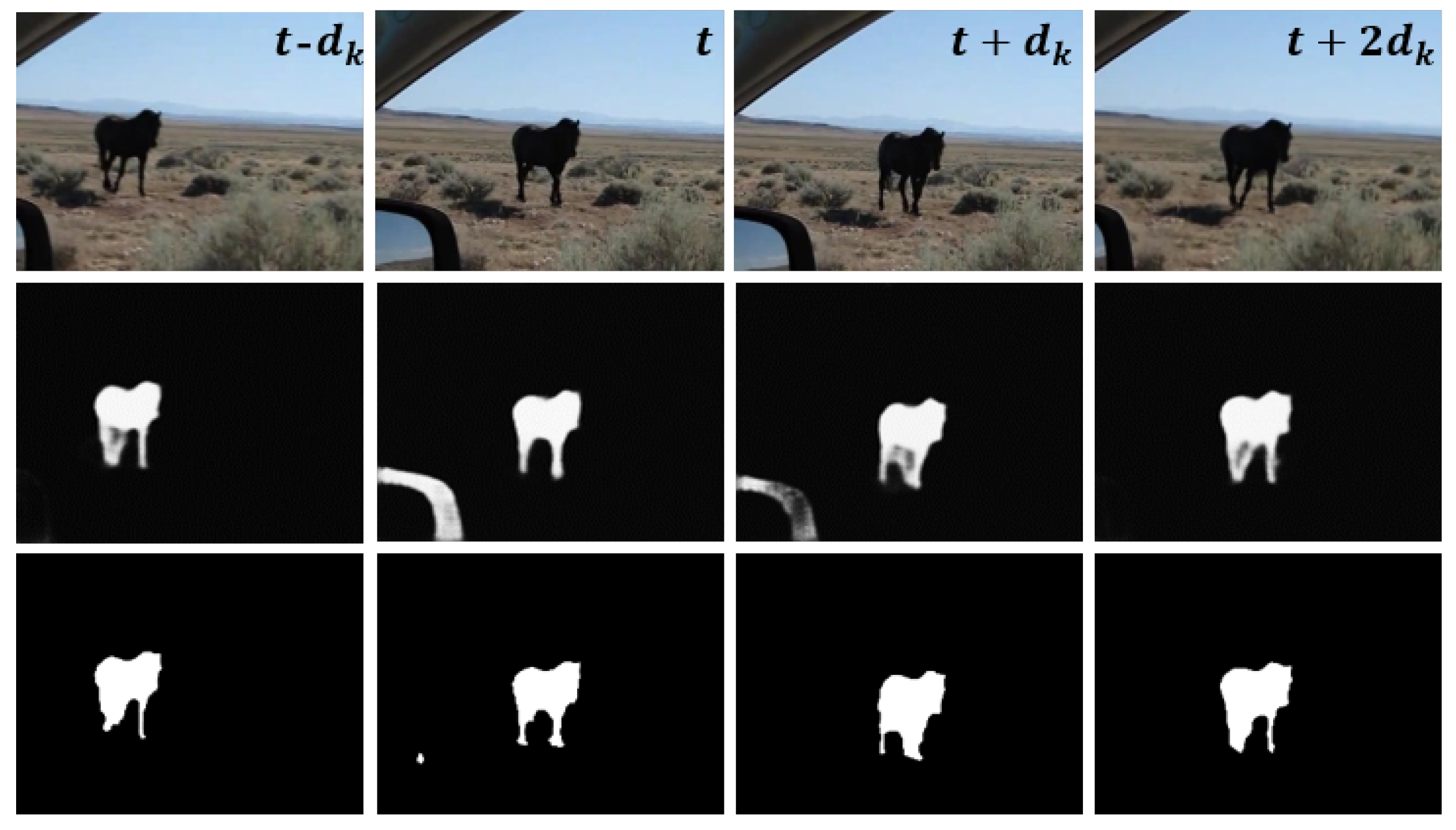
5.3.2. Effectiveness of Neighborhood Reversible Flow

Through the above complementary network branches, the salient foreground and background maps in the intra-frame are well obtained, while the initialization operation cannot ensure the temporal consistency of segmented objects, e.g., the initialized predictions by CSNet outperform the ones by the CCNN in term of mAP, mAR, F β and mIoU but become inferior in temporal stability mT. Thus, the thought of improving the temporal relationship was proposed in Section 4, i.e., finding and propagating the reliable inter-frame correspondences by applying the neighborhood reversible flow to make the consistent salient subsets enhanced and accidental distractors suppressed. Consequently, the final primary video objects with spatiotemporal consistency are yielded.
Effectiveness of Neighborhood Reversible Flow. To prove this thought, we compare the initialized results by CCNN (CSNet) with the optimized results (V-Init.(R-Init.) + NRF) by neighborhood reversible flow. As shown in Table 3, the temporal stability measure mT of optimization results in CCNN (CSNet) cases decrease from 0.121 (0.122) to 0.109 (0.108) compared with the initialized predictions (V-Init. (FG + BK), R-Init. (FGp + BKp)). At the same time, the other evaluation scores are also improved, e.g., the mIoU score increases from 0.689 to 0.710. The superiority will become more obvious if we directly compare V-Init. + NRF with V-Init. FG, i.e., conduct the fusion operation on foreground and background in the process of neighborhood reversible flow just like we really do. This means that by propagating the neighborhood reversible flow, the spatial subsets of primary objects in intra-frame can be refined from a temporal perspective, and the inter-frame temporal consistency can be enhanced. Finally, the primary video objects with favourable spatiotemporal consistency can pop out. As shown in Figure 6, the primary objects in most video frames are initialized as the horce, while the objects that only lasts for a short while are mistakenly classified into foreground due to their spatial saliency in certain frames. Fortunately, the distractors are well suppressed by the optimization of neighborhood reversible flow (see the third rows in Figure 6). Thus, via propagating salient cues in inter-frames, background objects could be effectively suppressed, only preserving the real primary one.
To further demonstrate the effectiveness of neighborhood reversible flow, we tested our approach with two new settings based on the CCNN. In the first setting, we replaced the correspondence from Equation (7) with the cosine similarity between superpixels. In this case, the F β and mIoU scores of our approach on VOS drop to 0.795 and 0.696, respectively. Such performance is still better than the initialized foreground maps but worse than the performance when using the neighborhood reversible flow ( F β = 0.806, mIoU = 0.710). This result indicates the effectiveness of neighborhood reversibility in temporal propagation.
In the second setting, we set λ c = + in Equation (10), implying that primary objects in a frame are solely determined by the foreground and background propagated from other frames. When the spatial predictions of each frame are actually ignored in the optimization process, the F β (mIoU) scores of our approach on VOS only decrease from 0.806 (0.710) to 0.790 (0.693), respectively. This result proves that the inter-frame correspondences encoded in the neighborhood reversible flow are quite reliable for efficient and accurate propagation along the temporal dimension.
It is worth mentioning that in the previous initialization process, the predictions are all pixel-wise, while the temporal optimization via neighborhood reversible flow is conducted on superpixel wise foreground/background maps in order to reduce time consumption, i.e., the predictions need to be converted from the pixel to superpixel and finally converted to pixel. However, the superpixel-wise predictions are relatively coarse and may affect the following process. To explore this effect, we converted the foreground/background maps and their fusion maps in cases R-Init. FGp/BKp from pixel-wise to superpixel-wise, as shown in Table 4. Fortunately, both F β and mIoU scores of foreground (background) maps only slightly decrease by 0.003 (0.004), and the mT scores increase by 0.009, while the negative effect on fusion maps mainly manifests in mT scores, which can be improved by the propagation of neighborhood reversible flow. Thus, the trade-off is worthy. This also hints at the important effect of neighborhood reversible flow on temporal stability or consistency.
Parameter setting. In the experiment based on CCNN, we smoothly varied two key parameters used in NRF, including the k 0 in constructing neighborhood flow and the λ c that controls the strength of temporal propagation. As shown in Figure 7, a larger k 0 tends to bring slightly better performance, while our approach performs the best when λ c = 0.5 . In these experiments, we set k 0 = 15 and λ c = 0.5 when constructing the neighborhood reversible flow.
Selection of color spaces. In constructing the flow, we represented each superpixel with three color spaces. As shown in Table 5, a single color space performs slightly worse than their combinations. Actually, using multiple color spaces has been proved to be useful in detecting salient objects [2], as multiple color spaces make it possible to assess temporal correspondences from several perspectives with a small increase in time cost. Therefore, we choose to use RGB, Lab and HSV color spaces in characterizing a superpixel.

5.3.3. Running Time

We tested the speed of the proposed approach with a 3.4 GHz CPU (only using single thread) and an NVIDIA TITAN Xp GPU (without batch processing). The average time costs of each key step of our approach in processing 400 × 224 frames are shown in Table 6. Note that the majority of the implementation runs on the Matlab platform, with several key steps written in C (e.g., superpixel segmentation and feature conversion between pixels and superpixels). We find that our approach takes only 0.20 s to process a frame if not using multi-test, and no more than 0.75 s even using multi-test, which is much faster than many video-based models (e.g., 19.0 s for NLC, 6.1 s for ACO, 5.8 s for FST, 5.4 s for SAG and 4.7 s for GF). This may be caused by the fact that we only build correspondences on superpixels with the neighborhood reversibility, which is very efficient. Moreover, we avoid using complex optimization objectives and constraints. Instead, we use only simple quadratic optimization objectives so as to obtain analytic solutions. The high efficiency of our approach makes it possible to be used in some real-world applications.

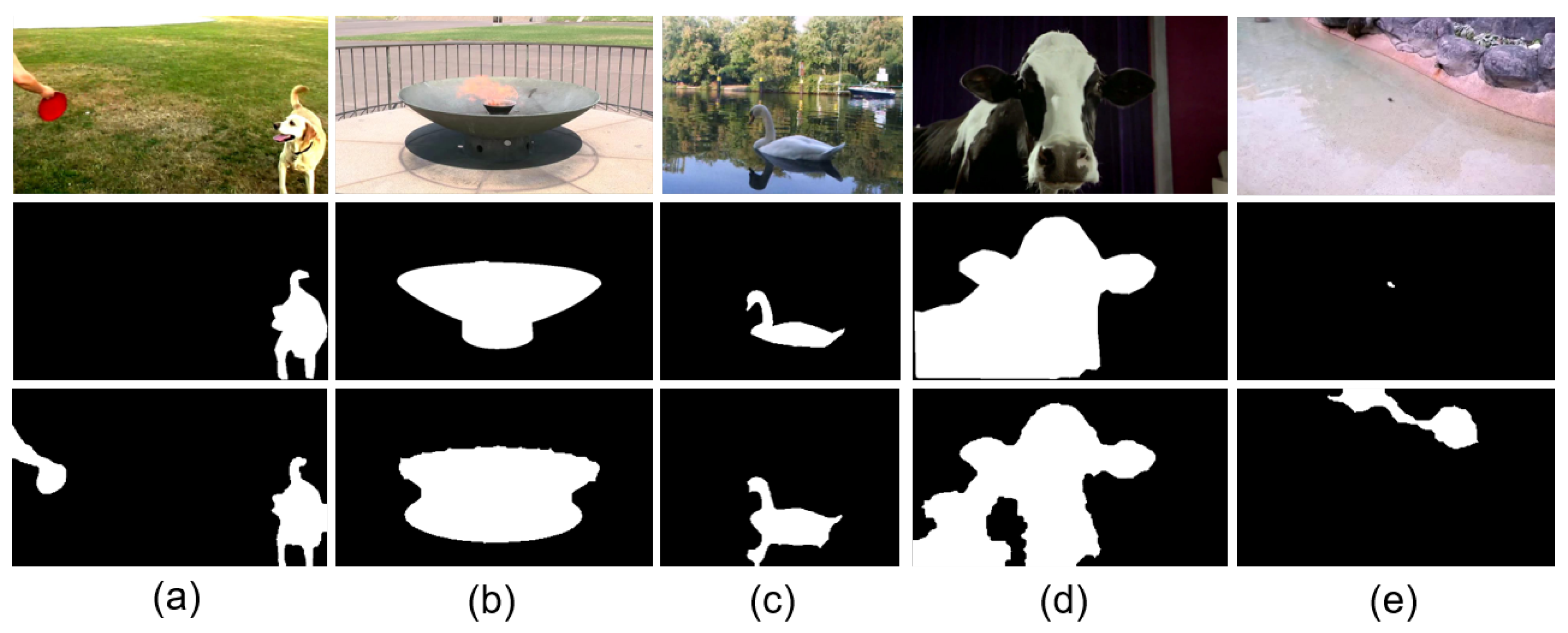
5.3.4. Failure Cases

Beyond the successful cases, we also show in Figure 8 some failures. We find that failures can be caused by the way of defining primary objects. For example, the salient hand in Figure 8a is not labeled as a primary object, as the corresponding videos from Youtube-Objects are tagged with “dog”. Moreover, shadows (Figure 8b) and reflections (Figure 8c) generated by the target object and environment are some other reasons that may cause unexpected failures due to their similar saliency with the target object. It is also easy to fail when parts of the regions of the target salient object are similar to the background (Figure 8d). Specifically, successful segmentation is very hard for some minuscule objects, e.g., a crab in water (Figure 8e). Such failures need further exploration in the future.

6. Conclusions

In this paper, we propose a simple yet effective approach for primary video object segmentation. Based on the complementary relationship of the foreground and the background, the problem of primary object segmentation is turned into an optimization problem of objective function. According to the proposed objective function, a complementary convolutional neural network is designed and trained on massive images from salient object datasets to handle complementary tasks. Then, by the trained models, the foreground and background in a video frame can be effectively predicted from the spatial perspective. After that, such spatial predictions are efficiently propagated via the inter-frame flow that has the characteristic of neighborhood reversibility. In this manner, primary objects in different frames can gradually pop out, while various types of distractors can be well suppressed. Extensive experiments on three video datasets have validated the effectiveness of the proposed approach.
In the future work, we intend to improve the proposed approach by fusing multiple methods of defining primary video objects such as motion patterns, semantic tags and human visual attention. Moreover, we will try to develop a completely end-to-end spatiotemporal model for primary video object segmentation by incorporating the recursive mechanism.

Author Contributions

Methodology, J.W. and J.L.; Project administration, J.W.; Validation, L.X.; Writing—original draft, J.W.; Writing—review & editing, J.L. and L.X. All authors have read and agreed to the published version of the manuscript.

Funding

This research was funded by the National Natural Science Foundation of China under grant number 62132002 and 11790305.

Institutional Review Board Statement

Not applicable.

Informed Consent Statement

Not applicable.

Data Availability Statement

Not applicable.

Conflicts of Interest

The authors declare no conflict of interest.

References

  1. Prest, A.; Leistner, C.; Civera, J.; Schmid, C.; Ferrari, V. Learning object class detectors from weakly annotated video. In Proceedings of the 2012 IEEE Conference on Computer Vision and Pattern Recognition, Providence, RI, USA, 16–21 June 2012; pp. 3282–3289. [Google Scholar]
  2. Jiang, H.; Wang, J.; Yuan, Z.; Wu, Y.; Zheng, N.; Li, S. Salient object detection: A discriminative regional feature integration approach. In Proceedings of the IEEE Conference on Computer Vision and Pattern Recognition (CVPR), Portland, OR, USA, 23–28 June 2013; pp. 2083–2090. [Google Scholar]
  3. Zhang, D.; Meng, D.; Han, J. Co-saliency detection via a self-paced multiple-instance learning framework. IEEE Trans. Pattern Anal. Mach. Intell. 2016, 39, 865–878. [Google Scholar] [CrossRef] [PubMed]
  4. Lee, G.; Tai, Y.W.; Kim, J. Deep saliency with encoded low level distance map and high level features. In Proceedings of the IEEE Conference on Computer Vision and Pattern Recognition, Las Vegas, NV, USA, 27–30 June 2016; pp. 660–668. [Google Scholar]
  5. Li, G.; Yu, Y. Visual saliency based on multiscale deep features. In Proceedings of the IEEE Conference on Computer Vision and Pattern Recognition, Boston, MA, USA, 7–12 June 2015; pp. 5455–5463. [Google Scholar]
  6. Fan, D.P.; Li, T.; Lin, Z.; Ji, G.P.; Zhang, D.; Cheng, M.M.; Fu, H.; Shen, J. Re-thinking co-salient object detection. IEEE Trans. Pattern Anal. Mach. Intell. 2021, 44, 4339–4354. [Google Scholar] [CrossRef] [PubMed]
  7. Zhao, R.; Ouyang, W.; Li, H.; Wang, X. Saliency detection by multi-context deep learning. In Proceedings of the IEEE Conference on Computer Vision and Pattern Recognition, Boston, MA, USA, 7–12 June 2015; pp. 1265–1274. [Google Scholar]
  8. Zhuge, M.; Fan, D.P.; Liu, N.; Zhang, D.; Xu, D.; Shao, L. Salient object detection via integrity learning. IEEE Trans. Pattern Anal. Mach. Intell. 2022. [Google Scholar] [CrossRef] [PubMed]
  9. Wang, G.; Chen, C.; Fan, D.; Hao, A.; Qin, H. Weakly Supervised Visual-Auditory Saliency Detection with Multigranularity Perception. arXiv 2021, arXiv:2112.13697. [Google Scholar]
  10. Fan, D.P.; Zhang, J.; Xu, G.; Cheng, M.M.; Shao, L. Salient objects in clutter. IEEE Trans. Pattern Anal. Mach. Intell. 2022. [Google Scholar] [CrossRef]
  11. Zhao, J.X.; Liu, J.J.; Fan, D.P.; Cao, Y.; Yang, J.; Cheng, M.M. EGNet: Edge guidance network for salient object detection. In Proceedings of the IEEE/CVF International Conference on Computer Vision, Seoul, Korea, 27–28 October 2019; pp. 8779–8788. [Google Scholar]
  12. Fan, D.P.; Cheng, M.M.; Liu, J.J.; Gao, S.H.; Hou, Q.; Borji, A. Salient objects in clutter: Bringing salient object detection to the foreground. In Proceedings of the European Conference on Computer Vision (ECCV), Munich, Germany, 8–14 September 2018; pp. 186–202. [Google Scholar]
  13. Wang, L.; Lu, H.; Ruan, X.; Yang, M.H. Deep networks for saliency detection via local estimation and global search. In Proceedings of the IEEE Conference on Computer Vision and Pattern Recognition, Boston, MA, USA, 7–12 June 2015; pp. 3183–3192. [Google Scholar]
  14. Perazzi, F.; Pont-Tuset, J.; McWilliams, B.; Van Gool, L.; Gross, M.; Sorkine-Hornung, A. A Benchmark Dataset and Evaluation Methodology for Video Object Segmentation. In Proceedings of the IEEE Conference on Computer Vision and Pattern Recognition, Las Vegas, NV, USA, 27–30 June 2016. [Google Scholar]
  15. Li, J.; Xia, C.; Chen, X. A benchmark dataset and saliency-guided stacked autoencoders for video-based salient object detection. IEEE Trans. Image Process. 2018, 27, 349–364. [Google Scholar] [CrossRef] [Green Version]
  16. Maerki, N.; Perazzi, F.; Wang, O.; Sorkine-Hornung, A. Bilateral space video segmentation. In Proceedings of the IEEE Conference on Computer Vision and Pattern Recognition, Las Vegas, NV, USA, 27–30 June 2016. [Google Scholar]
  17. Ramakanth, S.A.; Babu, R.V. SeamSeg: Video object segmentation using patch seams. In Proceedings of the IEEE Conference on Computer Vision and Pattern Recognition, Columbus, OH, USA, 23–28 June 2014; pp. 376–383. [Google Scholar] [CrossRef]
  18. Seguin, G.; Bojanowski, P.; Lajugie, R.; Laptev, I. Instance-level video segmentation from object tracks. In Proceedings of the IEEE Conference on Computer Vision and Pattern Recognition, Las Vegas, NV, USA, 27–30 June 2016. [Google Scholar]
  19. Tsai, Y.H.; Zhong, G.; Yang, M.H. Semantic co-segmentation in videos. In Proceedings of the 14th European Conference on Computer Vision, Munich, Germany, 8–14 September 2016. [Google Scholar]
  20. Zhang, Y.; Chen, X.; Li, J.; Wang, C.; Xia, C. Semantic object segmentation via detection in weakly labeled video. In Proceedings of the IEEE Conference on Computer Vision and Pattern Recognition, Boston, MA, USA, 7–12 June 2015; pp. 3641–3649. [Google Scholar]
  21. Zhang, D.; Javed, O.; Shah, M. Video Object Segmentation through Spatially Accurate and Temporally Dense Extraction of Primary Object Regions. In Proceedings of the IEEE Conference on Computer Vision and Pattern Recognition, Portland, OR, USA, 23–28 June 2013; pp. 628–635. [Google Scholar] [CrossRef] [Green Version]
  22. Jang, W.D.; Lee, C.; Kim, C.S. Primary object segmentation in videos via alternate convex optimization of foreground and background distributions. In Proceedings of the IEEE Conference on Computer Vision and Pattern Recognition, Las Vegas, NV, USA, 27–30 June 2016; pp. 696–704. [Google Scholar]
  23. Papazoglou, A.; Ferrari, V. Fast object segmentation in unconstrained video. In Proceedings of the IEEE International Conference on Computer Vision, Portland, OR, USA, 23–28 June 2013; pp. 1777–1784. [Google Scholar]
  24. Xiao, F.; Jae Lee, Y. Track and segment: An iterative unsupervised approach for video object proposals. In Proceedings of the IEEE Conference on Computer Vision and Pattern Recognition, Las Vegas, NV, USA, 27–30 June 2016; pp. 933–942. [Google Scholar]
  25. Ji, G.P.; Fu, K.; Wu, Z.; Fan, D.P.; Shen, J.; Shao, L. Full-duplex strategy for video object segmentation. In Proceedings of the IEEE/CVF International Conference on Computer Vision, Montreal, BC, Canada, 10–17 October 2021; pp. 4922–4933. [Google Scholar]
  26. Fan, D.P.; Wang, W.; Cheng, M.M.; Shen, J. Shifting More Attention to Video Salient Object Detection. In Proceedings of the IEEE/CVF Conference on Computer Vision and Pattern Recognition (CVPR), Long Beach, CA, USA, 15–20 June 2019. [Google Scholar]
  27. Chiu, W.C.; Fritz, M. Multi-class video co-segmentation with a generative multi-video model. In Proceedings of the IEEE Conference on Computer Vision and Pattern Recognition, Portland, OR, USA, 23–28 June 2013; pp. 321–328. [Google Scholar] [CrossRef] [Green Version]
  28. Fu, H.; Xu, D.; Zhang, B.; Lin, S.; Ward, R.K. Object-based multiple foreground video co-segmentation via multi-state selection graph. IEEE Trans. Image Process. 2015, 24, 3415–3424. [Google Scholar] [CrossRef]
  29. Zhang, D.; Javed, O.; Shah, M. Video object co-segmentation by regulated maximum weight cliques. In Proceedings of the 13th European Conference on Computer Vision, Zurich, Switzerland, 6–12 September 2014; pp. 551–566. [Google Scholar]
  30. Yu, C.P.; Le, H.; Zelinsky, G.; Samaras, D. Efficient video segmentation using parametric graph partitioning. In Proceedings of the IEEE International Conference on Computer Vision, Santiago, Chile, 7–13 December 2015; pp. 3155–3163. [Google Scholar]
  31. Wang, W.; Shen, J.; Yang, R.; Porikli, F. Saliency-aware video object segmentation. IEEE Trans. Pattern Anal. Mach. Intell. 2018, 40, 20–33. [Google Scholar] [CrossRef]
  32. Cheng, M.M.; Mitra, N.J.; Huang, X.; Torr, P.H.; Hu, S.M. Global contrast based salient region detection. IEEE Trans. Pattern Anal. Mach. Intell. 2015, 37, 569–582. [Google Scholar] [CrossRef] [Green Version]
  33. Jiang, P.; Ling, H.; Yu, J.; Peng, J. Salient region detection by ufo: Uniqueness, focusness and objectness. In Proceedings of the IEEE International Conference on Computer Vision, Portland, OR, USA, 23–28 June 2013; pp. 1976–1983. [Google Scholar]
  34. Zhu, W.; Liang, S.; Wei, Y.; Sun, J. Saliency Optimization from Robust Background Detection. In Proceedings of the IEEE Conference on Computer Vision and Pattern Recognition, Columbus, OH, USA, 23–28 June 2014. [Google Scholar]
  35. Zhang, J.; Sclaroff, S. Saliency detection: A boolean map approach. In Proceedings of the IEEE International Conference on Computer Vision, Portland, OR, USA, 23–28 June 2013; pp. 153–160. [Google Scholar]
  36. Ge, W.; Guo, Z.; Dong, Y.; Chen, Y. Dynamic background estimation and complementary learning for pixel-wise foreground/background segmentation. Pattern Recognit. 2016, 59, 112–125. [Google Scholar] [CrossRef]
  37. Koh, Y.J.; Kim, C.S. Primary Object Segmentation in Videos Based on Region Augmentation and Reduction. In Proceedings of the 2017 IEEE Conference on Computer Vision and Pattern Recognition (CVPR), Honolulu, HI, USA, 21–26 July 2017; Volume 1, p. 7. [Google Scholar]
  38. Tsai, Y.H.; Yang, M.H.; Black, M.J. Video segmentation via object flow. In Proceedings of the IEEE Conference on Computer Vision and Pattern Recognition, Las Vegas, NV, USA, 27–30 June 2016; pp. 3899–3908. [Google Scholar]
  39. Li, J.; Zheng, A.; Chen, X.; Zhou, B. Primary video object segmentation via complementary cnns and neighborhood reversible flow. In Proceedings of the IEEE International Conference on Computer Vision, Venice, Italy, 22–29 October 2017; pp. 1417–1425. [Google Scholar]
  40. Liu, H.; Jiang, S.; Huang, Q.; Xu, C.; Gao, W. Region-based visual attention analysis with its application in image browsing on small displays. In Proceedings of the 15th ACM International Conference on Multimedia, Augsburg, Germany, 24–29 September 2007; pp. 305–308. [Google Scholar]
  41. Perazzi, F.; Krähenbühl, P.; Pritch, Y.; Hornung, A. Saliency filters: Contrast based filtering for salient region detection. In Proceedings of the 2012 IEEE Conference on Computer Vision and Pattern Recognition, Providence, RI, USA, 16–21 June 2012; pp. 733–740. [Google Scholar]
  42. Goferman, S.; Zelnik-Manor, L.; Tal, A. Context-aware saliency detection. IEEE Trans. Pattern Anal. Mach. Intell. 2012, 34, 1915–1926. [Google Scholar] [CrossRef] [Green Version]
  43. Wei, Y.; Wen, F.; Zhu, W.; Sun, J. Geodesic saliency using background priors. In Proceedings of the 12th European Conference on Computer Vision, Florence, Italy, 7–13 October 2012; pp. 29–42. [Google Scholar]
  44. Schauerte, B.; Stiefelhagen, R. Quaternion-based spectral saliency detection for eye fixation prediction. In Proceedings of the 12th European Conference on Computer Vision, Florence, Italy, 7–13 October 2012; pp. 116–129. [Google Scholar]
  45. Liu, T.; Yuan, Z.; Sun, J.; Wang, J.; Zheng, N.; Tang, X.; Shum, H.Y. Learning to detect a salient object. IEEE Trans. Pattern Anal. Mach. Intell. 2011, 33, 353–367. [Google Scholar]
  46. Yang, C.; Zhang, L.; Lu, H.; Ruan, X.; Yang, M.H. Saliency detection via graph-based manifold ranking. In Proceedings of the IEEE Conference on Computer Vision and Pattern Recognition, Portland, OR, USA, 23–28 June 2013; pp. 3166–3173. [Google Scholar]
  47. Qin, Y.; Lu, H.; Xu, Y.; Wang, H. Saliency detection via cellular automata. In Proceedings of the IEEE Conference on Computer Vision and Pattern Recognition, Boston, MA, USA, 7–12 June 2015; pp. 110–119. [Google Scholar]
  48. Zhang, J.; Sclaroff, S.; Lin, Z.; Shen, X.; Price, B.; Mech, R. Minimum barrier salient object detection at 80 fps. In Proceedings of the IEEE International Conference on Computer Vision, Santiago, Chile, 7–13 December 2015; pp. 1404–1412. [Google Scholar]
  49. Li, X.; Zhao, L.; Wei, L.; Yang, M.H.; Wu, F.; Zhuang, Y.; Ling, H.; Wang, J. Deepsaliency: Multi-task deep neural network model for salient object detection. IEEE Trans. Image Process. 2016, 25, 3919–3930. [Google Scholar] [CrossRef] [Green Version]
  50. Long, J.; Shelhamer, E.; Darrell, T. Fully convolutional networks for semantic segmentation. In Proceedings of the IEEE Conference on Computer Vision and Pattern Recognition, Boston, MA, USA, 7–12 June 2015; pp. 3431–3440. [Google Scholar]
  51. Liu, N.; Han, J. Dhsnet: Deep hierarchical saliency network for salient object detection. In Proceedings of the IEEE Conference on Computer Vision and Pattern Recognition, Las Vegas, NV, USA, 27–30 June 2016; pp. 678–686. [Google Scholar]
  52. Kuen, J.; Wang, Z.; Wang, G. Recurrent attentional networks for saliency detection. In Proceedings of the IEEE Conference on Computer Vision and Pattern Recognition, Las Vegas, NV, USA, 27–30 June 2016; pp. 3668–3677. [Google Scholar]
  53. Li, G.; Yu, Y. Deep contrast learning for salient object detection. In Proceedings of the IEEE Conference on Computer Vision and Pattern Recognition, Las Vegas, NV, USA, 27–30 June 2016; pp. 478–487. [Google Scholar]
  54. Yu, H.; Li, J.; Tian, Y.; Huang, T. Automatic interesting object extraction from images using complementary saliency maps. In Proceedings of the 18th ACM International Conference on Multimedia, Firenze, Italy, 25–29 October 2010; pp. 891–894. [Google Scholar]
  55. Tian, Y.; Li, J.; Yu, S.; Huang, T. Learning complementary saliency priors for foreground object segmentation in complex scenes. Int. J. Comput. Vis. 2015, 111, 153–170. [Google Scholar] [CrossRef]
  56. Liu, Z.; Zhang, X.; Luo, S.; Le Meur, O. Superpixel-based spatiotemporal saliency detection. IEEE Trans. Circuits Syst. Video Technol. 2014, 24, 1522–1540. [Google Scholar] [CrossRef]
  57. Wang, W.; Shen, J.; Porikli, F. Saliency-aware geodesic video object segmentation. In Proceedings of the IEEE Conference on Computer Vision and Pattern Recognition, Boston, MA, USA, 7–12 June 2015; pp. 3395–3402. [Google Scholar]
  58. Ochs, P.; Malik, J.; Brox, T. Segmentation of moving objects by long term video analysis. IEEE Trans. Pattern Anal. Mach. Intell. 2014, 36, 1187–1200. [Google Scholar] [CrossRef] [Green Version]
  59. Li, F.; Kim, T.; Humayun, A.; Tsai, D.; Rehg, J.M. Video segmentation by tracking many figure-ground segments. In Proceedings of the IEEE International Conference on Computer Vision, Portland, OR, USA, 23–28 June 2013; pp. 2192–2199. [Google Scholar]
  60. Wang, W.; Shen, J.; Shao, L. Consistent video saliency using local gradient flow optimization and global refinement. IEEE Trans. Image Process. 2015, 24, 4185–4196. [Google Scholar] [CrossRef] [Green Version]
  61. Nilsson, D.; Sminchisescu, C. Semantic video segmentation by gated recurrent flow propagation. arXiv 2016, arXiv:1612.08871. [Google Scholar]
  62. Gadde, R.; Jampani, V.; Gehler, P.V. Semantic video cnns through representation warping. CoRR 2017, 8, 9. [Google Scholar]
  63. Zhu, X.; Xiong, Y.; Dai, J.; Yuan, L.; Wei, Y. Deep feature flow for video recognition. In Proceedings of the IEEE Conference on Computer Vision and Pattern Recognition, Honolulu, HI, USA, 21–26 July 2017; Volume 1, p. 3. [Google Scholar]
  64. He, K.; Zhang, X.; Ren, S.; Sun, J. Deep residual learning for image recognition. In Proceedings of the IEEE Conference on Computer Vision and Pattern Recognition, Las Vegas, NV, USA, 27–30 June 2016; pp. 770–778. [Google Scholar]
  65. MSRA10K. Available online: http://mmcheng.net/gsal/ (accessed on 1 January 2016).
  66. Yan, Q.; Xu, L.; Shi, J.; Jia, J. Hierarchical Saliency Detection. In Proceedings of the IEEE Conference on Computer Vision and Pattern Recognition, Portland, OR, USA, 23–28 June 2013; pp. 1155–1162. [Google Scholar] [CrossRef] [Green Version]
  67. Achanta, R.; Shaji, A.; Smith, K.; Lucchi, A.; Fua, P.; Süsstrunk, S. SLIC Superpixels Compared to State-of-the-art Superpixel Methods. IEEE Trans. Pattern Anal. Mach. Intell. 2012, 34, 2274–2282. [Google Scholar] [CrossRef] [Green Version]
  68. Jegou, H.; Schmid, C.; Harzallah, H.; Verbeek, J. Accurate image search using the contextual dissimilarity measure. IEEE Trans. Pattern Anal. Mach. Intell. 2010, 32, 2–11. [Google Scholar] [CrossRef] [Green Version]
  69. Jain, S.D.; Grauman, K. Supervoxel-consistent foreground propagation in video. In Proceedings of the 13th European Conference on Computer Vision, Zurich, Switzerland, 6–12 September 2014; pp. 656–671. [Google Scholar]
  70. Peng, H.; Li, B.; Ling, H.; Hu, W.; Xiong, W.; Maybank, S.J. Salient object detection via structured matrix decomposition. IEEE Trans. Pattern Anal. Mach. Intell. 2017, 39, 818–832. [Google Scholar] [CrossRef] [Green Version]
  71. Tong, N.; Lu, H.; Ruan, X.; Yang, M.H. Salient object detection via bootstrap learning. In Proceedings of the IEEE Conference on Computer Vision and Pattern Recognition, Boston, MA, USA, 7–12 June 2015; pp. 1884–1892. [Google Scholar]
  72. Tu, W.C.; He, S.; Yang, Q.; Chien, S.Y. Real-time salient object detection with a minimum spanning tree. In Proceedings of the IEEE Conference on Computer Vision and Pattern Recognition, Las Vegas, NV, USA, 27–30 June 2016; pp. 2334–2342. [Google Scholar]
  73. Wang, L.; Wang, L.; Lu, H.; Zhang, P.; Ruan, X. Saliency detection with recurrent fully convolutional networks. In Proceedings of the 14th European Conference on Computer Vision, Munich, Germany, 8–14 September 2016; pp. 825–841. [Google Scholar]
  74. Faktor, A.; Irani, M. Video Segmentation by Non-Local Consensus Voting. In Proceedings of the British Machine Vision Conference, Nottingham, UK, 1–5 September 2014. [Google Scholar]
  75. Liu, J.J.; Hou, Q.; Liu, Z.A.; Cheng, M.M. Poolnet+: Exploring the potential of pooling for salient object detection. IEEE Trans. Pattern Anal. Mach. Intell. 2022. [Google Scholar] [CrossRef]
  76. Liu, J.J.; Hou, Q.; Cheng, M.M. Dynamic Feature Integration for Simultaneous Detection of Salient Object, Edge and Skeleton. IEEE Trans. Image Process. 2020, 29, 8652–8667. [Google Scholar] [CrossRef]
  77. Liu, Y.; Zhang, X.Y.; Bian, J.W.; Zhang, L.; Cheng, M.M. SAMNet: Stereoscopically Attentive Multi-scale Network for Lightweight Salient Object Detection. IEEE Trans. Image Process. 2021, 30, 3804–3814. [Google Scholar] [CrossRef]
  78. Ma, M.; Xia, C.; Li, J. Pyramidal feature shrinking for salient object detection. In Proceedings of the AAAI Conference on Artificial Intelligence, Virtually, 2–9 February 2021; Volume 35, pp. 2311–2318. [Google Scholar]
Figure 1. Primary objects may co-occur with or be occluded by various distractors. They may not always be the most salient ones in each separate frame but can consistently pop out in most video frames (the two groups of frames and masks are taken from the dataset VOS [15] and dataset Youtube-Objects [1], respectively).
Applsci 12 07781 g001
Figure 2. Framework of the proposed approach. The framework consists of two major modules. The spatial module trains CSNet to simultaneously initialize the foreground and background maps of each frame. This module operates on GPU to provide pixel-wise predictions for each frame. The temporal module constructs neighborhood reversible flow so as to propagate foregroundness and backgroundness along the most reliable inter-frame correspondences. This module operates on superpixels for efficient temporal propagation. Note that E ( · ) is the cross-entropy loss that enforce F G and B 1 G . The proposed complementary loss Ω ( F , B ) contains intersection loss Ω ( F , B ) and union loss Ω ( F , B ) for a complementary constraint. F, B and G are foreground, background and groundtruth, respectively. λ and λ are corresponding weights. Moreover, more details about CSNet are shown in Section 3.2.
Applsci 12 07781 g002
Figure 3. Architecture of the proposed CSNet. Note that layers Res1 and Res2/3/4/5 correspond to layers conv1 and conv2_x/3_x/4_x/5_x in [64], respectively. More details are shown in Table 1.
Applsci 12 07781 g003
Figure 4. Representative results of our approach. Red masks are the ground truth, and green contours are the segmented primary objects.
Applsci 12 07781 g004
Figure 5. Foreground and background maps initialized by CSNet as well as their interaction and union maps, (a) video frames, (b) foreground maps and (c) background maps generated by CSNet without the complementary loss. (d) Foreground maps and (e) background maps generated by CSNet with the complementary loss.
Applsci 12 07781 g005
Figure 6. Performance of the proposed neighborhood reversible flow. The first row is the video sequences from Youtube-Objects [1], the second row is the corresponding initialized foreground maps, and the third row is the optimized results by neighborhood reversible flow.
Applsci 12 07781 g006
Figure 7. Influence of parameters k 0 and λ c on our approach.
Applsci 12 07781 g007
Figure 8. Failure cases of our approach. Rows from top to bottom: video frames, ground-truth masks and our results.
Applsci 12 07781 g008
Table 1. Main configurations for CSNet. Note that x and y are integers in the range [1, 5].
Type NamePatch Size/Stride/Pad/Dilation/GroupOutput Size
Conv1_pb13 × 3/1/1/1/3210 × 10 × 256
Conv2_pb11 × 1/1/0/1/110 × 10 × 2048
Pool1avg pool, 2 × 2, stride 25 × 5 × 2048
Conv3_pb13 × 3/1/1/1/325 × 5 × 256
Conv4_pb11 × 1/1/0/1/15 × 5 × 2048
Conv1_pb23 × 3/1/1/1/325 × 5 × 256
Conv2_pb21 × 1/1/0/1/15 × 5 × 2048
Pool2avg pool, 2 × 2, stride 23 × 3 × 2048
Conv3_pb23 × 3/1/1/1/323 × 3 × 256
Conv4_pb21 × 1/1/0/1/13 × 3 × 2048
Interp1bilinear upsampling40 × 40 × 1024
Conv11 × 1/1/0/1/140 × 40 × 512
Interp2bilinear upsampling40 × 40 × 2048
Conv21 × 1/1/0/1/140 × 40 × 512
Interp3bilinear upsampling40 × 40 × 2048
Conv31 × 1/1/0/1/140 × 40 × 512
Interp4bilinear upsampling40 × 40 × 2048
Conv41 × 1/1/0/1/140 × 40 × 512
Conv53 × 3/1/1/1/3240 × 40 × 256
Conv61 × 1/1/0/1/140 × 40 × 512
Conv7_xf1 × 1/1/0/1/140 × 40 × 512
Conv8_yf3 × 3/1/y/y/3240 × 40 × 256
Conv9f1 × 1/1/0/1/140 × 40 × 256
Conv10f3 × 3/1/1/1/840 × 40 × 64
Deconv1f3 × 3/4/1/1/1161 × 161 × 1
Table 2. Performances of our approach and 22 models. Bold and underline indicate the 1st and 2nd performance in each column.
ModelsSegTrackV2 (14 Videos)Youtube-Objects (127 Videos)VOS (200 Videos)
mAPmAR F β mIoUmAPmAR F β mIoUmAPmAR F β mIoU
DRFI [2]0.4640.7750.5110.3950.5420.7740.5820.4530.5970.8540.6410.526
RBD [34]0.3800.7090.4260.3050.5190.7070.5530.4030.6520.7790.6770.532
BL [71]0.2020.9340.2460.1900.2180.9100.2640.2050.4830.9130.5410.450
BSCA [47]0.2330.8740.2800.2230.3970.8070.4500.3320.5440.8530.5940.475
MB+ [48]0.3300.8830.3850.2980.4800.8130.5300.3990.6400.8250.6750.532
MST [72]0.4500.6780.4880.3080.5380.6980.5680.3960.6580.7390.6750.497
SMD [70]0.4420.7940.4930.3220.5600.7300.5920.4240.6680.7710.6900.533
MDF [5]0.5730.6340.5860.4070.6470.7760.6720.5340.6010.8420.6440.542
ELD [4]0.5950.7670.6270.4940.6370.7890.6670.5310.6820.8700.7180.613
DCL [53]0.7570.6900.7400.5680.7270.7640.7350.5870.7730.7270.7620.578
LEGS [13]0.4200.7780.4700.3510.5490.7760.5890.4500.6060.8160.6440.523
MCDL [7]0.5870.5750.5840.4240.6470.6130.6380.4710.7110.7180.7130.581
RFCN [73]0.7590.7190.7490.5910.7420.7500.7440.5920.7490.7960.7600.625
NLC [74]0.9330.7530.8840.7040.6920.4440.6130.3690.5180.5050.5150.364
ACO [22]0.8270.6190.7670.5510.6830.4810.6230.3910.7060.5630.6670.478
FST [23]0.7920.6710.7610.5520.6870.5280.6430.3800.6970.7940.7180.574
SAG [57]0.4310.8190.4840.3840.4860.7540.5290.3970.5380.8240.5850.467
GF [60]0.4440.7370.4890.3540.5290.7220.5630.4070.5230.8190.5700.436
PN+ [75]0.7340.6330.7080.5770.7590.6900.7420.5590.8080.8820.8240.754
DFI [76]0.7110.6630.6990.5790.7290.7990.7440.6170.7920.9060.8160.746
FSal [77]0.6450.7250.6620.5610.3440.3580.3470.1700.3130.3300.3170.152
PFS [78]0.6040.5810.5980.4100.7360.7040.7280.5490.6920.6390.6790.471
CSP0.7890.7780.7870.6690.7780.8200.7870.6750.8050.9100.8270.747
Table 3. Detailed performances of our approaches. The first test group is our previous work in [39], and the second group is our current work. V-Init/R-Init.: corresponding results initialized by previous/current network. FG (FGp)/BG (BGp): foreground/background estimation with (without) the constraint of complementary loss. NRF (NRFp): neighborhood reversible flow (with multi-test). CE: cross-entropy. Comple.: complementary loss. mT: mean temporal stability metric, the smaller the better. Bold and underline indicate the 1st and 2nd performance in each column.
Test CasesBackboneObjective Evaluation
VGG16/ResNet50CEComple.NRFMulti-TestmAPmAR F β mIoUmT
V-Init. FGVGG16 0.7500.8790.7760.6840.117
V-Init. BGVGG16 0.7430.8840.7710.6800.117
V-Init. (FG + BG)VGG16 0.7910.8340.8000.6890.121
V-Init. + NRFVGG16 0.7890.8700.8060.7100.109
R-Init. FGResNet50 0.7630.9010.7910.7100.128
R-Init. BGResNet50 0.7640.8990.7910.7110.128
R-Init. (FG + BG)ResNet50 0.8080.8630.8200.7240.127
R-Init. FGpResNet50 0.7680.9250.8000.7260.124
R-Init. BGpResNet50 0.7630.9270.7960.7230.124
R-Init. (FGp + BGp)ResNet50 0.8140.8830.8290.7390.122
R-Init. + NRFResNet50 0.8030.9010.8240.7390.108
R-Init. + NRFpResNet500.8050.9100.8270.7470.097
Table 4. Performance of superpixel-wise initialization by CSNet on VOS. FGp: foreground branch, BKp: background branch. Sup. is short for superpixel.
StepmAPmAR F β mIoUT
R-Init. FGp (Sup.)0.7650.9240.7970.7230.133
R-Init BKp (Sup.)0.7590.9260.7920.7190.133
R-Init FGp + BKp (Sup.)0.814.8810.8290.7380.129
Table 5. Performance of our CCNN-based approach on VOS when using different color spaces in constructing neighborhood reversible flow.
Color SpacemAPmAR F β mIoU
RGB0.7850.8620.8010.703
Lab0.7860.8600.8020.702
HSV0.7870.8660.8040.707
RGB + Lab + HSV0.7890.8700.8060.710
Table 6. Speed of key steps in our approach. Mark and means using multi-test.
Key StepSpeed (s/frame)
Initialization (+)0.05 (0.36)
Superpixel & Feature (+)0.12 (0.12)
Build Flow & Propagation (+)0.02 (0.26)
Primary Object Seg. (+)0.01 (0.01)
Total (+)∼0.20 (0.75)
Publisher’s Note: MDPI stays neutral with regard to jurisdictional claims in published maps and institutional affiliations.

