Research on Normal Behavior Models for Status Monitoring and Fault Early Warning of Pitch Motors

Abstract

Nowadays, pitch motors play an important role in many manufacturing plants. To ensure the other components run normally, it is urgent to automatically monitor the running state of pitch motors and early warning faults to avoid huge losses at a later period. Based on the normal behavior modeling technique, this paper studies the status monitoring of the pitch motors. Based on the fact that the state of the motor varies with time, we propose to train an echo state network with the SCADA data to predict the temperature of the pitch motor. Subsequently, the EWMA (exponentially weighted moving average) technique is used to set the alarm limit lines of each parameter. By employing some real data collected in a wind farm in China to conduct experiments, the results show that in comparison with several other methods, the proposed method can more effectively identify and early warn the faults of the pitch motor.

1. Introduction

In the Gobi Desert, mountain passes and other outfields, the total number of wind turbines assembled is growing rapidly. However, the performance of single machine is not significantly improved. One of the main reasons for this is the frequent failure of the turbines [1]. Frequent failures of wind turbines lead to unit shutdown, which on the one hand reduces the reliability of wind power, on the other hand, reduces the utilization rate of wind energy and increases the cost of operation and maintenance [2]. The automatic status monitoring and fault early warning of electronic motors can prevent the occurrence of faults to a certain extent and reduce unexpected downtime to the greatest extent.

At present, many sensors related to supervisory control and data acquisition (SCADA) system have been installed in electronic motors. They can collect a large amount of measurement data, such as temperature parameters (such as bearing temperature, oil temperature), wind parameters (such as wind speed, wind direction) and energy conversion parameters (such as output power, rotor speed). Wind farm operators widely use these parameters to monitor the health of wind turbines. In addition, the SCADA system also records the comprehensive state parameters that may be fault points. In a word, the comprehensiveness and availability of SCADA data lay a solid foundation for status monitoring and fault early warning of wind turbines.

Normal behavior modeling based on SCADA data is an effective method for abnormal identification of electronic motors [3]. The main advantage of the normal behavior model in monitoring motors’ signals is that it does not need prior knowledge of the signal, and it can decouple the signal monitoring from the operation mode. This can effectively avoid the fluctuation caused by the operation mode. The normal behavior modeling usually establishes the input-output model when the electronic motor is in a healthy operation state. When the system break downs, the residual error between the model’s output and the corresponding measurement value will become large. According to the variation of the residual error, the systematic fault can be identified. Schlechtingen and Santos [4] used signal reconstruction and the autoregressive method to monitor the abnormal temperature of the gearbox and stator. The selection of input variables in this model is particularly important. Based on nonlinear state estimation, Wang and Infield [5] predicted the cooling oil temperature in SCADA data, so as to realize the fault early warning of the gearbox. In the normal behavior model, various state parameters of wind turbines are modeled to detect the abnormality of the main components. The article [6] used an artificial neural network (ANN) to model the data of the main bearing to monitor the abnormality of the main bearing. Sun et al. [7] used domain knowledge to select features of SCADA data, then used a neural network (NN) to establish the prediction model of state parameters, and defined abnormal level index (ALI) to measure the abnormal state parameters. Some researchers [8,9] employed adaptive fuzzy neural networks to establish 45 normal behavior models of the key components of wind turbines. By using a fuzzy inference system (FIS) to analyze prediction error and failure mode, they demonstrated the advantages of the ANFIS model in normal behavior modeling. Wang et al. [10] monitored the abnormal condition of the fan gearbox by implementing a DNN (deep neural network) model with dropout [11] based on lubricating oil pressure data. Additionally, they pointed out that the prediction performance of DNN was obviously better than the kNN, Lasso, feedforward neural networks, etc. In addition, model predictive control (MPC) has also attracted much attention in motor systems due to its simplicity and flexibility for multiple control constraints [12,13,14]. It is noteworthy that the state of an electronic motor usually varies with time; the storage and memory of historical information can help to learn the operation mechanism of wind turbines. However, to our knowledge, the above methods do not effectively use the time-varying characteristics of SCADA data. In the literature, we noticed that echo state networks (ESN) [15,16] can achieve the fast learning of historical law. Therefore, we will use ESN to predict the corresponding parameters of the components in electronic motors.

According to the failure frequency of each component of an electronic motor and its importance to the operation system, we propose in this paper a status monitoring model for the pitch motor of the wind turbine from the perspective of normal behavior modeling. The model is based on the SCADA data collected in a wind farm in China. The main goal of the built model is to realize fault warnings. Based on the fact that normal behavior modeling is usually composed of three ingredients, i.e., feature selection, predictive regression analysis and state assessment. Our proposed method is constructed as follows. First, according to the operation mechanism of the pitch motor, the data are preprocessed and some features are selected. Then, the ESN model is used to predict the pitch motor temperature. Finally, the EWMA (exponentially weighted moving average) state assessment is used to build the upper and lower limits of the early warning control, which realizes the effective tracking of the fault components of the pitch motor. By employing some real data collected in a wind farm in China to conduct experiments, the results show that in comparison with several other methods, the proposed method can more effectively identify and provide an early warning about the faults of the pitch motor.

The rest of the paper is organized as follows. Section 2 introduces the ESN model and its working mechanism. In Section 3, the technique to assess the built model is presented. Section 4 conducts some experiments to validate and compare the behavior of the ESN model with other models. Finally, the paper is concluded in Section 5.

2. Predictive Model Based on ESN

2.1. Echo State Networks

For status monitoring and fault early warning of components in an electronic motor, it is necessary to build regression models for the relevant parameters of components, so as to predict and monitor the parameters that can more intuitively describe the status of components. The Echo state network (ESN) [15,16] is a kind of recurrent neural network (RNN). It is a time series model, and its training process is relatively simple. It overcomes the training difficulties and shortcomings of traditional recurrent neural networks in large-scale applications. Therefore, it has great potential to depict the variation of operating state parameters with time. In the following discussions, we will first briefly introduce ESN and then describe the details of its learning.

2.2. Network Architecture

The network structure of an ESN model is shown in Figure 1. It consists of an input layer, a state reservoir and an output layer. Its core is a state reservoir composed of randomly and sparsely connected neurons. On the one hand, the reservoir can be regarded as a high-dimensional nonlinear expansion of the input signal. On the other hand, it has the ability of short-term memory. Under the action of external input, the dynamic driving system of “input state output” is formed. In the training process, we only need to learn the weights from the reservoir to the output layer by solving some linear regression equations.

Suppose the input to be $u(n)\in {\Re }^{N_u}$, the output to be $y(n)\in {\Re }^{N_y}$, the number of units in the reservoir as $N_x$ and the objective of an echo state network as RMSE (i.e., root of mean squared error), that is,

$$E(y,y^{target})=\frac{1}{N_y}{\displaystyle \sum _{i=1}^{N_y}\sqrt{\frac{1}{T}{\displaystyle \sum _{n=1}^T{(y_i(n)-y_i^{target}(n))}^2}}},$$

(1)

where $n=1,2,\cdots ,T$ are discrete time points and $T$ indicates the number of training samples.

The state equation in a ESN can be expressed as

$$\tilde{x}(n)=\tanh \left(W^{in}[1:u(n)]+Wx(n-1)+W^{fb}y(n-1)\right),$$

(2)

$$x(n)=(1-\alpha )x(n-1)+\alpha \tilde{x}(n).$$

(3)

Here, $x(n)\in {\Re }^{N_x}$ is a unit in the reservoir and $\tilde{x}(n)$ indicates its update. The function tahn(·) is the hyperbolic tangent activation function. The symbol [:] represents the concatenation of vectors or matrices in rows, $W^{in}\in {\Re }^{N_x\times (1+N_u)}$ is the weight matrix which connects input units and the units in the reservoir, and $W\in {\Re }^{N_x\times N_x}$ is the weight matrix for the reservoir. These weights are all stochastically generated and kept unchanged in the learning process. The parameter $\alpha \in (0,1]$ is a shrinkage parameter which can be explained as the updating speed of the reservoir. The smaller $\alpha$ is, the longer historical memory is stored in the network. In order to decouple the relationship between reservoir and output, output learning is regarded as a feedback task by teacher forcing. Thus, $W^{fb}$ is the feedback connection weight from $y(n-1)$ to $\tilde{x}(n)$. Obviously, the output feedback enhances the expression ability of the reservoir because it no longer simply relies on the randomly generated input drive to construct the output. Additionally, it can dynamically adapt to the target task. Nevertheless, the output feedback often brings about the stability problem of the network. Hence, the output feedback connection is not introduced in the pitch motor early warning task in this paper.

The output of the network is

$$y(n)=W^{out}[1;u(n);x(n)],$$

(4)

where $W^{out}\in {\Re }^{N_y\times (1+N_u+N_x)}$ is the output weight matrix. Similarly, a nonlinear transformation can be applied to Equation (4) by an activation function.

2.2.1. Network Learning of an ESN

In the training process of an ESN, the weight, $W^{in}$ and $W$ are randomly generated through a uniform distribution and remain unchanged after initialization. The weight matrix $W^{out}$ is obtained by offline learning. Since the output of an ESN model is linear and forward, Equation (4) can be further written as

$$Y=W^{out}X,$$

(5)

where $Y\in {\Re }^{N_y\times T}$, $X=[1;u(n);x(n)]\in {\Re }^{(1+N_x+N_u)\times T}$. The optimal $W^{out}$ can be obtained by solving a linear equation system

$$Y^{target}=W^{out}X,$$

(6)

Notice that $T>>1+N_x+N_u$, Equation (6) is overdetermined. In order to improve the stability and generalization ability of the network, the ESN model proposes two methods to solve the problem of parameter learning. A general method is to add white noise $\nu (n)$ during training, namely

$$\tilde{x}(n)=\tanh \left(W^{in}[1:u(n)]+Wx(n-1)+W^{fb}y(n-1)+\nu (n)\right).$$

(7)

The added noise can propagate forward through $\mathit{W}$, which plays the role of modeling the noise signal in the reservoir. As a result, the output can learn some recovery information from the interference signal so as to increase the stability of the model.

As an alternative, ridge regression can be used to replace linear regression, that is, a regularization term can be used to increase the stability of the model. Hence, the computational result is

$$W^{out}=Y^{target}{X}^T{(X{X}^T+\beta I)}^{-1},$$

(8)

where $\beta$ is the penalty parameter of the regularization term.

In a word, the training and prediction of an ESN model can be summarized in the following Algorithm 1.

Algorithm 1 The Main Steps for the Training and Prediction of an ESN Model.

1. Randomly generate the input connection matrix $W^{in}$ and the reservoir connection matrix $W$ and make sure that the following conditions and satisfied, i.e., $W$ is sparse, and its spectral radius $\rho (W)<1$. 2. Use the input sample $u$ to drive the network operation and store the corresponding reservoir activation state $x(n)$. 3. Based on the calculated reservoir activation state, obtain the output connection matrix $W^{out}$ by minimizing the MSE between $Y$ and $Y^{target}$. 4. Given a new input $u(n)$, use the trained network, obtain the predicted output $y(n)$ by forward propagation.

2.2.2. Learning Skills of ESN Model Parameters

The reservoir is the core structure of an ESN model, and its related parameters have an important impact on the final performance of the model. These parameters mainly include the reservoir’s size, sparsity, the spectral radius $\rho (W)$ of the internal connection, and the input scaling.

The size of the reservoir $N_x$ determines the capacity of the model. If we take proper normalization techniques, more nodes will imply stronger liquidity of the model. This is conducive to find out the characteristics of different aspects of historical data. At the same time, the choice of $N_x$ is also related to the number of samples.

The sparsity of the reservoir represents the connection between neurons in the reservoir. There are several advantages to guarantee the sparsity of $W$ in the learning of the ESN model. The sparsity of the reservoir helps the information to reverberate in the local area. In addition, the sparsity can also greatly accelerate the calculation.

The connection weight spectral radius $\rho (W)$ in the reservoir is the maximum absolute value of the eigenvalue of $W$. Only if $\rho (W)<1$, ESN can have the echo network properties. In practice, if learning task needs to memorize information for a longer time, then $\rho (W)$ needs to be set relatively large, and vice versa.

The scale of the reservoir’s input unit is a scale factor that needs to be multiplied before the input signal is connected to the internal neurons of the reservoir. Put in another way, the input signal is scaled to a certain extent. Generally speaking, the stronger the nonlinearity of the object is, the larger the scale factor should be.

2.3. Other Models

In the prediction of pitch motor temperature, we will compare the prediction results of ANFIS (adaptive network-based fuzzy inference system), NN (neural network) and NN+dropout model with those of ESN, so as to find a more effective model. To facilitate the understanding of these methods, we briefly describe their main ideas as follows.

The ANFIS model [17] not only has a strong learning ability for neural networks but also can easily include prior knowledge of related problems. As a result, it has been widely used in industrial problems. The ANFIS model mainly consists of two modules, that is, the structural learning module and the parameter learning module. In the former, the input and output pairs are used to extract fuzzy rules through an expert’s experience. Conversely, in the latter, the parameters of the model are updated continuously by a neural network, so that the parameters of fuzzy rules and membership function have adaptive abilities. In a word, ANFIS utilizes the fuzzy information system to set the corresponding fuzzy rules (such as the selection of membership function and the determination of parameters) and employs a neural network to learn the involved parameters. Due to the space constraints, more details can be found in the article [17].

In the NN (neural network) model [18], we used the neural network with three hidden layers to learn the function between the input parameters related to the pitch motors and their temperature. In order to improve the generalization ability of the model, $L_2$ regularization is added to its objective function. In the learning process, SGD (stochastic gradient descent) [19] is employed to minimize the objective function.

In this paper, we also combined dropout [11] in deep learning with NN to train the model. Dropout can be deemed as an ensemble method that integrates many large neural networks. However, the separate training of large neural networks needs a lot of computing resources. By contrast, dropout achieves fast training of subnetworks by randomly deleting some hidden units in the network, and finally integrating the subnetworks in a special manner.

3. State Assessment Model

Based on the trained model, abnormal input signals usually lead to abnormal outputs, which further leads to large prediction errors. Therefore, the change in the operation state of an electronic motor will lead to an increase in the prediction error of the normal behavior model. It is of great significance to identify this mode in advance to prevent failures. In the literature on fault detection, the EWMA (exponentially weighted moving average) statistic [20] can be used to continuously monitor prediction errors and identify abnormal changes. Based on the weighted average of recent and historical observations, the EWMA statistic smooths uncontrollable noise. EWMA is very sensitive to the abnormal state transition, and it can detect abnormalities effectively. To facilitate later discussions, we will present how to construct the EWMA statistic as follows.

First, the MAPE (mean absolute percentage error) and APE (or SDAPE) of the prediction model can be calculated to measure the prediction performance of the model, i.e.,

$$APE=\frac{\left|y-\widehat{y}\right|}{y}\times 100\%,$$

(9)

$$MAPE=\frac{1}{n_t}{\displaystyle \sum _{i=1}^{n_t}AP{E}_i,} SDAPE=\sqrt{\frac{1}{n_t-1}{\displaystyle \sum _{i=1}^{n_t}{(AP{E}_i-MAPE)}^2}},$$

(10)

where $y$ and $\widehat{y}$ denotes the ground truth and predicted values, respectively. And in Equation (10), $n_t$ indicates the test set size.

In order to find the upper and lower bounds of the EWMA statistic, we first define a statistic $s_t$ as

$$s_t=\phi AP{E}_t+(1-\phi )s_{t-1},$$

(11)

in which $t$ is the time index, $\phi \in (0,1)$ is a weight to reflect the contribution of historical APEs to $s_t$. In general, $s_0$ can be taken as the mean of all past APEs.

Based on Equation (11), the mean and variance of $s_t$ need to be computed, i.e.,

$${\mu }_{s_t}=\mu (APE),{\sigma }_{s_t}^2={\sigma }^2(APE)\left(\frac{\phi }{2-\phi }\right)[1-{(1-\phi )}^{2t}],$$

(12)

where $\mu (APE)$ and ${\sigma }^2(APE)$ represent the mean and variance of APEs when the predictor variable of the wind turbine is in normal operation.

Then, the upper and lower bounds of EWMA can be constructed as

$$LCL(t)=\mu (APE)-L\sigma (APE)\sqrt{\frac{\phi [1-{(1-\phi )}^{2t}]}{2-\phi }},$$

(13)

$$UCL(t)=\mu (APE)+L\sigma (APE)\sqrt{\frac{\phi [1-{(1-\phi )}^{2t}]}{2-\phi }},$$

(14)

In which the default value of $L$ is 3 [10]. For specific problems, the optimal $L$ and $\phi$ can also be determined by grid search.

Based on the regression prediction model, the real-time monitoring parameters can be predicted. Subsequently, the upper and lower bounds of the monitoring data for each component of the pitch motor can be calculated by the above-mentioned EWMA method. If the prediction error exceeds any one of the two boundaries, the early warning of faults will occur in status monitoring, so as to achieve the purpose of fault early warning.

4. Status Monitoring of Propeller Motor

The pitch motor in the pitch system mainly controls the blade angle of the fan, so as to absorb wind energy as much as possible. In this paper, the ESN model is used to model the normal behavior of two electronic motors in a wind farm in China from January 2012 to November 2015. The effectiveness of pitch motor status monitoring is verified.

4.1. Experimental Data and Preprocessing

For the prediction model, the input information has a crucial impact on prediction accuracy. Excessive input can only bring unnecessary noise to the prediction of the model. In this paper, the temperature of the pitch motor is selected as the main monitoring variable, and the ambient temperature (Env. Tem.), the torque, generator power, hub speed (generator speed), and wind speed of the pitch motor are taken as the input of the model.

Table 1. Some attribute parameters of SCADA data from the No. 1 wind turbine in a wind farm.

Record Time	Env. Tem. (°C)	Torque (N·m)	Power (KW)	Hub Speed (r/min)	Wind Speed (m/s)	Pitch Motor Tem. (°C)
1 January 2012 0:00	−2.58	4.95	0.05	−3.77	1.00	21.03
1 January 2012 0:10	−2.20	4.95	0.05	−3.76	1.07	20.38
1 January 2012 0:20	−2.06	4.95	0.04	−3.82	1.40	19.16
1 January 2012 0:30	−2.20	4.95	0.04	−3.83	1.50	19.12
1 January 2012 0:40	−2.18	6.43	0.04	−3.85	1.20	19.12
1 January 2012 0:50	−2.39	7.03	0.05	−3.80	0.80	19.14
1 January 2012 1:00	−2.71	7.03	0.04	−3.80	1.30	19.15

illustrates some SCADA data of the No. 1 wind turbine in the wind farm. It is worth noting that the sampling frequency is 10 min. After a preliminary inspection of these observations, the range of each variable is as follows. The range of the ambient temperature is [−273.17, 45.43], and that of torque, power, hub speed, wind speed is [0, 1561.3], [−10.69, 1529.85], [−598.63, 1797.16], [0, 20.78], respectively. Additionally, the maximum and minimum values of the pitch motor temperature are 96.04 and −10.26, respectively.

Due to some fault conditions of the SCADA system, the collected data contains abnormal data. The abnormal data can be judged by the corresponding value range of attribute parameters. In the preprocessing of data, we deleted the record directly for the data whose attribute parameters exceed the reasonable value range. For example, when the ambient temperature is too low (<−60 °C) or too high (>60 °C), the records will be deleted. In addition, there are some missing values for some attributes. In this situation, we took the average data of 30 min before and after the operation to fill in the missing values. Because we only need the history of the normal state of the fan in the process of building the normal behavior model, we need to include the time period of fault records for filtering. Specifically, in the process of preparing training data and test data in each round, if there is a fault record in the initial training sample, the new training data and test data will be prepared from the first normal record after the fault. Moreover, the training and test windows will be continuously pushed forward to realize the learning and verification of the model.

4.2. Model Comparison

The experimental data are the SCADA data of a wind farm in China from January 2012 to December 2014. In each round of the learning and verification process, the above-mentioned data preprocessing method was used to build the training and test sets. Among them, the model was trained based on 8000 historical records, and the next 400 records were used as test data. Then, the training and test windows were continuously pushed forward according to the time sequence to implement the learning and verification of the model. In order to ensure that different training sets have some difference, the two consecutive training windows were made to have at least 2000 different samples.

In the prediction model, the pitch motor temperature was selected as the prediction variable, and the pitch motor torque, wind speed, hub speed (generator speed), generator power, ambient temperature and other variables were input to the model. In the training of the ANFIS model, we used 72 fuzzy rules and a hybrid learning algorithm [17]. NN has three hidden layers. The number of units in each hidden layer is 15, and the activation function of the hidden layer is the sigmoid function. In the NN, the $L_2$ regularization term was also used to prevent overfitting. For the NN with dropout, the dropout rate is 0.5, and the learning rate of the model is 0.05. Similarly, the model has three hidden layers, and the number of units in each hidden layer is 30. For the ESN model, the size of the reservoir is 2000. Each entry in $W^{in}$ and $W$ obeys the uniform distribution of [−1, 1]. The spectral radius $\rho (W)$ is 0.8, and the sparsity is the reciprocal of the size of the reservoir. When training the ESN model, the number of the forge points was set as 400. Because the model is more stable by adding white noise coming from the uniform distribution, with the noise level of 0.08 and the shrinkage ratio of α = 0.2. We have tested the data from two turbines (No. 1 and No. 2).

Table 2. Experimental results of pitch motor temperature prediction.

Models	No. 1 Fan		NO. 12 FAN
	RMSE	MAPE	RMSE	MAPE
ANFIS	6.1784	11.3118	8.4236	18.7611
NN	5.6404	16.0484	5.5059	12.8966
NN + Dropout	5.5189	15.3089	6.5862	21.7037
ESN	3.0569	9.4110	3.2302	11.9049

summarizes the average prediction results of RMSE and MAPE of each model on 20 non-repeated test sets.

It can be seen from Table 2 that the prediction performance of ESN is far better than ANFIS, NN, NN + dropout for two turbines. In ANFIS, the number of fuzzy rules is relatively large, which leads to the slow running speed of the model when the hybrid learning algorithm is used. If the backpropagation algorithm is used directly, its accuracy is lower. On the contrary, ESN only needs to calculate the connection weight between the reservoir and the output layer, which is more efficient. At the same time, the prediction results of NN and NN + dropout are similar.

4.3. Status Monitoring and Early Warning Results

In order to test the early warning performance of the model, we selected both normal data and the data with pitch fault to establish the model for status monitoring. The experiment was based on the data of the No. 1 turbine. For the detection of the normal state, 8000 records from 10 March 2012 to 5 May 2012 were randomly chosen as training samples, and 400 records from 6 May 2012 to 9 May 2012 were used as the test data. Figure 2 shows the true and predicted values by the ESN model on the training data set and the prediction errors, respectively. In these two subplots, the x-axis indicates the time indices, and the y-axis represents the temperature and the prediction error, respectively. It can be seen that the prediction error of ESN is between −10 °C and 10 °C.

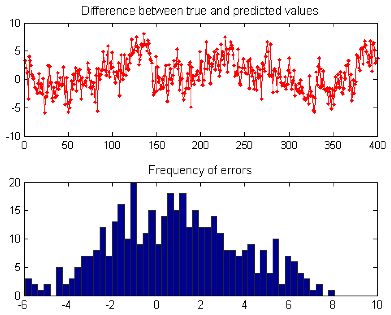
Furthermore, Figure 3 shows the performance of the model on the test set. The upper subplot illustrates the prediction error, and the lower subplot depicts the error frequency. It can be seen from Figure 3 that the prediction error of the model is concentrated between −6 °C and 6 °C, with an RMSE of 3.0186 and the corresponding MAPE of 5.5088. Overall, the ESN model performs well on the test data.

In order to achieve status monitoring, the EWMA method was adopted to calculate the upper and lower bounds of pitch motor temperature. Figure 4 shows the experimental results of the test set. In addition, the corresponding EWMA warning lines were also plotted, in which the red and green curves represent the upper and lower warning bounds, respectively. Notice that the wind turbine is in a normal state on the test data set, hence there is no alarm, and the experimental results are consistent with the expectation.

In order to test how well the ESN model works for the early warning of pitch motor faults, some data of the No. 1 wind turbine containing pitch motor faults were utilized. In the recorded data, a pitch motor fault occurred at 3:50 a.m. on 5 August 2013. In this specific experiment, we selected 8000 records before the fault, that is, the data from 7 June 2013 to 3 August 2013, as the training data, and tested whether the fault can be predicted.

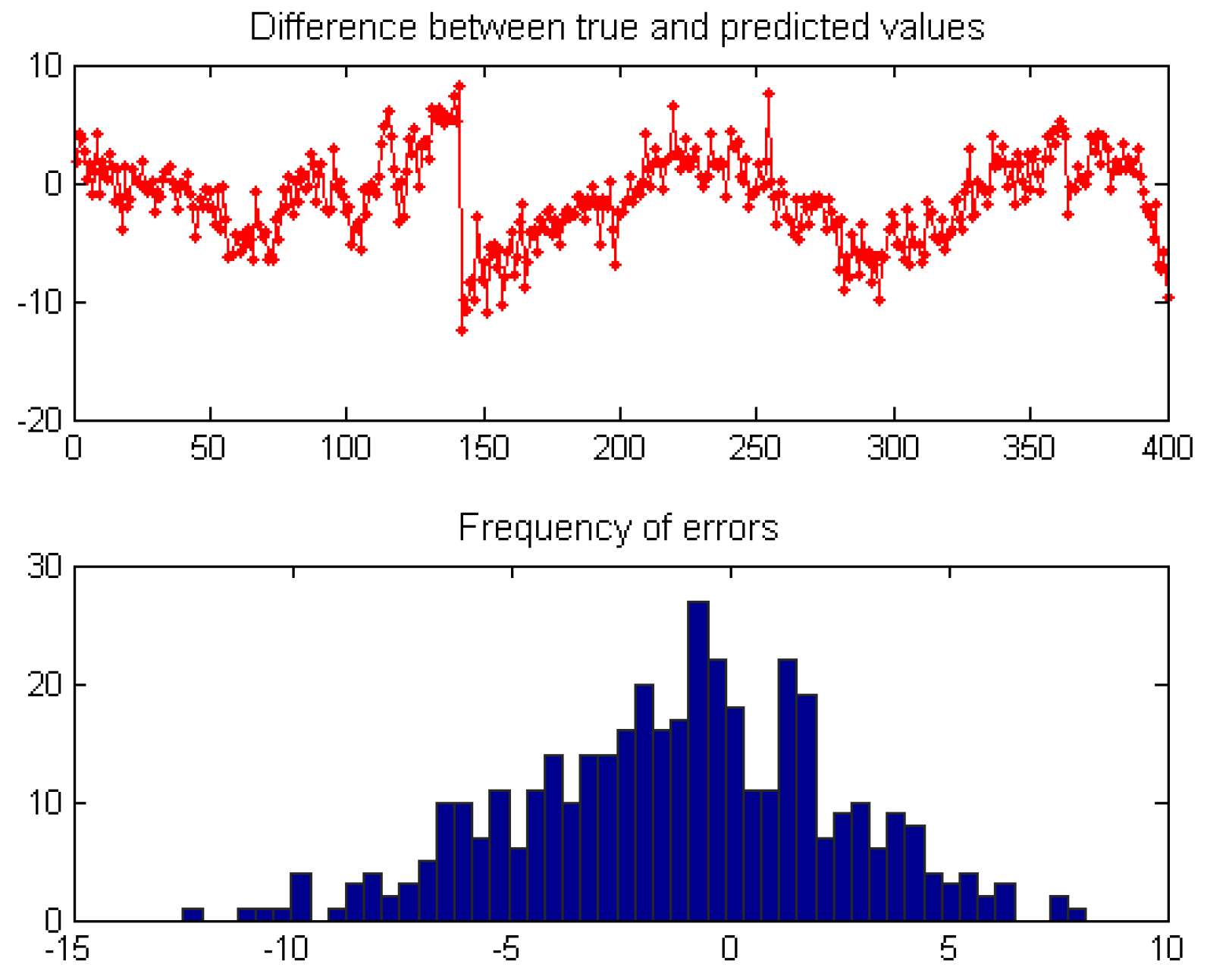
Figure 5 shows the true and predicted values on the training set as well as the prediction error. Similarly, the x-axis represents the time index and the y-axis denotes the pitch motor temperature. The training data are all generated during the normal operation of the turbine. It can be seen from Figure 5 that the prediction error is basically between −10 °C and 10 °C.

Figure 6 shows the predicted results of the trained ESN model on the test set. Here, the prediction error and error frequency histograms are shown. It can be observed that the prediction error range of the model is similar to that of the training set, and most of the errors lie between −5 °C and 5 °C.

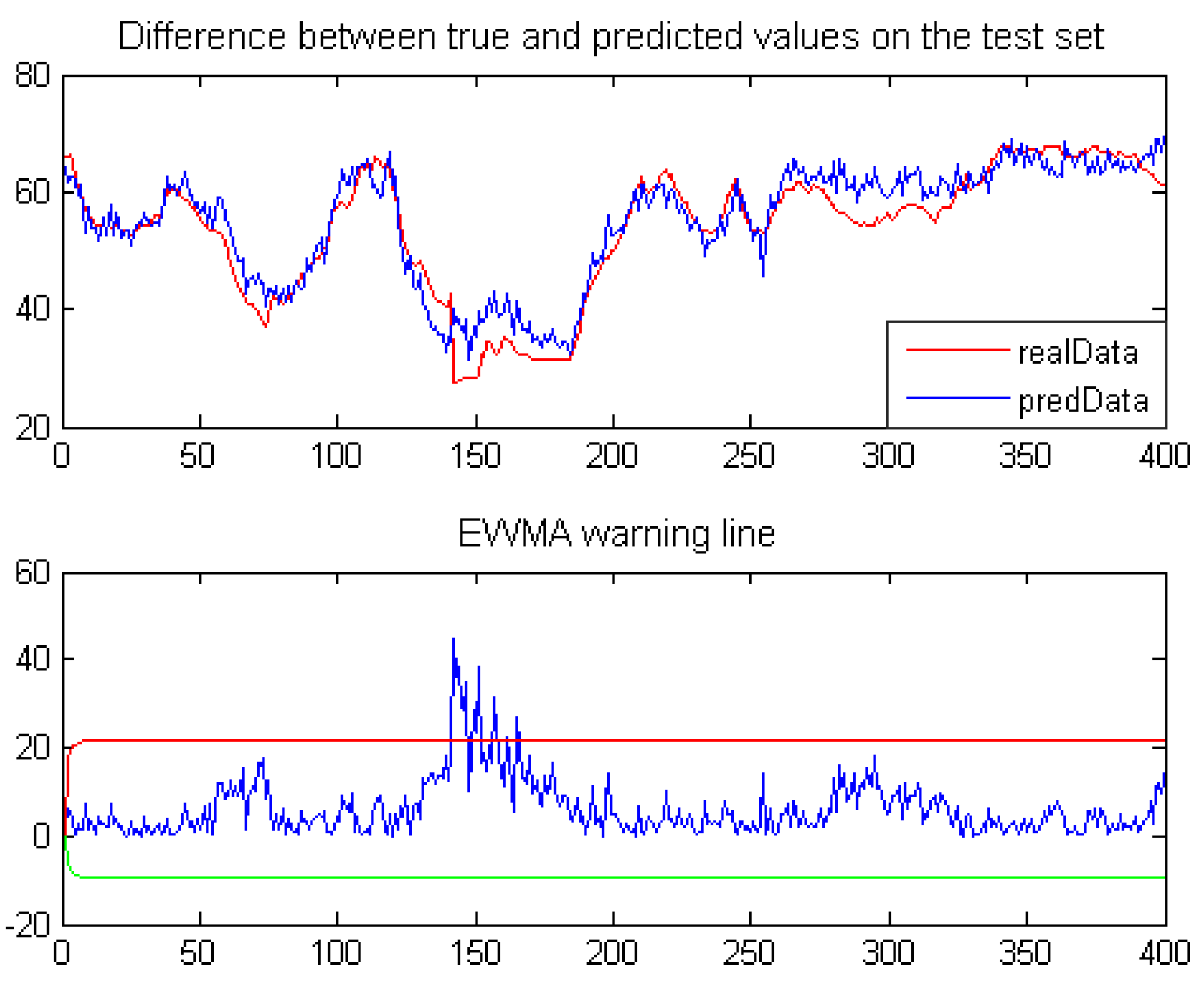
Since there is a fault record in the test set at this time, the purpose of ESN is to detect the occurrence of the fault point in advance. Figure 7 displays the true and predicted values on the test set as well as the EWMA fault warning diagram corresponding to the ESN model. We can see that ESN can detect the occurrence of the fault because its APE exceeds the upper warning limit. Notice that the real fault occurred at 3:50 on 5 August 2013 (please note the places corresponding to the points between 140 to 150 in Figure 7). When ESN predicted the data at 3:10, the corresponding APE exceeds the upper warning bound, and the warning information appears. This means that the ESN model successfully identifies the sudden change of the turbine operation state 40 min in advance. The above experiments show that the ESN-based normal behavior model is effective for early warning of pitch motor faults.

5. Conclusions and Future Work

Based on the normal behavior model, this paper studies the status monitoring of the pitch motor in an electronic motor. Considering that the state of the motor varies with time, the SCADA data are used to train an echo state network to predict the temperature of the pitch motor. Then, the residual analysis technology is used to detect the sudden changes in its running state. Particularly, the EWMA technique is used to set the alarm limit lines of each parameter. The experimental results show that this method can effectively identify and provide an early warning about the faults of the pitch motor.

As for the status monitoring problem of the pitch motor, one of its core ingredients is a time series prediction task. In recent years, some advanced deep neural networks such as LSTM (long-and-short term memory) [21], temporal convolutional networks [22] and the transformer model [23] have exhibited excellent performance on this type of forecasting task since they can more effectively capture the long-term effect of input features to the target variable. Thus, it will be interesting to investigate how well they will perform in solving the tasks of status monitoring and early warning. We will pursue this in one of our near future works.

References

1. McMillan, D.; Ault, G.W. Condition monitoring benefit for onshore wind turbines: Sensitivity to operational parameters. IET Renew. Power Gener. 2008, 2, 60–72. [Google Scholar] [CrossRef]
2. Chehouri, A.; Younes, R.; Ilinca, A.; Perron, J. Review of performance optimization techniques applied to wind turbines. Appl. Energy 2015, 142, 361–388. [Google Scholar] [CrossRef]
3. Yang, W.; Court, R.; Jiang, J. Wind turbine condition monitoring by the approach of SCADA data analysis. Renew. Energy 2013, 53, 365–376. [Google Scholar] [CrossRef]
4. Schlechtingen, M.; Santos, I.F. Comparative analysis of neural network and regression based condition monitoring approaches for wind turbine fault detection. Mech. Syst. Signal Processing 2011, 25, 1849–1875. [Google Scholar] [CrossRef] [Green Version]
5. Wang, Y.; Infield, D. Supervisory control and data acquisition data-based non-linear state estimation technique for wind turbine gearbox condition monitoring. IET Renew. Power Gener. 2013, 7, 350–358. [Google Scholar] [CrossRef]
6. Zhang, Z.Y.; Wang, K.S. Wind turbine fault detection based on SCADA data analysis using ANN. Adv. Manuf. 2014, 2, 70–78. [Google Scholar] [CrossRef] [Green Version]
7. Sun, P.; Li, J.; Wang, C.; Lei, X. A generalized model for wind turbine anomaly identification based on SCADA data. Appl. Energy 2016, 168, 550–567. [Google Scholar] [CrossRef] [Green Version]
8. Schlechtingen, M.; Santos, I.F.; Achiche, S. Wind turbine condition monitoring based on SCADA data using normal behavior models. Part 1: System description. Appl. Soft Comput. 2013, 13, 259–270. [Google Scholar] [CrossRef]
9. Schlechtingen, M.; Santos, I.F. Wind turbine condition monitoring based on SCADA data using normal behavior models. Part 2: Application examples. Appl. Soft Comput. 2014, 14, 447–460. [Google Scholar] [CrossRef]
10. Wang, L.; Zhang, Z.; Long, H.; Xu, J.; Liu, R. Wind turbine gearbox failure identification with deep neural networks. IEEE Trans. Ind. Inform. 2016, 13, 1360–1368. [Google Scholar] [CrossRef]
11. Srivastava, N.; Hinton, G.; Krizhevsky, A.; Sutskever, I.; Salakhutdinov, R. Dropout: A simple way to prevent neural networks from overfitting. J. Mach. Learn. Res. 2014, 15, 1929–1958. [Google Scholar]
12. Gulbudak, O.; Gokdag, M. Predictive dual-induction machine control using nine-switch inverter for multi-drive systems. In Proceedings of the IEEE 12th International Conference on Compatibility, Power Electronics and Power Engineering (CPE-POWERENG), Doha, Qatar, 10–12 April 2018; pp. 1–6. [Google Scholar]
13. Gulbudak, O.; Santi, E. A predictive control scheme for a dual output indirect matrix converter. In Proceedings of the IEEE Applied Power Electronics Conference and Exposition (APEC), Charlotte, NC, USA, 15–19 March 2015; pp. 2828–2834. [Google Scholar]
14. Sun, C.; Sun, D.; Zheng, Z.; Nian, H. Simplified Model Predictive Control for Dual Inverter-Fed Open-Winding Permanent Magnet Synchronous Motor. IEEE Trans. Energy Convers. 2018, 33, 1846–1854. [Google Scholar] [CrossRef]
15. Lukoševičius, M. A practical guide to applying echo state networks. In Neural Networks: Tricks of the Trade; Springer: Berlin/Heidelberg, Germany, 2012; pp. 659–686. [Google Scholar]
16. Jaeger, H. The “echo state” approach to analysing and training recurrent neural networks. Bonn Ger. Ger. Natl. Res. Cent. Inf. Technol. GMD Tech. Rep. 2001, 148, 13. [Google Scholar]
17. Jang, J.S.R. ANFIS: Adaptive-network-based fuzzy inference system. IEEE Trans. Syst. Man Cybern. 1993, 23, 665–685. [Google Scholar] [CrossRef]
18. Nielsen, M. Neural Networks and Deep Learning; Determination Press: San Francisco, CA, USA, 2018. [Google Scholar]
19. Goodfellow, I.; Bengio, Y.; Courville, A. Deep Learning; MIT Press: Cambridge, MA, USA, 2016. [Google Scholar]
20. Crowder, S.V.; Vander Wiel, S.A. Exponentially Weighted Moving Average (EWMA) Control Chart. In Wiley StatsRef: Statistics Reference Online; Balakrishnan, N., Colton, T., Everitt, B., Piegorsch, W., Ruggeri, F., Teugels, J.L., Eds.; Wiley: Hoboken, NJ, USA, 2014; Available online: https://onlinelibrary.wiley.com/doi/10.1002/9781118445112.stat04041 (accessed on 14 June 2022).
21. Yu, Y.; Si, X.; Hu, C.; Zhang, X. A review of recurrent neural networks: LSTM cells and network architecture. Neural Comput. 2019, 31, 1235–1270. [Google Scholar] [CrossRef] [PubMed]
22. Bai, S.; Kolter, J.Z.; Koltun, V. An empirical evaluation of generic convolutional and recurrent networks for sequence modeling. arXiv 2018, arXiv:1803.01271. [Google Scholar]
23. Vaswani, A.; Shazeer, N.; Parmar, N.; Uszkoreit, J.; Jones, L.; Gomez, A.N.; Kaiser, Ł.; Polosukhin, I. Attention is all you need. In Proceedings of the Advances in Neural Information Processing Systems 30 (NIPS 2017), Long Beach, CA, USA, 4–9 December 2017; Volume 30, pp. 5998–6008. [Google Scholar]
Figure 1. The architecture of an echo state network.
Applsci 12 07747 g001
Figure 2. Prediction of pitch motor temperature by ESN model on training data set.
Applsci 12 07747 g002
Figure 3. Temperature prediction error of pitch motor on test set.
Applsci 12 07747 g003
Figure 4. Early warning of models on test set.
Applsci 12 07747 g004
Figure 5. Prediction of ESN model on training set.
Applsci 12 07747 g005
Figure 6. Prediction error of pitch motor temperature test set.
Applsci 12 07747 g006
Figure 7. Pitch motor fault early warning.
Applsci 12 07747 g007