A New Solving Method Based on Simulated Annealing Particle Swarm Optimization for the Forward Kinematic Problem of the Stewart–Gough Platform

Abstract

The forward kinematics of the Stewart–Gough platform is vital for high-precision positioning and sensing in six degrees of freedom. In this paper, the solving of forward kinematics is converted to searching for the best posture corresponding to the input outrigger length vectors by inverse kinematic calculation. The simulated annealing (SA) process is embedded into particle swarm optimization (PSO) to improve the convergence speed and overcome the local convergence. The proposed SA–PSO algorithm not only accelerates the convergence speed but also improves the reliability and success rate. After the optimization of algorithm parameters, the success rate of the SA–PSO for random outrigger length vector input is steadily above 99.9% while the results of PSO is between 93% and 100%. In the workspace simulation, the average iteration number of the proposed algorithm is reduced from 146.6 to 122.7, meanwhile, the success rate of SA–PSO is 99.992%, much higher than the 93.805% of PSO. Compared with the traditional Newton–Raphson method, the SA–PSO method has a higher success rate and is less time consuming. Finally, a physical experiment is conducted on a six-degree-of-freedom platform, revealing that the given algorithm is reliable and accurate.

1. Introduction

Since its invention by Gough and Stewart [1], the six-degrees-of-freedom (six DOF) parallel platform has rapidly become popular because of its high stiffness, accuracy, and strong bearing capacity. Nowadays, the Stewart–Gough platform (SGP) is widely applied to motion simulation, optical precision machining, intelligent medical treatment, aerospace positioning, and space measurement. The forward kinematic problem (FKP) of the platform refers to predicting the posture in six degrees of freedom by the length of the six outriggers. The FKP is of great significance for posture detection, SGP calibrating, and high-precision positioning. However, the FKP mathematically means multivariate higher-order nonlinear equations, from which it is a big challenge to ascertain the unique solution.

In order to obtain the high-precision forward solution and improve real-time applications, researchers have put forward many ideas. B. Mourrain and P. Dietmaier found 40 forward solutions by algebraic method [2,3]. M. Raghavan et al. analyzed the polynomial solution of forward kinematics for the different parallel platform [4,5]. Tae-Yong Lee et al. applied the algebraic method to choose one out of all possible postures [6,7]. A. Nag et al. proposed a kind of generic geometric–algebraic framework for FKP [8]. These above algebraic methods analyze the FKP as a math problem, which cannot be applied in engineering, therefore, numerical methods have attracted the attention of researchers. The Newton–Raphson (NR) method is popular for seeking the solutions of nonlinear equations because of its simplicity and fast convergence. Watkins and Chi fu Yang put forward a global NR method to avoid the divergence caused by the selection of initial value [9,10]. However, the NR method requires calculation of the Jacobi matrix or Hessian matrix, which may not exist in some situations, and the calculation of partial derivatives is not conducive to real-time application. Kilryong Han et al. analyzed the number of extra sensors for the FKP of different SGP configurations [11]. Vincenzo Parenti-Castelli et al. made use of two extra rotary sensors to help achieve the solution, and their method could reduce the computational burden [12]. By optimizing the sensor installation position, Yu-Jen Chiu and Ming-Hwei Perng proposed a method based on three redundant sensors, and this method is insensitive to the sensor position deviation and measurement error [13]. By adding additional sensors, the calculation can be simplified. However, the measurement system will increase the costs and the measurement error introduced is also a big challenge. With the improvement of computing power, many intelligent methods have been applied to the calculation of robot kinematics. Pratik J. Parikh, Sarah S. Lam and Choon seng Yee both trained a neural network to replace tedious kinematic calculation [14,15]. Zhelong Wang et al. analyzed the SGP by using the principal component analysis [16]. In this way, the FKP was converted to a two-dimensional nonlinear minimization problem. Antonio Morell et al. developed a popular machine learning method—support vector machines—for classification and regression, and they finally built a solution model for the FKP [17]. However, these intelligent algorithms require a large number of prior data, which are not scalable and are inconvenient to apply to practical engineering.

In this paper, two vector spaces are built: one is composed of all possible length vectors, which is called space L, and the other, named space Q, is filled with posture vectors. The FKP now is regarded as mapping space L to space Q through the complex nonlinear relationship. Considering efficiency and accuracy, the PSO method combined with the SA process is raised to find the target posture from space Q. In Section 2, the geometric structure and kinematics of SGP are analyzed in detail. Section 3 redefines the FKP problem from the perspective of spatial mapping, and the SA–PSO method is introduced to deal with it. The comparative simulation experiments including repetitive, continuous trajectory, and workspace random tests are carried out in Section 4, which verify that the proposed SA–PSO method performs better than standard PSO and NR method. The SA–PSO method is also validated by physical verification in Section 4, and the results of experiment show the effectiveness and reliability of the given method. Section 5 is the conclusion.

2. Kinematics Analysis

2.1. Configuration and Coordinate System of SGP

According to different connection modes of upper and lower hinge points, the configuration of SGP can be divided into 6-6 (six upper jungles and six lower jungles), 6-3 (six upper jungles and three lower jungles), and 3-3 (three upper jungles and three lower jungles). In this paper, the classical structure of the 6-6 form is used as the research object. It is worth mentioned that the idea proposed in this paper is also applicable to other configurations of parallel platforms. As shown in Figure 1a, 6-6 SGP consists of top platform A, base platform B, and six actuator outriggers which are respectively linked to the top and base platforms by twelve upper and lower hinges.

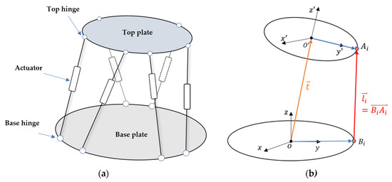
Figure 1. Simplified structure and vector geometry diagram of the SGP. (a) Main components of SGP. (b) Kinematic vector diagram of single outrigger.

Given a moving coordinate system $o^{\prime }{x}^{\prime }{y}^{\prime }{z}^{\prime }$, $o^{\prime }$ is the center of the top plate, ${\mathit{A}}_i$ is the center of top hinge i (Figure 1b). The global coordinate system $oxyz$ describes the base plate, $o$ is the center of the base plate, ${\mathit{B}}_i$ is the center of the base hinge i. The posture of the top plate is composed of position vector $\left(x,y,z\right)$ and rotation vector $\left(\alpha ,\beta ,\gamma \right)$. The points described in the moving coordinate can be transformed to the global coordinate by rotation operator $\mathit{R}\left(\alpha ,\beta ,\gamma \right)$ and translation operator $\mathit{L}\left(x,y,z\right)$.

2.2. Inverse Kinematic Analysis

With the posture $\mathit{q}=\left(x,y,z,\alpha ,\beta ,\gamma \right)$ of the moving plate, the length vector of the six outriggers $\mathit{l}=\left(l_1,l_2,l_3,l_4,l_5,l_6\right)$ can be calculated $\stackrel{\rightharpoonup }{{\mathit{l}}_{\mathit{i}}}$ = $\stackrel{\rightharpoonup }{{\mathit{B}}_{\mathit{i}}{\mathit{A}}_{\mathit{i}}}$, so the vector relationship of outriggers can be described as follows:

$$\stackrel{\rightharpoonup }{{\mathit{B}}_{\mathit{i}}{\mathit{A}}_{\mathit{i}}}=\stackrel{\rightharpoonup }{\mathit{O}{\mathit{O}}^{\prime }}+\stackrel{\rightharpoonup }{{\mathit{O}}^{\prime }{\mathit{A}}_{\mathit{i}}}-\stackrel{\rightharpoonup }{\mathit{O}{\mathit{B}}_{\mathit{i}}}$$

(1)

Which is:

$$\stackrel{\rightharpoonup }{ {\mathit{l}}_{\mathit{i}}}=\stackrel{\rightharpoonup }{{\mathit{t}}_{\mathit{i}}}+\mathit{R}\stackrel{\rightharpoonup }{{\mathit{A}}_{\mathit{i}}}-\stackrel{\rightharpoonup }{\mathit{O}{\mathit{B}}_{\mathit{i}}}$$

(2)

where:

$$\mathit{R}=\left[\begin{array}{ccc}cos\gamma cos\beta & cos\gamma sin\beta sin\alpha -sin\gamma cos\alpha & sin \gamma sin \alpha +cos\gamma sin\beta cos\alpha \\ sin\gamma cos\beta & cos\alpha cos\gamma +sin\gamma sin\beta sin\alpha & sin\gamma sin\beta cin\alpha -cos\gamma sin\alpha \\ -sin\beta & cos\beta sin\alpha & cos\beta cos\alpha \end{array}\right]$$

R is z-y-x Euler transformation matrix, $\stackrel{\rightharpoonup }{{\mathit{t}}_{\mathit{i}}}=\left(x,y,z\right)$ is the position vector of the top platform

Let:

$${\mathit{P}}_{\mathit{i}}=\mathit{R}\stackrel{\rightharpoonup }{{\mathit{A}}_{\mathit{i}}}$$

So, the length of the six outriggers is

$$\begin{gathered} {\mathit{l}}_{\mathit{i}}=\sqrt{{\displaystyle {\displaystyle \sum }_{k=1}^3}{\left[{\mathit{P}}_{\mathit{i}}\left(k\right)-{\mathit{B}}_{\mathit{i}}\left(k\right)\right]}^2} \\ i=1, 2, 3\dots 6 \end{gathered}$$

(3)

(3) is the inverse kinematic solution formula of outrigger length. Obviously, it is easy and fast for computer to calculate the length of six outriggers corresponding to the given posture by solving (3).

2.3. Forward Kinematic Problem

In practical terms, it is hard to directly measure the motion posture of the moving platform in six degrees of freedom. Therefore, an efficient and high-accuracy forward solution algorithm is of great significance for the real-time estimation and detection of motion platform posture, which is critical for high precision positioning.

Contrary to the inverse kinematic problem, the forward kinematics focuses on finding the unknown posture $\left(x,y,z,\alpha ,\beta ,\gamma \right)$ from the given six leg length $\left(l_1,l_2,l_3,l_4,l_5,l_6\right)$. The multivariate nonlinear equations which describe the forward kinematics are as follows.

$$f_i\left(x,y,z,\alpha ,\beta ,\gamma \right)=l_i-\sqrt{{\left(t_i+R{A}_i-O{B}_i\right)}^T\left(t_i+R{A}_i-O{B}_i\right)}=0$$

(4)

i = 1, 2, 3 … 6

These six multivariate nonlinear equations describe the forward kinematics of the SGP and the posture can be gotten by solving them which is also a complex problem.

2.4. Newton–Raphson Method for FKP

The Newton–Raphson method is a traditional numerical method to solve multivariate nonlinear equations. It turns the nonlinear equations to linear equations through Taylor formula expansion, and gradually gains on the solution of the equations through continuous iteration of approximate solutions. The Jacobian matrix of nonlinear equations is

$$J\left(X^k\right)=\frac{\partial \left(F(X^k\right)}{\partial X^k}$$

(5)

When $J$ is reversible, te root formula is:

$$X^{k+1}=X^k-J{\left(X^k\right)}^{-1}F\left(X^k\right)$$

(6)

The steps of Newton–Raphson method to numerically solve the nonlinear equations are as follows:

(1)

Set the initial value $X^0$, maximum iterations N, and the target accuracy $\epsilon$. Set k = 0.

(2)

Solve $d^k=-J{\left(X^k\right)}^{-1}F\left(X^k\right)$.

(3)

If $\left|d^k\right|<\epsilon$, stop the iteration, or set $X^{k+1}=X^k+d^k$.

(4)

If k = N, stop the iteration, or set k = k + 1, turn to (2).

An important condition of using Newton–Raphson method is that the Jacobian matrix of nonlinear equations at the operating point exists and the matrix shall be nonsingular. Moreover, the computation of the Jacobian matrix and its inverse is complex. This method’s convergences rely on the selection of initial values, while the inappropriate selection of initial values will make the solving progress difficult to converge.

3. SA–PSO Method for FKP

Through the above analysis, it can be concluded that the FKP problem of SGP is much more complex than the IKP. Because of the complexity of the nonlinear equations, it is hard to attain the unique forward solution by the math analytical method. To make it easy to understand, space Q and space L are separated for the IKP and FKP (Figure 2). We can rethink this question in another way: it is easy to determine whether a posture is an accurate solution of (5). The FKP problem can be remodeled as finding a suitable way to conveniently find a posture $\mathit{q}$ in the workspace to satisfy (5). Then, the problem of solving nonlinear equations has become a problem of searching for an optimal solution.

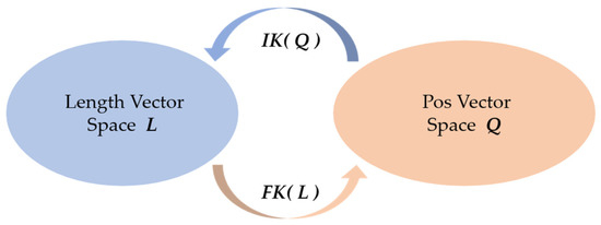
Figure 2. Space Q and L are linked by IK( ) and FK( ).

3.1. Particle Swarm Optimization

The problem is how to find the right $\mathit{q}$ in an efficient way since there are endless $\mathit{q}$ vectors in space Q. PSO is a heuristic evolutionary calculation method, derived from the study of bird predation behavior [18]. The main idea of PSO is to search for the optimal solution through cooperation and information sharing among the group.

In PSO, each particle represents a solution to the target problem with two important attributes: velocity $\mathit{v}$ and position $\mathit{x}$. Each particle searches for the optimal solution separately in the target space and it marks its position as the extreme ${\mathit{P}}_{\mathit{b}\mathit{e}\mathit{s}\mathit{t}}$ of the current individual. The optimal solution ${\mathit{G}}_{\mathit{b}\mathit{e}\mathit{s}\mathit{t}}$ of the whole generation of PSO is picked from the individual extremums. In the k + 1th iteration, the position and velocity of particle i is updated by:

$$\begin{gathered} {{\mathit{x}}_{\mathit{i}}}^{\mathit{k}+1}={\mathit{x}}_{\mathit{i}}{}^{\mathit{k}}+{\mathit{v}}_{\mathit{i}}{}^{\mathit{k}+1} \\ {\mathit{v}}_{\mathit{i}}{}^{\mathit{k}+1}=\omega {\mathit{v}}_{\mathit{i}}{}^{\mathit{k}}+c_{1}rand\left({\mathit{P}}^{\mathit{k}}{}_{\mathit{b}\mathit{e}\mathit{s}\mathit{t},\mathit{i}}-{\mathit{x}}_{\mathit{i}}{}^{\mathit{k}}\right)+c_{2}rand\left({\mathit{G}}^{\mathit{k}}{}_{\mathit{b}\mathit{e}\mathit{s}\mathit{t}}-{\mathit{x}}_{\mathit{i}}{}^{\mathit{k}}\right) \end{gathered}$$

(7)

where: $\omega$ is inertia coefficient, the larger the ω, the better the global search performance; $c_1 c_2$ are learning factors. $rand$ is a random number range from 0 to 1. ${\mathit{P}}^{\mathit{k}}{}_{\mathit{b}\mathit{e}\mathit{s}\mathit{t},\mathit{i}}$ is the best value of particle i in the kth iteration while ${\mathit{G}}^{\mathit{k}}{}_{\mathit{b}\mathit{e}\mathit{s}\mathit{t}}$ is the global best value in the kth iteration.

3.2. Improvement by Simulated Annealing Process

One shortcoming of PSO is that particles may appear premature, then the algorithm traps them into the local optimum. The result of local optimum is that the algorithm cannot find the optimal solution meeting the accuracy requirements. The SA algorithm is derived from the principle of solid annealing and has the ability to jump out of the local optimal trap [19]. The main idea of the SA is that the optimization problem is simulated by a thermodynamic system, the energy of the system is regarded as the objective function of the optimization problem, and the optimization process is simulated by the annealing process of gradually cooling the system to reach the lowest energy state. The SA algorithm has the ability of probability jump in the search process, and can effectively avoid the search process trapping into a local minimum. It has been proven theoretically that the SA algorithm converges to the global optimal solution with a probability of 1 under certain conditions [20].

To avoid the local optimum, the SA algorithm is integrated into the selection of ${\mathit{P}}_{\mathit{b}\mathit{e}\mathit{s}\mathit{t}}$ of PSO to improve the ability to jump out of the local minimum. For the proposed SA–PSO method, ${\mathit{P}}_{\mathit{b}\mathit{e}\mathit{s}\mathit{t}}{}_{\mathit{i}}^{\mathit{k}+1}$ is individual optimum of particle $\mathit{i}$ in the $\mathit{k}+1$ iteration, and it is updated by:

$${\mathit{P}}_{\mathit{b}\mathit{e}\mathit{s}\mathit{t}}{}_{\mathit{i}}^{\mathit{k}+\mathbf{1}}=\{\begin{array}{c}{\mathit{x}}_{\mathit{i}}^{\mathit{k}+1}, fi{t}^{k+1}<fi{t}^k or Pr{o}^{k+1}>rand \\ {\mathit{P}}_{\mathit{b}\mathit{e}\mathit{s}\mathit{t}}{}_{\mathit{i}}^{\mathit{k}}, fi{t}^{k+1}>fi{t}^k and Pr{o}^{k+1}<rand\end{array}$$

(8)

While:

• $fi{t}^k: \mathrm{the} \mathrm{fitness} \mathrm{of} \mathrm{the} {\mathit{P}}_{\mathit{b}\mathit{e}\mathit{s}\mathit{t}}{}_{\mathit{i}}^{\mathit{k}}$
• $fi{t}^{k+1}: \mathrm{the} \mathrm{fitness} \mathrm{of} \mathrm{the} {\mathit{x}}_{\mathit{i}}^{\mathit{k}+\mathbf{1}}$
• $Pr{o}^{k+1}: \mathrm{the} \mathrm{SA} \mathrm{probability} \mathrm{for} \mathrm{the} k+1 \mathrm{iteration}$
• $rand: \mathrm{random} \mathrm{number} \mathrm{range} \mathrm{from} 0 \mathrm{to} 1$

The individual optimum is allowed to receive the non-minimum by a probability of $Pr{o}^{k+1}$,which makes the particles search the SA neighborhood. This kind of SA randomness can jump out of the local minimum. The important factor $Pr{o}^{k+1}$ conforms to Boltzmann distribution and it is calculated by:

$$\begin{array}{c}Pr{o}^{k+1}=e^{-fi{t}^{k+1}/T^{k+1}}\\ T^{k+1}={\kappa }_B{T}^k\end{array}$$

(9)

While:

• $T^{k+1}: \mathrm{the} \mathrm{annealing} \mathrm{temperature} \mathrm{of} \mathrm{the} k+1 \mathrm{iteration}$
• $T^k: \mathrm{the} \mathrm{annealing} \mathrm{temperature} \mathrm{of} \mathrm{the} k \mathrm{iteration}$
• ${\kappa }_B: \mathrm{the} \mathrm{Boltzmann} \mathrm{constant}$

The initial temperature $T^0$ depends on the complexity of the problem. Here, we calculated it with the fitness of the initial population: $T^0=∆fitness\ast population size$. $∆fitness$ is the maximum difference in the fitness. As is shown in Figure 3, the SA searching increased the randomness and received non-optimal individual optimum. In this way, the SA neighborhood searching can help the PSO algorithm jump out of the local optimum.

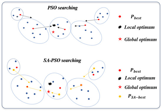
Figure 3. The searching progress comparison of PSO and SA–PSO.

3.3. Fitness Function for the FKP Problem of SA–PSO

Considering the one-to-one correspondence between each vector in space Q and space L, the indicator is set as the Euclidean distance of the difference vector between ${\mathit{l}}_{\mathit{S}\mathit{A}-\mathit{P}\mathit{S}\mathit{O}}$ and ${\mathit{l}}_{\mathbf{0}}$ (${\mathit{l}}_{\mathit{S}\mathit{A}-\mathit{P}\mathit{S}\mathit{O}}$is the length vector of q which is found by SA–PSO, ${\mathit{l}}_{\mathbf{0}}$ is the given length vector), while (10) describes the indicator. When the indicator meets the accuracy requirements, the solution is considered to be generally obtained. More importantly, the Euclidean distance fitness can be regarded as a sign of the success of optimization.

$$fit=\sqrt{{\displaystyle \sum }_{i=1}^6{\left({\mathit{l}}_{\mathit{S}\mathit{A}-\mathit{P}\mathit{S}\mathit{O}}\left(i\right)-{\mathit{l}}_{\mathbf{0}}\left(i\right)\right)}^2/6}$$

(10)

where:

$${\mathit{l}}_{\mathit{S}\mathit{A}-\mathit{P}\mathit{S}\mathit{O}}=IK\left(\mathit{q}\right)$$

Notes: $IK( )$ is the inverse kinematic function.

3.4. SA–PSO Algorithm

The SA–PSO algorithm is introduced by the following Algorithm 1. The difference between the standard PSO and SA–PSO is the selection of the individual optimum.

Algorithm 1: Simulated Annealing Particle Swarm Optimization (SA–PSO) for FKP.

Input: Length of outriggers $\mathit{l}$, Accuracy $\mathit{\epsilon }$, PSO parameters: (Population size $\mathit{N}$, Dimension $\mathit{D}$, Learning factors ${\mathit{c}}_{\mathbf{1}} {\mathit{c}}_{\mathbf{2}}$, Maximum number of iterations ${\mathit{K}}_{\mathit{m}\mathit{a}\mathit{x}}$, Weight limit ${\mathit{w}}_{\mathit{m}\mathit{a}\mathit{x}}, {\mathit{w}}_{\mathit{m}\mathit{i}\mathit{n}}$, Position limit ${\mathit{x}}_{\mathit{m}\mathit{a}\mathit{x}}, {\mathit{x}}_{\mathit{m}\mathit{i}\mathit{n}}$, Velocity limit ${\mathit{v}}_{\mathit{m}\mathit{a}\mathit{x}}, {\mathit{v}}_{\mathit{m}\mathit{i}\mathit{n}}$), Boltzmann constant ${\mathit{\kappa }}_{\mathit{B}}$.

Output: Predicted posture $\mathit{q}=\left(x_{trans},y_{trans},z_{trans},x_{rot},y_{rot},z_{rot}\right)$.

1: For each particle $i$

2: Initialize the position ${\mathit{x}}_{\mathit{i}}{}^{\mathbf{0}}$ the velocity ${\mathit{v}}_{\mathit{i}}{}^{\mathbf{0}}$ with the permissible range

3: End for

4: For each particle i

5: Calculate the fitness value $fi{t}_i^0=IK\left({\mathit{x}}_{\mathit{i}}^{\mathbf{0}}\right)$

6: Initialize the individual optimum and fitness ${\mathit{P}}_{\mathit{i},\mathit{b}\mathit{e}\mathit{s}\mathit{t}}^{\mathbf{0}}={\mathit{x}}_{\mathit{i}}^{\mathbf{0}},P\_fi{t}_i^0=fi{t}_i^0$

7: End for

8: Initialize the global optimum ${\mathit{G}}_{\mathit{b}\mathit{e}\mathit{s}\mathit{t}}^0={\mathit{x}}_{\mathit{j}}^{\mathbf{0}} (j=index(\min \left(fi{t}^0\right)$) $G\_fi{t}^0=fi{t}^0$

9: Iteration $k=1$

10: Do

11: Calculate the weight by $w^k=w_{max}-k\left(w_{max}-w_{min}\right)/K_{max}$

12: For each particle i

13: Calculate velocity ${\mathit{v}}_{\mathit{i}}^{\mathit{k}}$

14: Update particle position

15: Calculate the fitness $fi{t}_i^k=IK\left({\mathit{x}}_{\mathit{i}}^{\mathit{k}}\right)$

16: End for

17: For each particle i

18: Find the individual best optimum ${\mathit{P}}_{\mathit{i},\mathit{b}\mathit{e}\mathit{s}\mathit{t}}^{\mathit{k}}$and update the $P\_fi{t}_i^k$

19: End for

20: Update the global optimum of iteration $k$:

21: ${\mathit{G}}_{\mathit{b}\mathit{e}\mathit{s}\mathit{t}}^{\mathit{k}}={\mathit{x}}_{\mathit{j}}^{\mathit{k}} (j=index(\min \left(P\_fi{t}^k\right)$) $G\_fi{t}^k=P\_fi{t}_j^k$

22: Annealing: $T^k={\kappa }_B{T}^{k-1}$

23: $k=k+1$

24: While the $G\_fi{t}^k<\epsilon$ or $k=K_{max}$

25: Output: the predicted posture $\mathit{q}$ is ${\mathit{G}}_{\mathit{b}\mathit{e}\mathit{s}\mathit{t}}$

4. Simulation and Physical Experiments

The distribution of platform hinge points is shown in Figure 4, the origin $o^{\prime }$ of the moving coordinate system is located at the center of the upper surface of the top platform, and the origin $o$ of the global coordinate system is located at the center of the circle where the center point of the lower hinge is. Due to the symmetry of the SGP structure, the following parameters are enough to define the platform: radius $\mathit{r}$ and $\mathit{R}$ of top and base circumscribed circle of hinge point, the angle between adjacent hinge points ${\mathit{\theta }}_{\mathbf{1}}$ and ${\mathit{\theta }}_{\mathbf{2}}$ and distance ${\mathit{h}}_{\mathbf{1}}$, ${\mathit{h}}_{\mathbf{2}}$ from upper and lower hinge points to the top platform surface. The SGP can be uniquely determined by the above six parameters. The parameters of the top and base platform for simulation are set as follows:

$$r=0.2 \mathrm{m}, R=0.3 \mathrm{m}, h_1=0.05 \mathrm{m},h_2=0.3 \mathrm{m},{\theta }_1={\theta }_2=\frac{\pi }{6} rad$$

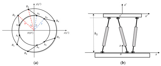
Figure 4. The geometry and parameters of the SGP. (a) The vertical view of the platform. (b) The main view of the platform.

Table 1 shows the coordinates of the hinge points, while the top coordinates are based on the moving coordinate system, and the base coordinates are described in the global coordinate system.

Table 1. The coordinates of the SGP hinge points for simulation (unit: centimeter).

Top	Coordinates (cm)	Base	Coordinates (cm)
${\mathit{A}}_{\mathbf{1}}$	[−19.3185, −5.1764, −5]T	${\mathit{B}}_{\mathbf{1}}$	[−21.2132, −21.2132, 0]T
${\mathit{A}}_{\mathbf{2}}$	[−19.3185, 5.1764, −5]T	${\mathit{B}}_{\mathbf{2}}$	[−21.2132, 21.2132, 0]T
${\mathit{A}}_{\mathbf{3}}$	[5.1764, 19.3185, −5]T	${\mathit{B}}_{\mathbf{3}}$	[−7.7646, 28.9778, 0]T
${\mathit{A}}_{\mathbf{4}}$	[14.1421, 14.1421, 5]T	${\mathit{B}}_{\mathbf{4}}$	[28.9778, 7.7664, 0]T
${\mathit{A}}_{\mathbf{5}}$	[14.1421, −14.1421, −5]T	${\mathit{B}}_{\mathbf{5}}$	[28.9778, −7.7664, 0]T
${\mathit{A}}_{\mathbf{6}}$	[5.1764, −19.3185, −5]T	${\mathit{B}}_{\mathbf{6}}$	[−7.7664, −28.9778, 0]T

With the points in Table 1, the initial outrigger length ${\mathit{l}}_{\mathbf{0}}$ is calculate by IK function.

$${\mathit{l}}_{\mathbf{0}}=29.7619\times {10}^{-2} \mathrm{m}$$

4.1. Optimiazation of SA–PSO Parameters

On the premise of ensuring the success rate, the parameters of SA–PSO algorithm are optimized to reduce the solution time [21]. A set of relatively optimal parameters in Table 2 are obtained. It should be mentioned that all the simulation experiments in the following are carried out in the MATLAB R2021b and the computer CPU is Ryzen 7-5800H.

Table 2. SA–PSO parameters after optimization.

Parameter	Value	Parameter	Value
Population	80	${\kappa }_B$	0.98
$w_{max}$	0.42	$w_{min}$	$0.1$
$c_1$	1.8	$c_2$	2.2
$x_{min},x_{max}$	$\pm 0.3$ m or rad	$v_{min},v_{max}$	$\pm 0.03$ m or rad

The PSO parameters are almost the same as SAPSO method without the annealing progress. Considering the convergence speed and accuracy, the weight value decreases with iteration from 0.42 to 0.1. The range of workspace decides the position range, and the range of particles are usually 10% of the position range. The most important parameters are maximum of iterations and the size of population. The optimal parameters are found one by one.

4.2. Feasibility Simulation of SAPSO

The feasibility simulation experiment is designed as follows:

(1)

Given the posture value $\mathit{q}$of the top platform. (To be solved)

(2)

Calculate the $\mathit{l}$length vector of the six outriggers corresponding to $\mathit{q}$ by IK function. (Input)

(3)

Send $\mathit{l}$ to the SA–PSO algorithm, find the optimal solution ${\mathit{q}}_{SA-PSO}$ (solving).

The SA–PSO algorithm parameters for FKP are set as Table 2. The target posture $\mathit{q}$ is q1 = 0.1208 m, q2 = 0.1009 m, q3 = 0.0817 m, q4 = 0.1824 rad, q5 = 0.0634 rad, q6 = 0.1504 rad.

While the corresponding $\mathit{l}$ is calculated by $IK( )$

l1 = 0.3581 m, l2 = 0.3202 m, l3 = 0.3643 m, l4 = 0.3394 m, l5 = 0.2358 m, l6 = 0.4126 m. The value of six dimensions is obtained by the SA–PSO algorithm, and the convergence of each dimension is shown in Figure 5. When the iteration reaches 113 times, the target accuracy is almost achieved. Table 3 gives the final error of each dimension of the posture and the error of each dimension finally converges to the corresponding accuracy.

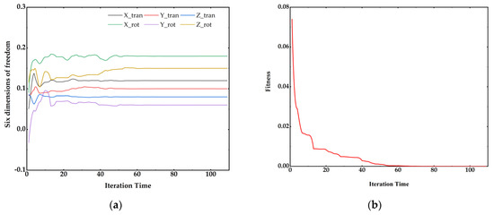
Figure 5. Convergence of Six–DOF and fitness by SA–PSO method. (a) Posture convergence progress with iteration. (b) Fitness convergence with iteration.

Table 3. Error of each dimension by SA–PSO.

Dimension	$\mathbf{Error} \left({\mathbf{10}}^{-\mathbf{7}}\right)$	Dimension	$\mathbf{Error} \left({\mathbf{10}}^{-\mathbf{7}}\right)$
X-trans	0.0133	X-rot	−0.1810
Y-trans	0.0660	Y-rot	0.3021
Z-trans	−0.0122	Z-rot	−0.0730

The dimension error is a little larger than the Euclidean distance fitness accuracy $\mathit{\epsilon }$, which is based on the structure of SGP. The following simulation is to analyze the relationship between fitness accuracy and iterations. Run the proposed SA–PSO algorithm 10,000 times, count average iterations and record the running time of each solving for different accuracy. It can be seen from Table 4, in order to achieve higher dimension accuracy, the fitness accuracy $\mathit{\epsilon }$ will be higher, which means the iteration time will increase.

Table 4. Average iterations and time for different accuracy.

$\mathbf{Accuracy} \mathit{\epsilon }$	$\mathbf{Average} \mathbf{Iterations} {\mathit{K}}_{\mathit{e}\mathit{v}}$
${10}^{-6}$	95.61
${10}^{-7}$	107.10
${10}^{-8}$	117.54
${10}^{-9}$	127.16
${10}^{-10}$	135.94

4.3. Reliability Simulation

The above analysis and experiments prove the feasibility of the SA–PSO algorithm in the FKP problem of SGP. However, in practical application, the algorithm must have both high precision and low computing time. Moreover, the robustness of the algorithm is also vital. The six DOF postures of SGP change continuously, the proposed SA–PSO algorithm must adapt to it.

4.3.1. Success Rate Comparison

To verify the repeatability and compare the success rate of the PSO and SA–PSO method, six groups of repeated simulation experiments are designed as follows. The target postures are randomly generated in the reachable workspace, and each group carries out the FKP solving 10,000 times. The accuracy is set as ${10}^{-8}$.

By the comparison of PSO and SA–PSO, as is shown in Table 5, the addition of simulated annealing steps improves the success rate of the FKP solving, while reducing the number of iterations and accelerating the convergence of the algorithm. For the ${10}^{-8}$ accuracy, the performance of the SA–PSO algorithm is much more stable with a success rate above 99.90%, while the average iterations are less than 120. While the standard PSO method has a lower convergence speed with no less than 140 iterations, and it has a lower and unstable success rate. For random input of $\mathit{q}$ values, the SA–PSO method has better robustness than the PSO method.

Table 5. The average number of iterations and success rate.

Group	PSO		SA–PSO
	${\mathit{k}}_{\mathit{e}\mathit{v}}$	Success Rate	${\mathit{k}}_{\mathit{e}\mathit{v}}$	Success Rate
1	146.36	94.54%	116.07	99.92%
2	140.81	100%	113.51	100%
3	144.56	95.91%	113.51	99.96%
4	140.53	100%	112.61	100%
5	142.83	96.23%	114.88	99.97%
6	142.10	95.47%	114.00	99.99%
7	144.54	98.49%	115.11	99.93%
8	140.55	100%	112.45	100%
9	147.17	94.28%	115.00	99.96%
10	148.02	93.89%	114.12	100%

4.3.2. Continuous Motion Trajectory Simulation

Continuous motion trajectory is set to test the robustness of PSO and SA–PSO. As shown in Table 6, the complex motion of SGP is composed of six sets of postures and each set is a single degree of the motion. Two seconds are cut out and the sampling rate is 1 kHz. Then two thousand posture points are solved into two thousand length vectors by inverse kinematic function, then the vector series are passed to the algorithms. Figure 6 shows the six degrees motion and the moving trajectory of six outriggers.

Table 6. The six-dimensional trajectory.

Posture	Dimension	Motion Trajectory
$\mathit{X-trans}$	$Q_1\left(t\right)$	$0.15\sin \left(2\mathsf{\pi }\mathrm{t}\right)$
$\mathit{Y-trans}$	$Q_2\left(t\right)$	$0.12\sin \left(2\mathsf{\pi }\mathrm{t}\right)$
$\mathit{Z-trans}$	$Q_3\left(t\right)$	$0.1t$
$\mathit{X-rot}$	$Q_4\left(t\right)$	$0.10\sin \left(\mathsf{\pi }\mathrm{t}\right)$
$\mathit{Y-rot}$	$Q_5\left(t\right)$	$0.20\sin \left(\mathsf{\pi }\mathrm{t}\right)$
$\mathit{Z-rot}$	$Q_6\left(t\right)$	$0.05\sin \left(\mathsf{\pi }\mathrm{t}\right)$

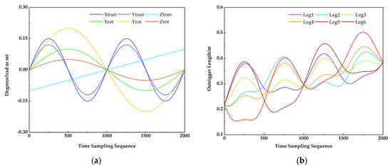
Figure 6. Continuous motion of the platform. (a) Motion of six degrees. (b) Length of six outriggers.

Figure 7 shows the simulation results of PSO and SA–PSO algorithm, both of them achieve the given accuracy ${10}^{-8}$ in continuous posture motion. While the progress of each time solving is described by Figure 8 and Table 7. The proposed SA–PSO algorithm has fewer average iterations and smaller standard deviation than the PSO algorithm which verifies that the former has higher efficiency and better stability than the latter.

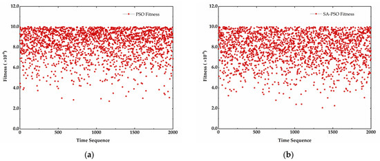
Figure 7. The fitness for the continuous trajectory. (a) Fitness of PSO. (b) Fitness of SA–PSO.

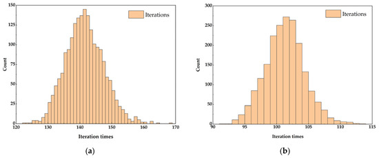
Figure 8. The histogram of iterations for the continuous trajectory. (a) Iterations of PSO. (b) Iterations of SA–PSO.

Table 7. The comparison between PSO and SA–PSO in iterations.

Items	PSO	SA–PSO
Average iterations	141.00	100.82
Maximum iterations	168	113
Minimum iterations	122	91
Standard deviation	5.98	3.10

4.3.3. Whole Workspace Randomly Simulation

In this section, 100,000 postures are generated randomly and evenly in workspace ${\mathit{Q}}_{work}$. Find the corresponding outriggers length space ${\mathit{L}}_{work}$ by $IK\left(Q_{work}\right)$, pass ${\mathit{L}}_{work}$ to the two algorithms, and find the solving results. Figure 9 illustrates the comparison between PSO and SA–PSO. The success rate of SA–PSO is 99.992% with only eight group points trapped into the local convergence. However, the PSO method only reaches 93.805% with 6195 groups error solving. The average iterations are 122.7256 versus 146.6126, and the SA–PSO algorithm shows its fast convergence speed than PSO. The success rate and iterations verify the robustness and feasibility of the proposed algorithm in the whole workspace.

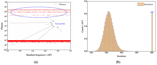
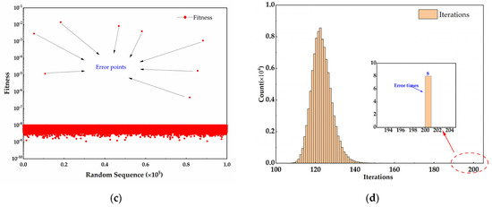
Figure 9. The fitness results and the iterations of the whole workspace postures. (a) Fitness of PSO soling results for workspace sampling. (b) Histogram of PSO iterations. (c) Fitness of SA–PSO solving results for workspace sampling. (d) Histogram of SA–PSO iterations.

4.4. Comparison between NR Method and SAPSO

In this section, we compare the success rate and the time consuming between the NR method and the SA–PSO algorithm. Five groups of experiments are designed. Each group solves 1000 randomly generated L points. The target accuracy is set as ${10}^{-8}$. The solving results are illustrated in Table 8.

Table 8. The random comparison experiments between NR and SA–PSO.

Test	Success Rate (%)		Average Time Consuming (s)
	NR	SA–PSO	NR	SA–PSO
1	96.2	99.9	0.3708	0.0372
2	97.4	100	0.3468	0.0356
3	97.7	99.8	0.3725	0.0377
4	97.3	100	0.4706	0.0348
5	97	100	0.3638	0.0350

The NR method fails in some points when the initial value is set as [0 0 0 0 0 0], which may be not proper for these points. When the iteration of NR method is active, it no longer converges. However, because of the randomness introduced to the optimization progress, the SAPSO can work well in these points. Moreover, the SA–PSO method is more efficient than NR method with the operation time less than 40 milliseconds, almost 10% of the NR method.

4.5. Physical Verification Experiments

To demonstrate the applicability of the SA–PSO method, experiments are carried on the Stewart–Gough platform H-850 with six laser displacement sensors calculating the length change of six outriggers. The experimental platform is shown in Figure 10. The measurement accuracy of the laser displacement sensor is $10 \mathsf{\mu }\mathrm{m}$, and its measuring range is $\pm 5 \mathrm{mm}$. The hexapod platform can be controlled by a moving signal from the controller, and the parameters of it are illustrated in Table 9.

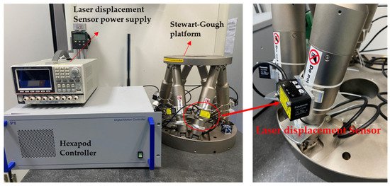
Figure 10. The experimental platform to verify the SA–PSO forward solution.

Table 9. The coordinates of the joints of the Stewart–Gough platform H-850.

Top	Coordinate (mm)	Base	Coordinate (mm)
${\mathit{A}}_{\mathbf{1}}$	${\left[-90.9842,-22.7693,-29.9670\right]}^T$	${\mathit{B}}_{\mathbf{1}}$	${\left[-90.6333,-116.3188,-273.0900\right]}^T$
${\mathit{A}}_{\mathbf{2}}$	${\left[-90.9842, 22.7693,-29.9670\right]}^T$	${\mathit{B}}_{\mathbf{2}}$	${\left[-90.6333, 116.3188,-273.0900\right]}^T$
${\mathit{A}}_{\mathbf{3}}$	${\left[25.7733, 90.1793,-29.9670\right]}^T$	${\mathit{B}}_{\mathbf{3}}$	${\left[-55.4184, 136.6501,-273.0900\right]}^T$
${\mathit{A}}_{\mathbf{4}}$	${\left[65.2109,67.4100,-29.9670\right]}^T$	${\mathit{B}}_{\mathbf{4}}$	${\left[146.0517, 20.3313,-273.0900\right]}^T$
${\mathit{A}}_{\mathbf{5}}$	${\left[65.2109,-67.4100,-29.9670\right]}^T$	${\mathit{B}}_{\mathbf{5}}$	${\left[146.0517,-20.3313,-273.0900\right]}^T$
${\mathit{A}}_{\mathbf{6}}$	${\left[25.7733,-90.1793,-29.9670\right]}^T$	${\mathit{B}}_{\mathbf{6}}$	${\left[-55.4184,-136.6501,-273.0900\right]}^T$

Let the H-850 Stewart–Gough platform move in a single degree of freedom, record the reading of the laser displacement sensor, pass it to the SA–PSO forward kinematic algorithm, and finally compare the errors between the algorithm results and the given motion postures of the platform.

The experimental results show that the SA–PSO algorithm can accurately calculate the corresponding platform posture value through the input outrigger length. In Figure 11, the errors between the solution results and the given posture of the controller are no more than$40 \mathsf{\mu }\mathrm{m}$. The main sources of these errors are as follows: 1, the measurement error of the laser displacement sensor; and 2, the positioning error of the platform itself. The measurement accuracy of the laser displacement sensor is not more than 10 $\mathsf{\mu }\mathrm{m}$, and the structure error caused by the installation will also reduce the accuracy of outrigger rod length measurement. There will be a small positioning deviation when the platform moves. In the future, precise optical means can be used to calibrate the attitude of the platform. Based on the efficiency of the SA–PSO algorithm in forward kinematics, we will next consider applying the algorithm to the model calibration of the SGP structure.

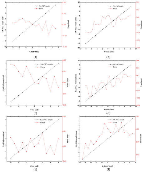
Figure 11. The SA–PSO results and the error for the experiments. (a) X rotation results and errors. (b) X translation results and errors. (c) Y rotation results and errors. (d) Y translation results and errors. (e) Z rotation results and errors. (f) Z translation results and errors.

5. Conclusions

Forward kinematic solution is meaningful and vital for the building and analysis of the Stewart–Gough platform. In this paper, the link between the length of six outriggers and posture in six dimensions is built by the proposed optimum algorithm. Through the calculation of the inverse kinematic solution and optimum of the input posture, the result gradually converges to the target solution. To overcome the disadvantage of the standard PSO method, a simulated annealing method is applied to the PSO method to help the algorithm remove the local optimum. The feasibility simulation shows that the SA–PSO is a good method for solving the forward kinematics. Based on this, a group of simulations with different accuracy levels is carried out. And the results indicate the method works well for high accuracy with more iterations. Also, the improved algorithm performs better than the standard PSO method in repetitive simulation experiments with higher success rate and faster convergence speed. The continuous trajectory simulation and the workspace random simulation further verify the better reliability and the superior robustness of the proposed algorithm. As for the convergence dilemma of NR method in some special points, the SA–PSO method performs better than the traditional numerical algorithm in success rate and real-time application, that means it is a powerful complement to traditional algorithms. Finally, a physical platform is built to test the proposed SA–PSO method. It is concluded that for the Stewart–Gough platform, the accurate prediction of posture is based on the precise model of the structure, efficient forward kinematic solving, and high precision measurement of six outriggers. Furthermore, it is significative to study the application of this algorithm in platform design, assembly, parameter calibration and motion control in the future.

References

- Stewart, D. A Platform with Six Degrees of Freedom. In Proceedings of the Institution of Mechanical Engineers, London, UK, 1 June 1965; Volume 180, pp. 371–386. [Google Scholar]
- Mourrain, B. The 40 “generic” positions of a parallel robot. In Proceedings of the 1993 International Symposium on Symbolic and Algebraic Computation, Kiev, Ukraine, 6–8 July 1993; pp. 173–182. [Google Scholar] [CrossRef]
- Dietmaier, P. The Stewart-Gough Platform of General Geometry can have 40 Real Postures. In Advances in Robot Kinematics: Analysis and Control; Springer: Dordrecht, The Netherlands, 1998; pp. 7–16. [Google Scholar] [CrossRef]
- Raghavan, M.; Roth, B. Solving Polynomial Systems for the Kinematic Analysis and Synthesis of Mechanisms and Robot Manipulators. J. Mech. Des. 1995, 117, 71–79. [Google Scholar] [CrossRef]
- Husty, M. An algorithm for solving the direct kinematics of general Stewart-Gough platforms. Mech. Mach. Theory 1996, 31, 365–379. [Google Scholar] [CrossRef]
- Lee, T.-Y.; Shim, J.-K. Forward kinematics of the general 6–6 Stewart platform using algebraic elimination. Mech. Mach. Theory 2001, 36, 1073–1085. [Google Scholar] [CrossRef]
- Lee, T.-Y.; Shim, J.-K. Improved dialytic elimination algorithm for the forward kinematics of the general Stewart–Gough platform. Mech. Mach. Theory 2003, 38, 563–577. [Google Scholar] [CrossRef]
- Nag, A.; Safar, V.; Bandyopadhyay, S. A uniform geometric-algebraic framework for the forward kinematic analysis of 6-6 Stewart platform manipulators of various architectures and other related 6-6 spatial manipulators. Mech. Mach. Theory 2020, 155, 104090. [Google Scholar] [CrossRef]
- Kelley, C.T. Solving Nonlinear Equations with Newton’s Method; Society for Industrial and Applied Mathematics: Philadelphia, PA, USA, 2003. [Google Scholar]
- Yang, C.-F.; Zheng, S.-T.; Jin, J.; Zhu, S.-B.; Han, J.-W. Forward kinematics analysis of parallel manipulator using modified global Newton-Raphson method. J. Cent. South Univ. Technol. 2010, 17, 1264–1270. [Google Scholar] [CrossRef]
- Han, K.; Chung, W.; Youm, Y. New Resolution Scheme of the Forward Kinematics of Parallel Manipulators Using Extra Sensors. J. Mech. Des. 1996, 118, 214–219. [Google Scholar] [CrossRef]
- Parenti-Castelli, V.; Di Gregorio, R. A New Algorithm Based on Two Extra-Sensors for Real-Time Computation of the Actual Configuration of the Generalized Stewart-Gough Manipulator. J. Mech. Des. 1999, 122, 294–298. [Google Scholar] [CrossRef]
- Chiu, Y.-J.; Perng, M.-H. Forward Kinematics of a General Fully Parallel Manipulator with Auxiliary Sensors. Int. J. Robot. Res. 2001, 20, 401–414. [Google Scholar] [CrossRef]
- Parikh, P.J.; Lam, S.S. Solving the forward kinematics problem in parallel manipulators using an iterative artificial neural network strategy. Int. J. Adv. Manuf. Technol. 2008, 40, 595–606. [Google Scholar] [CrossRef]
- Yee, C.S.; Lim, K.-B. Forward kinematics solution of Stewart platform using neural networks. Neurocomputing 1997, 16, 333–349. [Google Scholar] [CrossRef]
- Wang, Z.; He, J.; Shang, H.; Gu, H. Forward kinematics analysis of a six-DOF Stewart platform using PCA and NM algorithm. Ind. Robot. Int. J. Robot. Res. Appl. 2009, 36, 448–460. [Google Scholar] [CrossRef] [Green Version]
- Morell, A.; Tarokh, M.; Acosta, L. Solving the forward kinematics problem in parallel robots using Support Vector Regression. Eng. Appl. Artif. Intell. 2013, 26, 1698–1706. [Google Scholar] [CrossRef]
- Eberhart, R.; Kennedy, J. A new optimizer using particle swarm theory. In Proceedings of the Sixth International Symposium on Micro Machine and Human Science, Nagoya, Japan, 4–6 October 1995; pp. 39–43. [Google Scholar] [CrossRef]
- Van Laarhoven, P.J.M.; Aarts, E.H.L. Simulated annealing. In Simulated Annealing: Theory and Applications; Springer: Berlin/Heidelberg, Germany, 1987; pp. 7–15. [Google Scholar]
- Rutenbar, R. Simulated annealing algorithms: An overview. IEEE Circuits Dev. Mag. 1989, 5, 19–26. [Google Scholar] [CrossRef]
- Shieh, H.-L.; Kuo, C.-C.; Chiang, C.-M. Modified particle swarm optimization algorithm with simulated annealing behavior and its numerical verification. Appl. Math. Comput. 2011, 218, 4365–4383. [Google Scholar] [CrossRef]
Publisher’s Note: MDPI stays neutral with regard to jurisdictional claims in published maps and institutional affiliations. |
© 2022 by the authors. Licensee MDPI, Basel, Switzerland. This article is an open access article distributed under the terms and conditions of the Creative Commons Attribution (CC BY) license (https://creativecommons.org/licenses/by/4.0/).