1. Introduction
Autonomous and stand-alone solutions that can work together are becoming increasingly popular in automation and robotics [
1,
2]. This makes it possible to build a fault-tolerant unit, which can act independently of a powerful main server and allows for reducing the amount of data transmitted over the network. The goal can be achieved by putting some data processing mechanisms in peripheral units [
3], such as microcontrollers. The advantages of this approach are (1) the insensitivity to server malfunction and (2) the high availability rate. Unfortunately, it may result in poor output quality, e.g., of sensor value estimations, because of the generally lower performance of a unit, and the limited hardware resources. The situation may be even more difficult if a sophisticated algorithm, such as a particle filter (PF) [
4], is used, which produces a high-quality output but requires a more powerful processing unit compared to other estimation algorithms [
5]. Higher output quality means a better match to the real-life signal value, which is desirable.
In a case where the measurement data needs to be improved, or it is necessary to determine the values of non-measurable variables, state estimation is desirable. Formerly, thanks to the low computational complexity, static estimation, such as weighted least squares (WLS) [
6], was mainly used in automation. Unfortunately, low computational complexity was accompanied by low estimation quality. With the development and increased capabilities of computing devices, dynamic state estimation approaches have become widely used. One of the most popular methods for linear systems was the Kalman filter (KF) [
7,
8], proposed by Rudolf Kalman in 1960 [
9]. Later, many variants of Kalman filters for estimating a state of nonlinear systems were proposed. The most common modifications are: based on static linearization, the extended Kalman filter (EKF) [
10], and, based on the unscented transformation, the unscented Kalman filter (UKF) [
11]. Other interesting modifications can be found in [
12,
13,
14,
15]. A more complex algorithm, but also of better output quality for highly nonlinear objects, is the particle filter (PF), proposed in 1993 by Gordon, Salmond, and Smith [
4]. It is based on the randomization of particles and the calculation of their weights best matching the system’s actual output. Over the years, various types of particle filters have been developed, such as an auxiliary particle filter (APF) [
16] or a likelihood particle filter (LPF) [
17]. The main differences involve selecting the transition function from which the particles are drawn. The particle filter is extremely useful in scenarios where enough processing power is available. In previous works, the authors proposed a modification relating to the parallelization of the basic particle filter, dividing it into smaller parts—the sub-filters. The code can be efficiently parallelized [
18], resulting in a reduction of processing time without a negative impact on the output quality (except for the resampling step, which is very important in PF methods and, unfortunately, cannot be parallelized).
Problems of applying the efficient use of microcontrollers and PF together have been analyzed in several works [
19,
20,
21]. The researchers used a variety of platforms, ranging from hardware to software. The researchers used different types of platforms, which varied at the hardware and software levels. Some of them were built on commercial hardware platforms offered by, e.g., LEGO Mindstorms. The common parts of the above-mentioned platforms are a high-performance processor and a large amount of RAM memory. The platforms based on low-cost boards such as Nucleo and Discovery boards from ST, Arduino family boards, or just ESP8266 are rare. That was the motivation to test one of the mentioned platforms and check its performance. In our case, we decided to get an older platform—the results can be easily improved by simply replacing the board with its newer equivalent.
The main subject of research in this publication is the state estimation in the temperature control system. The object was prepared as a dedicated platform for this research. In the literature, there are examples of the use of state estimation of thermal processes. For example, in [
22], a particle filter was used to regulate the temperature, with the proposed adjustment of particle weights to improve the operation of the algorithm. The authors rely on a complex non-linear process model. In [
23], the authors experimentally determined the parameters of the temperature control model, both in an open- and closed-loop system. However, the model was based only on measurement information—the development of the research may be the use of state estimation to improve this information. One can find many sources on the use of temperature estimation for various devices. In works [
24,
25], the new temperature estimation technique in a permanent magnet using Kalman filtering is proposed. The article [
26] presents a review of various methods of state estimation in battery modeling tasks, using the state of temperature too.
In this paper, emphasis is put on the implementation of PF on a computationally weak device; therefore, a simplified (linear) model is adopted concerning [
22]. Such an approach provides better implementation options and the opportunity to increase the number of particles. Various versions of the mathematical model that have been proposed can be successfully used for state estimation.
The structure of the work is as follows.
Section 2 describes the particle filter algorithm.
Section 3 contains the description of the computing platform.
Section 4 describes the control object and the procedure of how to identify it.
Section 5 describes the results of the experiments.
Section 6 and
Section 7 contain the discussion and summary, respectively.
2. Particle Filter
The particle filter is a state estimation algorithm that can be used on linear or nonlinear discrete-time systems, including systems with non-Gaussian noises. The system is represented by the following equations:
where
k denotes the time step number,
is the state vector,
is the control inputs vector,
is the vector of measurement outputs,
is the transition functions vector, and
is the measurement functions vector,
and
are the process and measurement noises, respectively. The transition and measurement model can be linear or nonlinear. In the latter case, the equations of state cannot be written in a matrix form [
27].
The main purpose of the state estimation is to obtain internal variables that cannot be directly measured and to filter out measurement noise from the signals .
The basis of the particle filter is the recursive Bayesian filter algorithm [
28,
29]
where:
—the set of output vectors,
—the posterior Probability Density Function (PDF);
—the likelihood;
—the prior PDF;
—the evidence which is given by equation
The posterior PDF in the particle filter is represented by a set of particles, and its weights are given by
, where each particle
has a weight
, for
. The approximation of posterior PDF for a large number of particles can be written as
where
denotes a Dirac Delta function.
The first proposed particle filter algorithm is the bootstrap algorithm [
4,
28] presented in Algorithm 1 and in
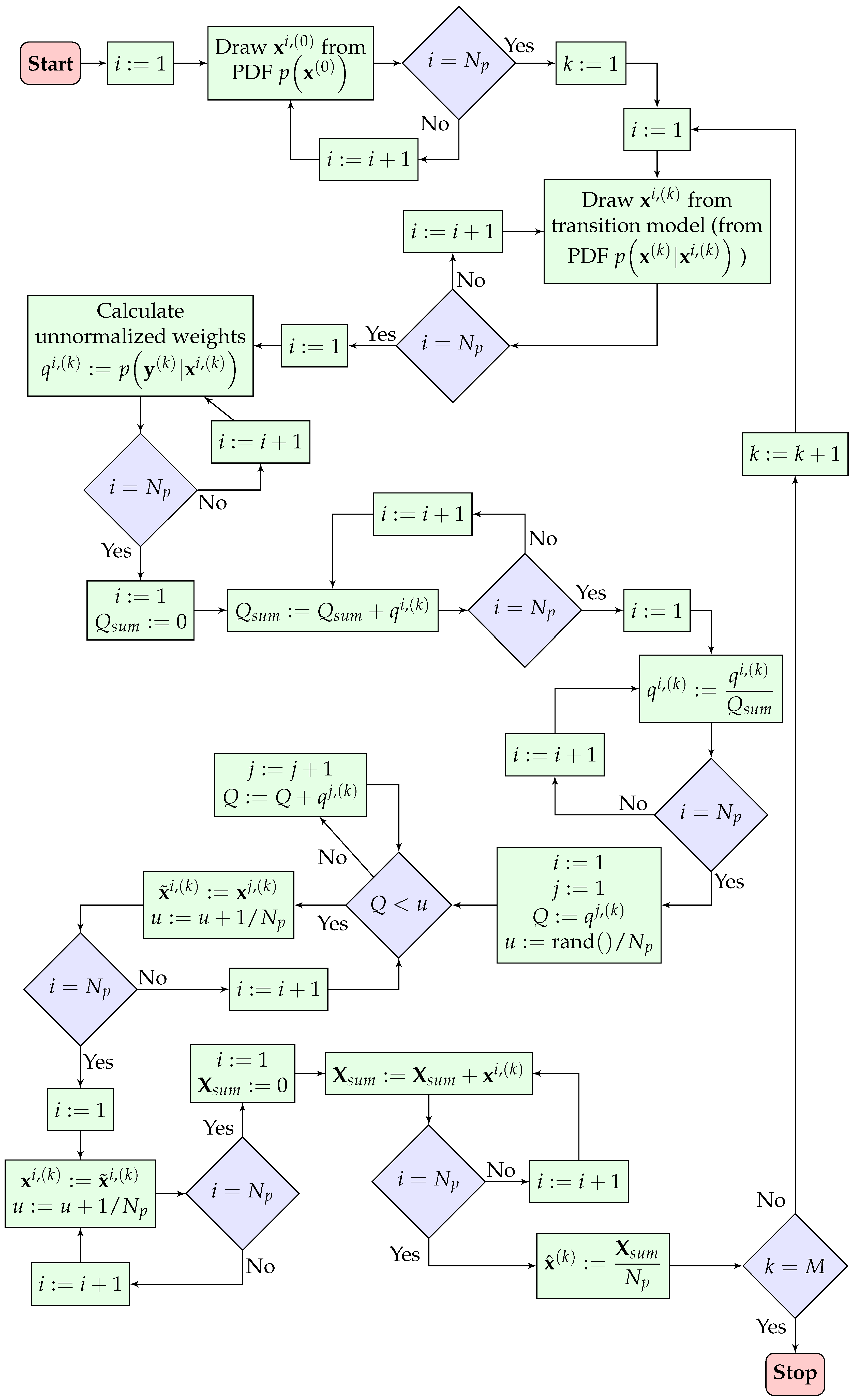
Figure 1.
| Algorithm 1: Bootstrap Particle Filter (BPF) |
| 1. Initialization. Draw initial values from the posterior PDF . Set time step . Do this step only once.
|
| 2. Prediction. Draw the new particles , where from the transition model.
|
| 3. Update. Determine the weights of the particles based on the measurement model
|
| 4. Normalization. Scale values of the weights in such a way that their sum equals 1.
|
| 5. Resampling. Draw particles from among those that already exist. The PDF for drawing is defined by the set of normalized weights (the systematic resampling is applied [30]).
|
| 6. End of the iteration. Estimate the state vector at k-th time step, increase the time step . Jump to the 2nd step.
|
3. The Platform
Our tests were carried out on a temperature control system, prepared as a dedicated platform built of commercially available elements. The platform consists of three related parts:
A case—made of steel, plexiglass, printable elements;
Hardware—microcontroller, sensors, H-bridge, and others;
Software—code written in the C programming language.
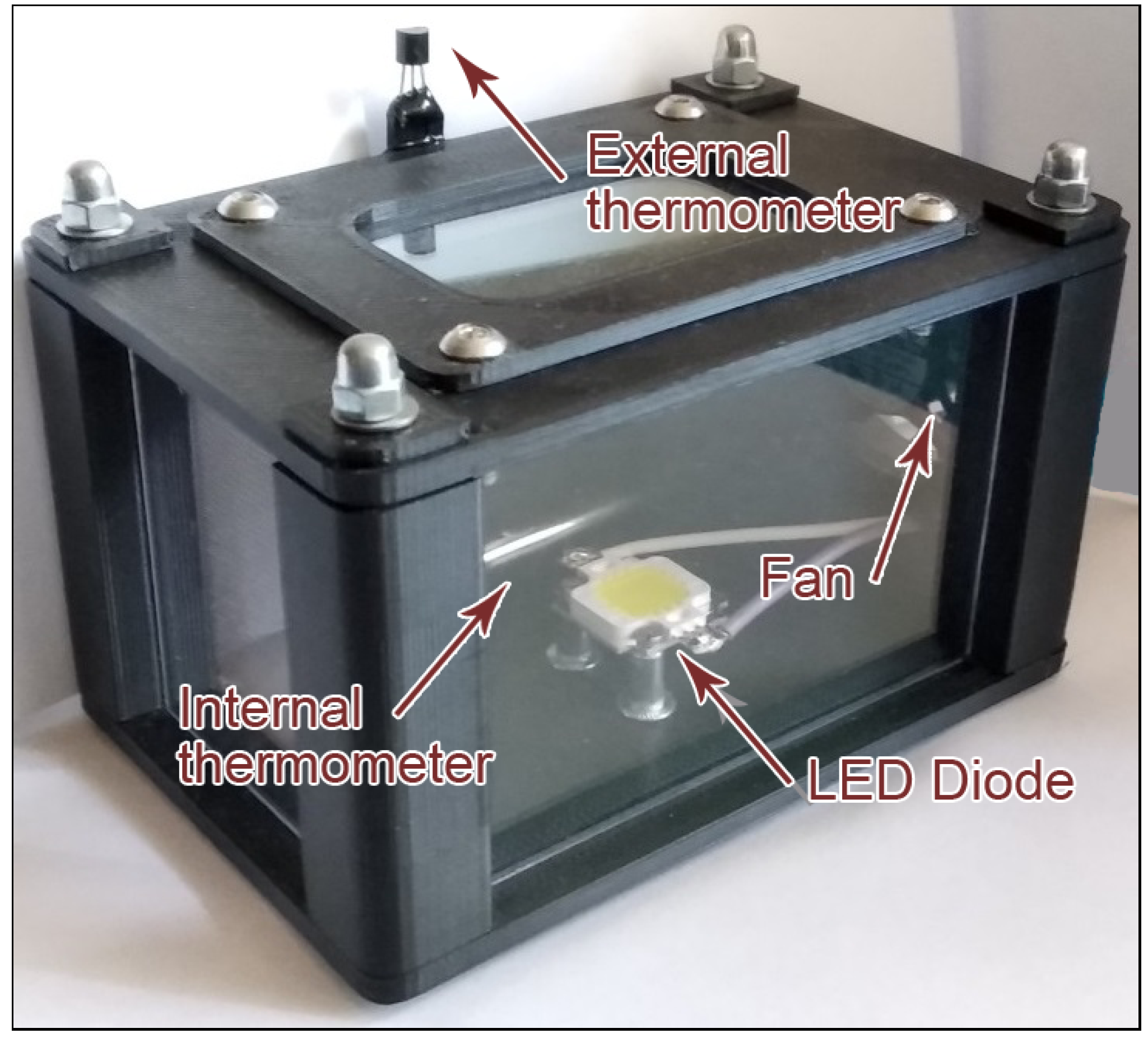
The case (
Figure 2) was designed in the Autodesk Inventor and was printed using ABS material. The general idea was to build a chamber that would be partially independent of the external environment and relatively small. As air volume has a great impact on the heating and cooling time of the air inside the chamber; only a small amount of free space was left for additional new measurement instruments. Besides the aspects of functionality, we decided to consider a visual aspect and used plexiglass windows, which enabled us to look inside the case. The dimensions of the box are shown in
Figure 3. The total outer case size is 120 × 80 × 70 mm.
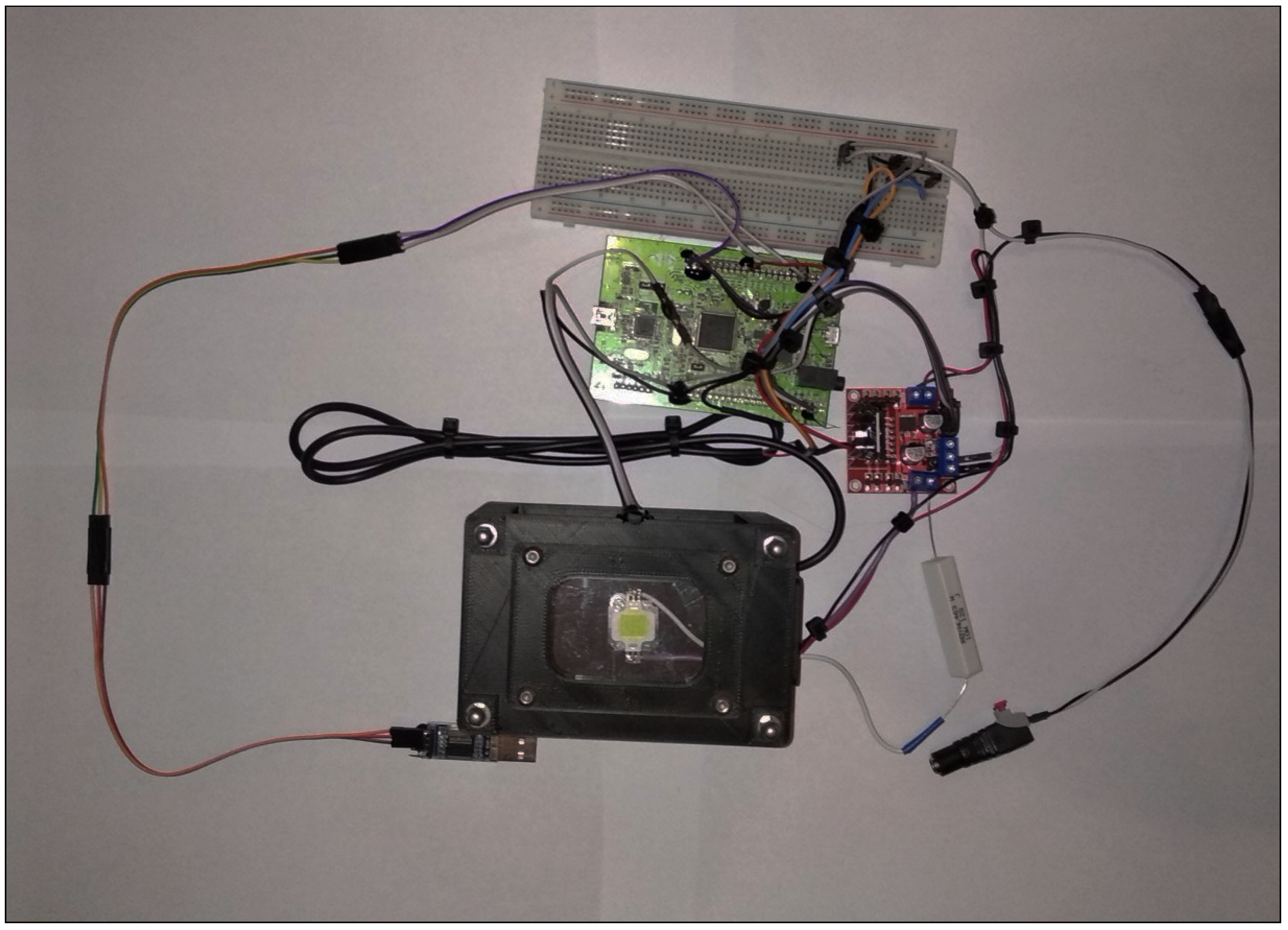
For measurement and control purposes, we decided to use the STM32F4 Discovery evaluation board, which is quite old and nowadays does not offer a great performance compared to other boards. We decided that if the solution works fine on this microcontroller, it can work even better on modern embedded platforms. Besides the board, we used two DS18B20 thermometers using a 1-wire interface, one L298N H-bridge controlled by PWM (pulse width modulation), one 40 × 40 × 10 12 V PC fan, one 10 W light-emitting diode (LED), and a PL2303HX converter, which allowed us to communicate with the board through the USART interface. One thermometer and one LED were put inside the chamber. The fan was placed on one side of the case. It allowed two goals to be reached: at low speed, it forced the airflow inside the case to equalize the temperature in the case, whereas at high speed, it cooled down the chamber. The microcontroller, H-bridge, and second thermometer were placed outside the case. We decided to use the led diode as a heater because it produces a large amount of heat and does not need a powerful power supply, which was confirmed in our internal tests in the past. The output power of the diode can be programmed to work between
and
. The power of the diode was reduced by a resistor, as suggested by the manufacturer. The fan can also be controlled, but in the range of
to
percent. The whole system is shown in
Figure 4. The peripherals, which are an integral part of the case, are shown in the
Figure 2.
An algorithm written in the C programming language controls the system. We used the STM32CubeIDE environment for board programming and Hercules software for communication over the USART interface. The code was divided into several parts that work together. The PF algorithm was rewritten from our original code in C# language [
18] and modified to work with the object.
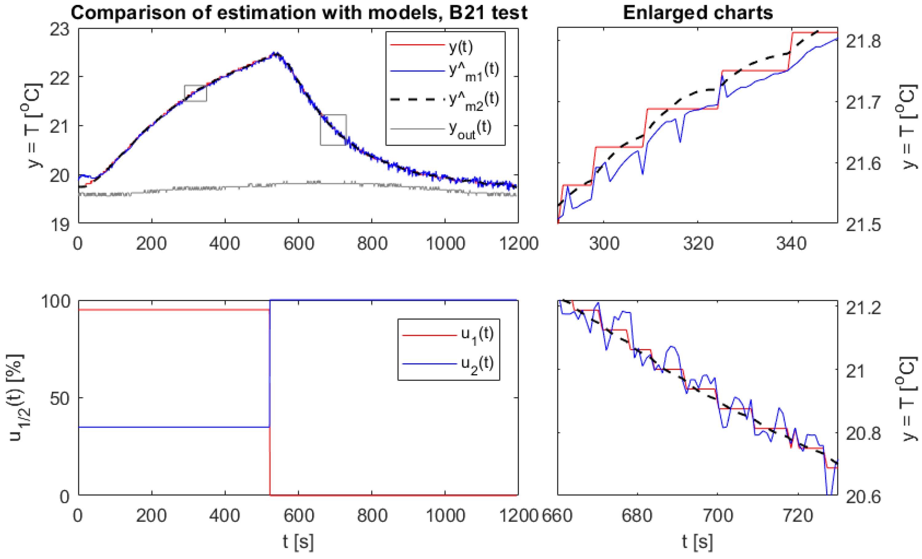
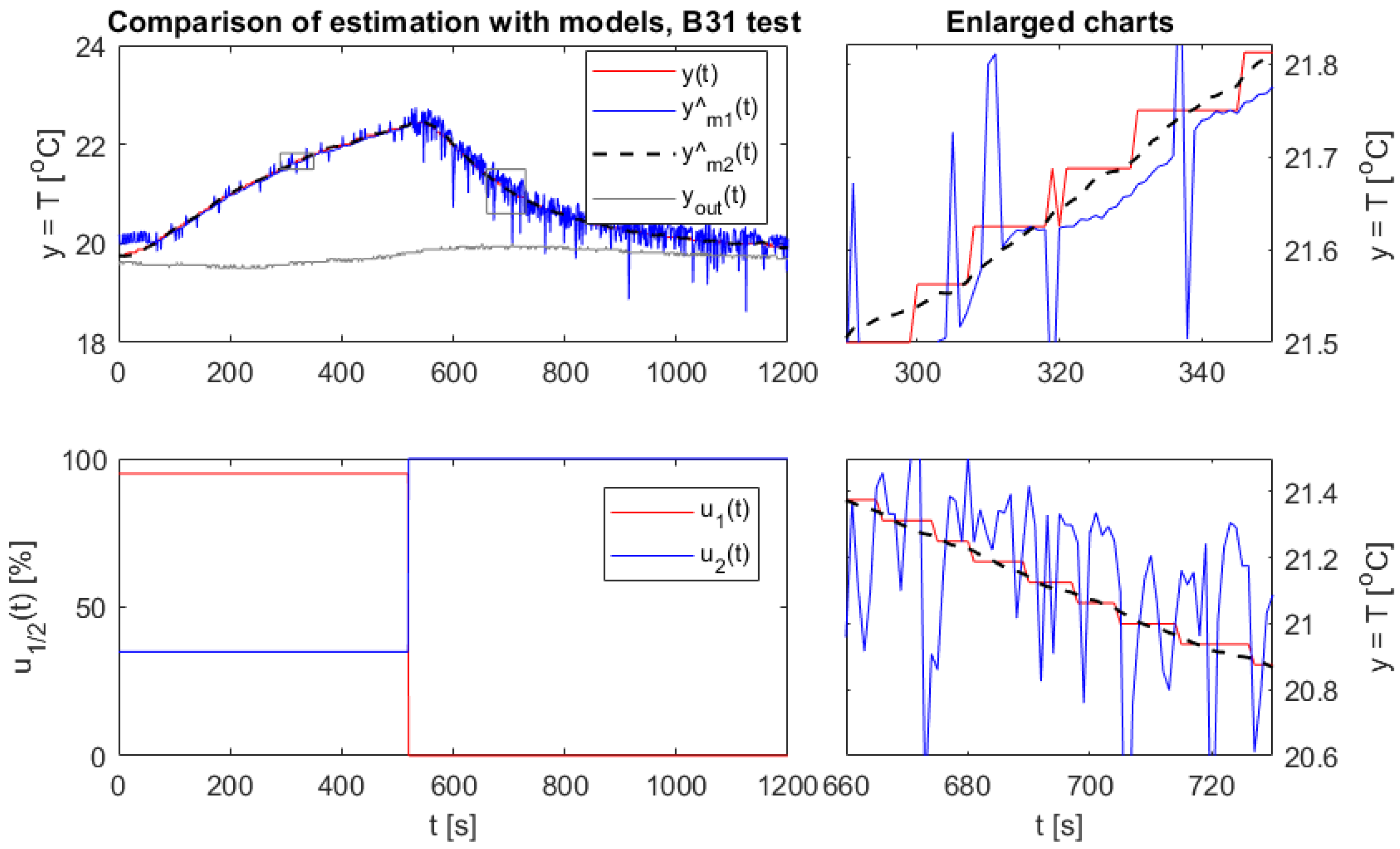
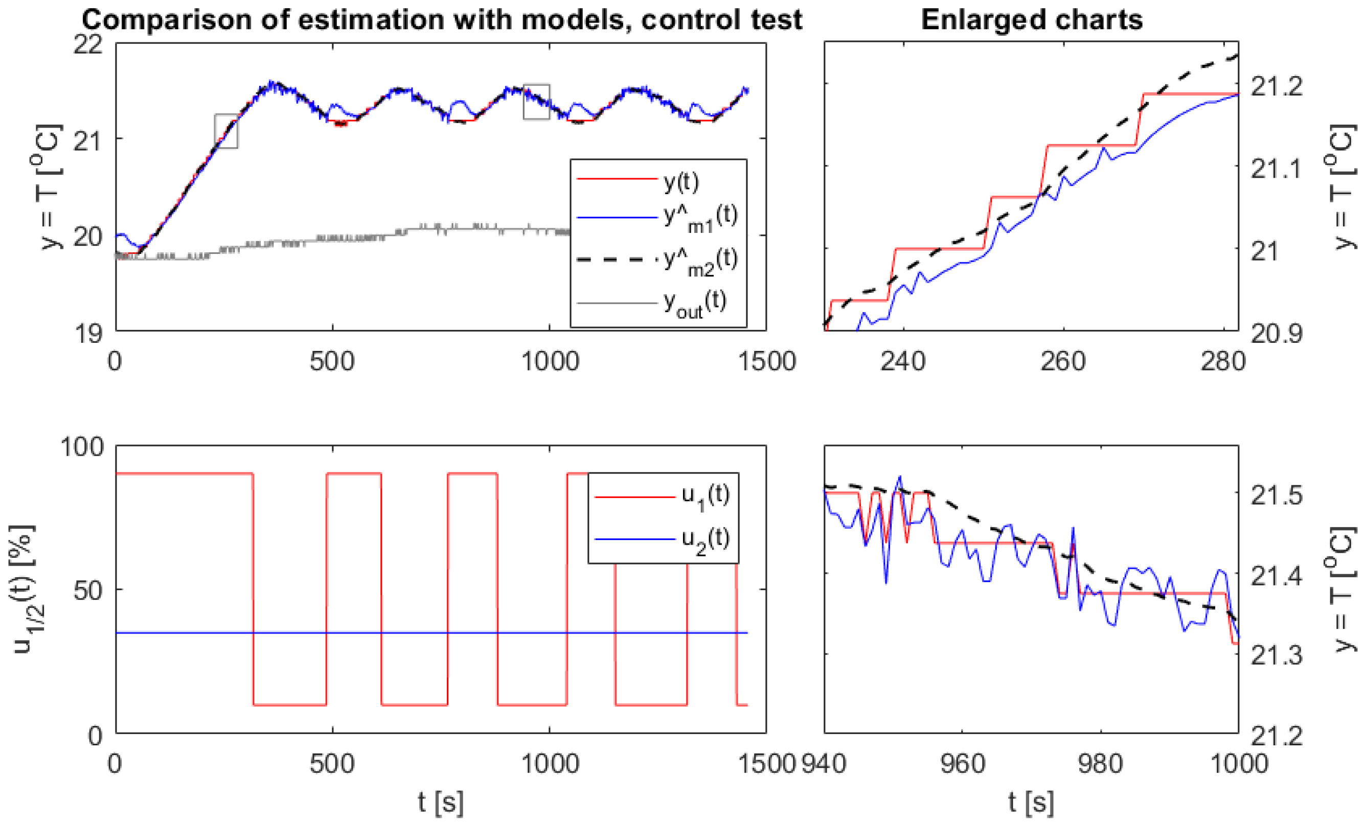
For the purpose of the estimation algorithm, the system was modelled by several mathematical models explained in the next section. The experiment can be in one of three states: heating, normal (keeping), and cooling down, according to the control inputs. Different models are used when the temperature decreases or when it increases. The switch of the models is based on the indoor temperature, the user-expected temperature, and the tolerance range: (the value results from the highest resolution of DS18B20, which is ). The measured temperature has an accuracy of . The second thermometer was not used directly in the system during the main tests, it was only used to perform comparison measurements.
4. Research Objects—The Mathematical Models
4.1. Simulation Object
The microcontroller was used in simulated tests and under real-world conditions. For simulation purposes, we used common particle filters examination [
4]. According to [
31], this object was first proposed in 1978 by Netto, Gimeno, and Mendes. The object is one-dimensional and has no external inputs; it is autonomous. The state change is only due to the presence of process noise. It is given by the discrete-time state-space equations
Simulation parameters: , , .
4.2. Real Object—Heating and Cooling System
To implement the particle filter algorithm for the real system, it was necessary to define a mathematical model of the tested object. In the literature, many examples involve the modeling and testing of the heating system [
32,
33,
34], but in this study, two-inertial objects were established. The detailed course of the thermal process identification experiment in different versions can be found in [
23]. The selected type of system is universal and is often used in the synthesis of a controller [
35]; it is given by a transfer function,
and the differential equation
where
t denotes continuous time,
K is the gain of the object, and
and
are the time constants. The notation
and
stand for
and
, respectively. Noises that affect the object have been ignored in the continuous-time model.
To identify the parameters of the object, tests with various amplitude step controls were carried out, during which the gain and time constant for the experiments were adjusted. Separate tests were carried out for the heating and cooling processes as different dynamic properties were then demonstrated by the models. Constant parameters were selected for the heating process (denoted by subscript h), while in the case of cooling (subscript c), the gain depends on the initial temperature that at the beginning of the experiment should be ideally equal to the temperature measured outside. The resulting parameters in the two modes are as follows:
heating: , , ;
cooling: , , .
Only two modes are assumed, namely, heating or cooling, in which the controls
(diode power—for heating) and
(fan power—for cooling) work, respectively. The built model can be considered as a jump system [
36,
37].
Continuous state-space equations, including phase variables, are given by
The system (
9) is then discretized with sample time
second using the Euler extrapolation method, and the obtained discrete state-space equations (dependent on the model parameters), including the modeling errors (
1), are shown below
It is worth noting that particle filters are applied in the heating process as well—an example such a process can be found in [
22]. In this paper, the complexity of the object has been limited to two state variables and one control signal due to implementation on a computationally weaker device. The noise of the process included in the PF (
1) compensates for the nonlinearity omitted in the model. To simplify the above considerations, the process noise in the transition function and the related disturbance transfer function were omitted. The PF algorithm takes into account the initial condition, namely, the temperature
, read in the first step of each experiment. Tests were performed for various noise variances.
4.3. Real Object—Estimation Using the Outdoor Temperature
A system given by the transfer function (
7) can be extended by using not just the measured temperature as an output but the difference between internal and external temperatures
. The parameters of this object were matched to the dynamics of changes in the new defined signal
y.
As it turns out in the test example, such a model will be very sensitive to disturbances in the form of, for example, changes in the outside temperature. Ultimately, when only was used in the transition model and when the initial value only depended on the outside temperature, the model performed better.
4.4. Real Object—Estimation without Using a Physical Model
In this model, the state-space equations are based not only on the dynamics of the system model under consideration but on the speed of temperature changes in the previous step. This approach allows for effective state estimation without knowing the exact dynamics of the process.
The discrete-time state variable
is the estimated temperature and accounts for the rate of change in the output of the previous step, as shown below:
The variable is used to store the history, representing the state variable from the previous step. Therefore, noise with zero error variance is added to it to obtain .
The matrix expression of the state-space equations, taking into account the process noises and based on (
11), is given by
It should be noted that the proposed system is autonomous. The change of state is caused only by the presence of system noise, and the parameters to be adjusted are the variances of the noises. The best estimation (based on the graphs) was observed for the parameters , , and .
This approach can be associated with dynamic linearization, which is used, among others, in the ADRC control algorithm [
38]. The result of this linearization is a model in the form of a double integrator. Therefore, the discrete-time characteristic polynomial for (
12) is
.
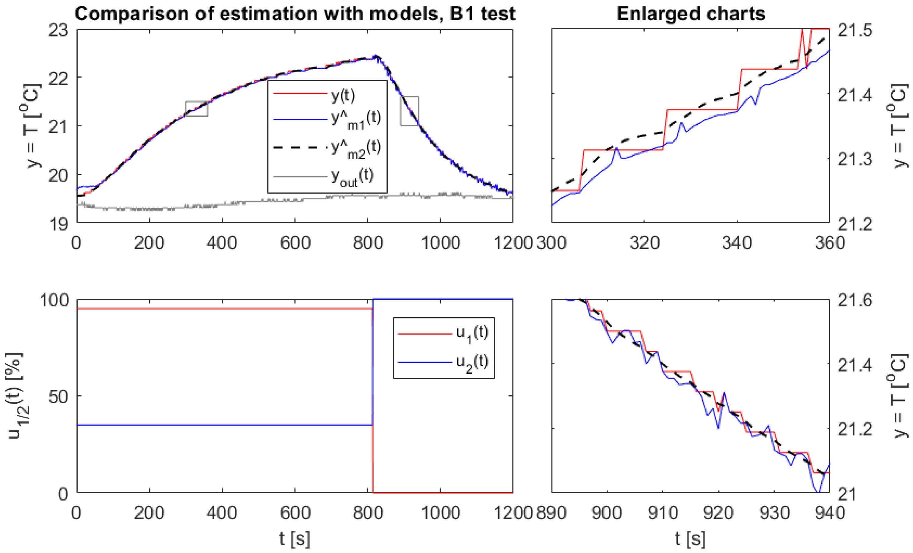
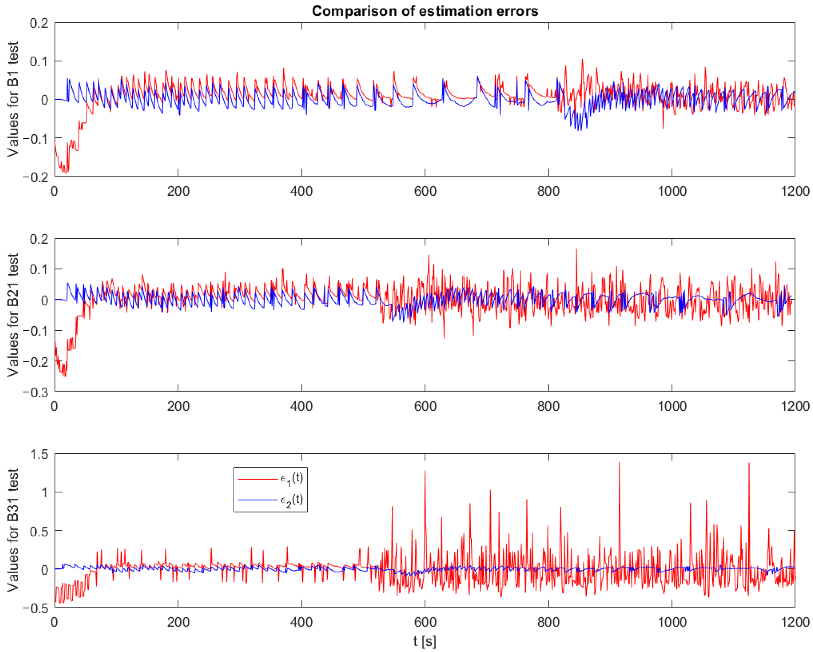
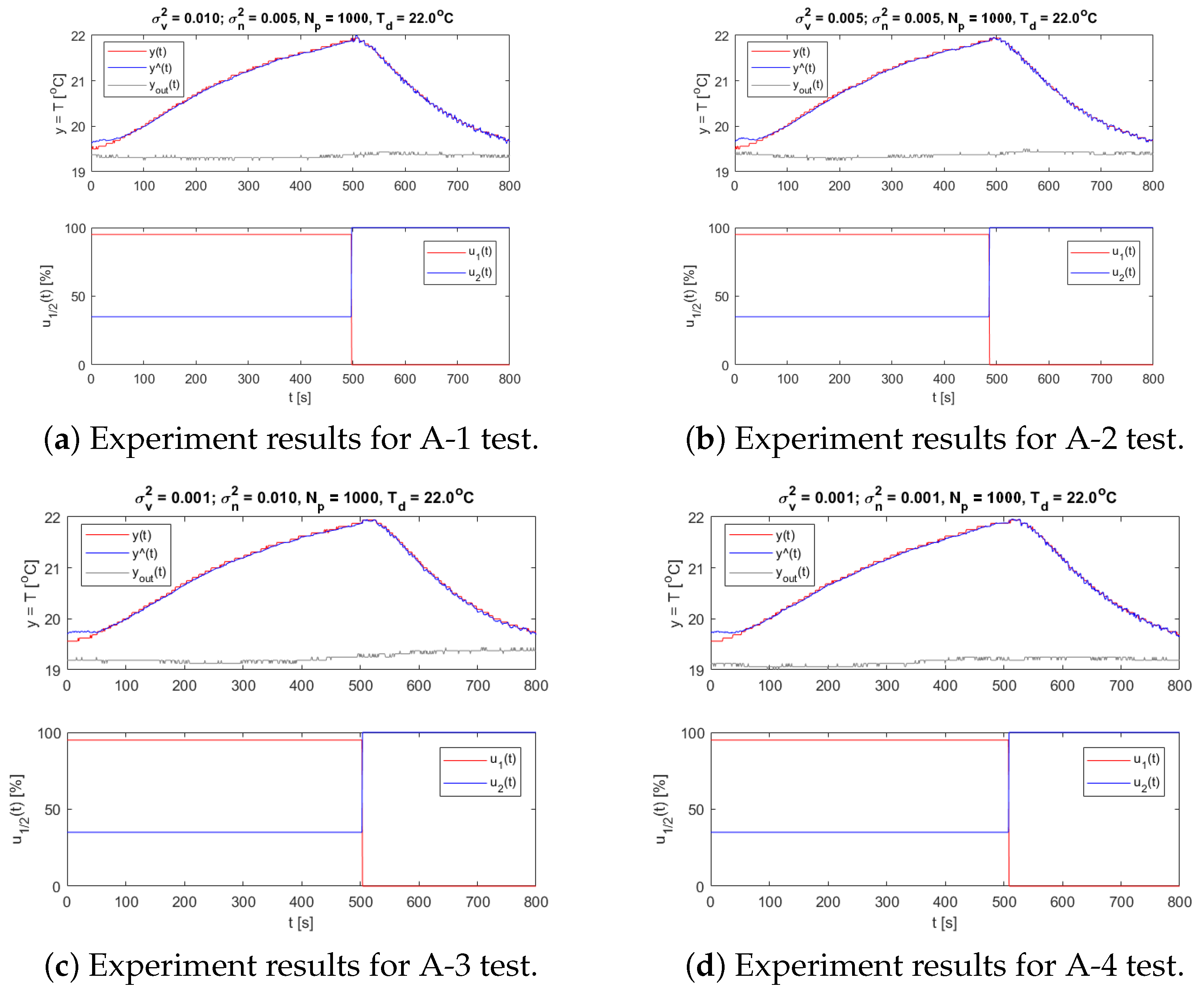
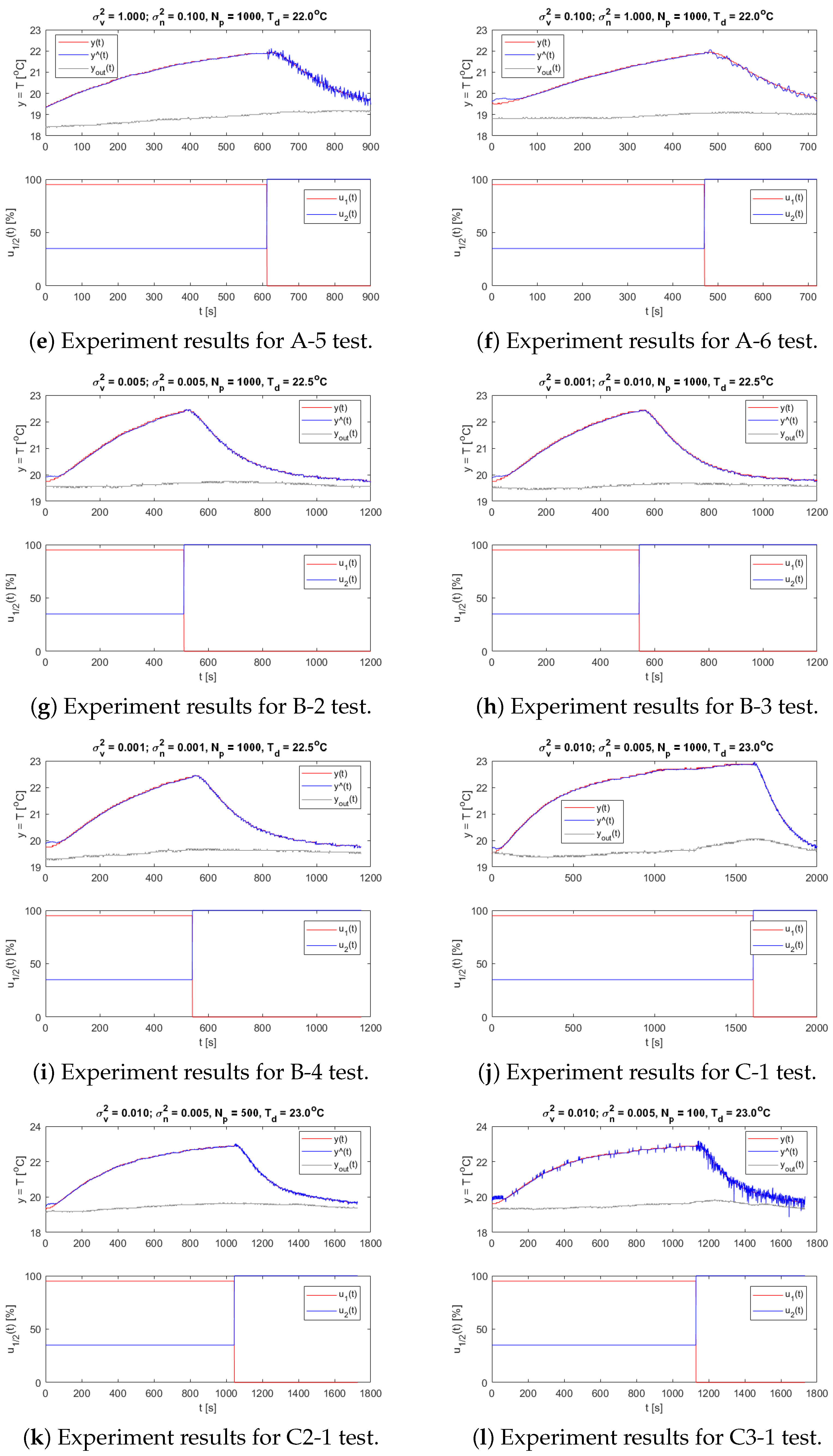
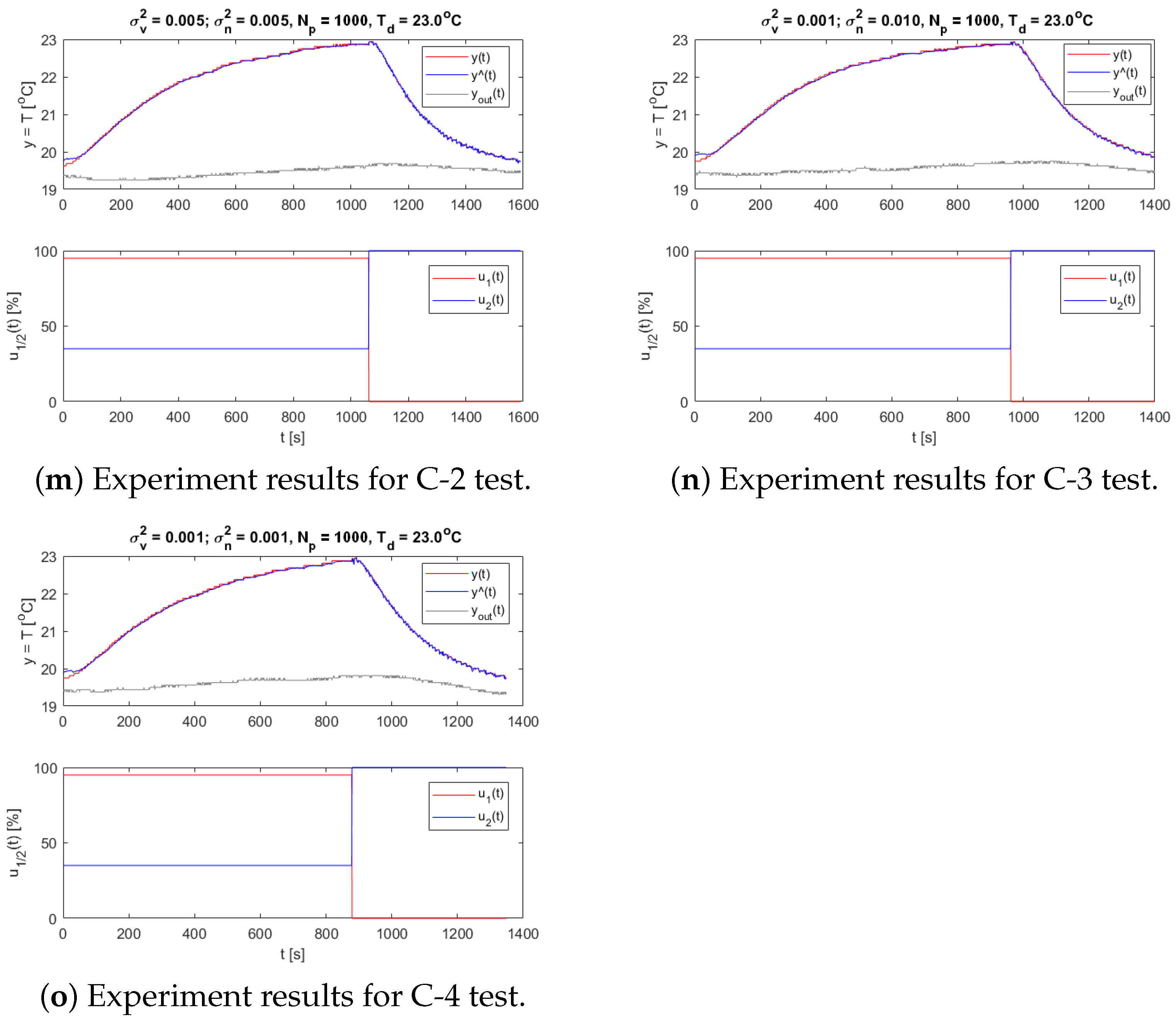
6. Discussion
Due to the simplicity of the assumed models, some features have been ignored, such as the nonlinearities of the system, the presence of two input signals at the same time, or the impact of the external temperature. This allowed for an effective implementation of an algorithm that operates with a real object on a device with low computing power. The mentioned features were effectively compensated for by the process noise generated in the particle sampling step. The heating process appeared to be more predictable, and the selection of parameters was unproblematic. The cooling process is also more complex to model.
The results were also obtained for various variances and temperatures (see
Appendix A). They show that the assumed values of the process and measurement noise variance have a critical impact on the quality of the PF performance. If the value of
is too high, the results affect the significant deviations of the mathematical model from the real object—in the particle sampling process, significant variance noise is added and later particles may not be able to match the actual measurements. For this research, better results were obtained in the case with lower variance values of the process noise (see
Figure A1d,e, for example), which proves that the model is well fitted, despite its simplification. It is also shown by the correct operation of the algorithm and the good adjustment of the estimate to the measurements in the case of different temperature values (operating points), as one can see in
Figure A1a,j.
The variance of the measurement noise is responsible for the inaccuracies of the sensor. In each test case, the best effects were observed for the value set comparable to the resolution of the measuring device. An overly high value of the setting resulted in the limiting of the confidence in the measurement in favor of the mathematical model. Ultimately, a compromise must always be made between trusting the model and the measurements. This allows us to compensate for any inaccuracies by the particle filter.
With correctly selected PF settings, a sufficiently large number of particles is needed for an effective state estimation. The number of particles must also be well suited to the computing power of the microcontroller to its capabilities.
In the case of precise process control, the use of feedback from the estimated value may improve the algorithm’s performance. Estimated values are commonly used in control, for example, in the active disturbance rejection control (ADRC) method [
39]. Improving the sensory information may be necessary, for example, if the resolution of the measuring device is too low.
7. Conclusions
In the article, an analysis of the possibilities of using the particle filter algorithm in an embedded system was carried out on real-time tasks. For the experiments, a special platform was built. It provided opportunities to perform tests on a real physical object. The main goal was to determine whether a relatively old platform, such as the STM32F4 Discovery board, is capable of performing calculations using particle filters, known for their high hardware requirements. Research has shown that it is possible, even in real-time scenarios. Our current research is focused on the real-time scenario with a much shorter sampling time, especially in tasks associated with drones. It is planned to also extend the research to uncontrolled environmental conditions. In the future, it is planned to carry out tests under various environmental conditions, for example, at very low or very high outdoor temperatures, e.g., by placing the box in an oven or fridge. We also plan to improve the quality of the measurements performed by the UAV on-board sensors. The work presented in this article is preparation for this.


