Abstract
Natural time analysis enables the introduction of an order parameter for seismicity, which is just the variance of natural time , . During the last years, there has been significant progress in the natural time analysis of seismicity. Milestones in this progress are the identification of clearly distiguishable minima of the fluctuations of the order parameter of seismicity both in the regional and global scale, the emergence of an interrelation between the time correlations of the earthquake (EQ) magnitude time series and these minima, and the introduction by Turcotte, Rundle and coworkers of EQ nowcasting. Here, we apply all these recent advances in the global seismicity by employing the Global Centroid Moment Tensor (GCMT) catalog. We show that the combination of the above three milestones may provide useful precursory information for the time of occurrence and epicenter location of strong EQs with in GCMT. This can be achieved with high statistical significance (p-values of the order of ), while the epicentral areas lie within a region covering only 4% of that investigated.
1. Introduction
Natural time has been introduced in 2001 [1,2,3] as a general method for the analysis of time series resulting from complex systems. It has been shown [4] that novel dynamical features hidden behind the conventional time series can emerge upon analyzing them in natural time. It has also been shown that such an analysis may reveal the dynamic evolution of a complex system and may identify when it enters a critical stage. As such, natural time analysis (NTA) is able to play a key role in predicting impending catastrophic events like the occurrence of earthquakes (EQs) [5,6,7,8,9,10,11,12,13,14] or cardiac arrest [15,16]. The applications of NTA that have appeared up to 2010 have been reviewed in the monograph by Varotsos et al. [4], providing examples in various disciplines such as Statistical Physics, Condended Matter Physics, Geophysics, Seismology, Biology, and Cardiology. Since 2011, various newer applications have appeared in a variety of scientific fields, such as condensed matter and materials [17,18,19], geosciences [20,21,22,23,24,25,26,27,28], engineering [29,30,31,32,33,34,35,36], climate change [37,38,39,40], and cosmic rays [41]. Earthquake nowcasting introduced by Rundle et al. [42], which is the most recent method for seismic risk estimation by means of the earthquake potential score (EPS), is also based on the concept of natural time. Earthquake nowcasting has found wide successful applications in estimating the seismic risk in global megacities [43], in the study of induced seismicity [44], in the study of temporal clustering of global EQs [45], in clarifying the role of small EQ bursts in the dynamics associated with large EQs [46], in understanding the complex dynamics of EQ faults [47], in identifying the current state of the EQ cycle [48,49], and very recently in volcanic eruptions [50].
We focus, hereafter, on the applications of NTA in seismicity. It has been shown that the variance of natural time may be considered as an order parameter for seismicity [5,51,52,53,54,55] as well as for acoustic emission before fracture [19,22] or for other self-organized critical phenomena such as ricepiles [56] and avalanches in the Olami–Feder–Christensen [57] earthquake model [58] or in the Burridge–Knopoff [59] train model [60]. In such cases, the new phase is the strong EQ (or large avalanche), which leads to a value of very close to zero, see, e.g., Varotsos et al. [4,5]. It has been also observed that exhibits significant fluctuations before or after strong mainshocks [61,62], which are reflected in its statistical distribution [63,64].
For the quantification of these fluctuations, the variability , defined in [61] as the ratio of the standard deviation over the mean value of , in an EQ catalog excerpt (i.e., a part of an EQ catalog consisting of W consecutive EQs) has been employed. It was found that when the size W of the EQ catalog excerpt is comparable with the number of EQs that usually occurs during the lead time of Seismic Electric Signals (SES) activities minimizes before the strongest EQs in California and Greece [65]. We note that SES are low-frequency variations of the electric field of the Earth that precede EQs, see, e.g., References [4,66,67,68,69,70,71,72,73,74,75]. Moreover, characteristic (local) minima of have been identified in California [76], Japan [11], Mexico [77,78,79], Eastern Mediterranean [80,81], and Global seismicity [13,82] before the strongest EQs, i.e., those in the EQ catalog having a magnitude M greater than or equal to a target threshold , , and these minima are statistically significant precursors [83,84]. Interestingly, the appearance of these minima has been related [85] to the emission of SES activities and are also simultaneous with changes in the long-range correlations of the EQ magnitude time series [64,86,87] (cf. an extensive related review has been published by Varotsos et al. [88]). Finally, almost a year ago, the combination of the study of the fluctuations of the order parameter of seismicity provided an earthquake nowcasting method of estimating the epicenter of a forthcoming strong EQ, which was based on the self-consistent construction of average EPS maps [79,81].
The present paper focuses on the study of the most recent global seismicity (see Figure 1) by means of NTA when incorporating the advances of the average EPS maps as well as taking advantage of the development of long-range correlations in the EQ magnitude time series upon the appearance of minima. We will see that the combination of these methods allows —within a nine-month time window and inside a region covering only 4% of the total studied area—an estimation of the time and place of occurrence of all EQs with only two false alarms during the period from 1 January 1976 to 31 January 2022. The paper is organized as follows: In the next Section 2, the EQ data and the methods that will be used are briefly explained and the results are presented in Section 3. Their discussion follows in Section 4, while our Conclusions are presented in Section 5.
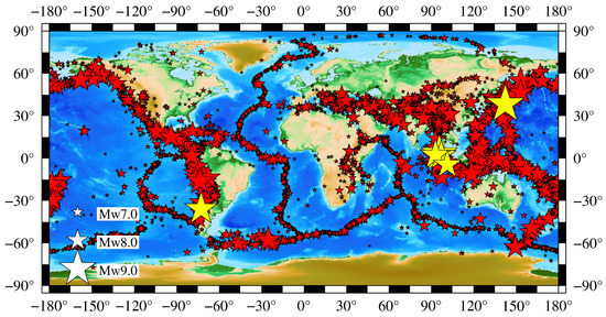
Figure 1.
The map shows global seismicity with all EQs of as reported by GCMT during the period from 1 January 1976 to 31 January 2022 (see References [89,90] and Section 2.1). The EQs with appear with yellow color, while for with red color. ETOPO1 Global Relief Model [91] was used to integrate the land topography and ocean bathymetry. This map was made using Generic Mapping Tools [92].
2. Materials and Methods
2.1. EQ Data
We used the available data from the Global Centroid Moment Tensor project [89,90] (GCMT). Currently, the data covers the global seismicity since the 1st of January of 1976 until 31st of January 2022. For the period January 1976 to end of December 2020, we used the 1976–2020 CMT catalog from https://www.ldeo.columbia.edu/~gcmt/projects/CMT/catalog/jan76_dec20.ndk (accessed on 23 May 2022) address while for the period since the 1st January 2021 to end of January 2022 we used the monthly CMT catalogs from https://www.ldeo.columbia.edu/~gcmt/projects/CMT/catalog/NEW_MONTHLY/ (accessed on 23 May 2022) (The home page for all catalogs is the http://www.globalcmt.org/CMTfiles.html (accessed on 23 May 2022)). Following Reference [13], we considered only the EQs with (moment) magnitude (or simply M) greater or equal than 5.0, i.e., , whose epicenters are shown in Figure 1. A frequency-magnitude diagram, see, e.g., Figure 2, provides a means for assessing the approximate level of completeness of the catalog. The data for the whole period examined 1976–2022 suggests linearity of the slope of the frequency-magnitude relation down to a magnitude of 5.0 (Figure 2a), which is the same for the later period 2001–2022 (Figure 2c), while for the earlier period (1976–2000, Figure 2b), the data are more consistent with a break in the slope near . These results are compatible with those of Ekstrom et al. [90], who, when using the same catalog, found a completeness magnitude threshold of 5.0 for the period 2004–2010, while for the earlier period, they reported a break in the slope near 5.3 or 5.4, see their Figure 5.
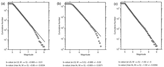
Figure 2.
Frequency–magnitude diagram for earthquakes in the GCMT catalog. Estimated b-values with least squares (labeled ‘w LS’) and the maximum likelihood (labeled ‘max lik’) method are also shown at the bottom of each panel. (a) For the whole study period (1976–2022), (b) for the period 1976–2000, and (c) for the period 2001–2022, using the ZMAP software [93]. The number of earthquakes is counted in bins of 0.1-magnitude-unit width.
2.2. Natural Time Analysis Background and Order Parameter Fluctuations for Seismicity
When a time series comprises N EQs, we define natural time for the occurrence of the k-th EQ as . Considering that the quantity is proportional to the energy emitted during the l-th EQ, is the normalized energy of the k-th EQ and is estimated from the seismic catalog. Here, we used as the scalar seismic moment M reported in GCMT, i.e., (M (see References [1,4,13]). Alternatively, the quantity can be calculated directly from the moment magnitude [94] or by converting the magnitude reported in the catalog to , see, e.g., Reference [95]. As already mentioned, the variance of natural time serves as an order parameter [4,5,19,56] for seismicity:
In order to calculate the fluctuation of within an excerpt of the EQ catalog comprising W consecutive EQs, we have to calculate a variety of values corresponding to this excerpt. Let us assume that the first EQ of the excerpt corresponds to energy . We can then form sub-excerpts of consecutive N = 6 EQs of energy and natural time each (cf. at least six EQs are needed [5] for obtaining reliable ). By substituting in Equation (1), we can calculate and by sliding over the excerpt of W EQs setting a totality of values of are estimated. We repeat this calculation for , thus, obtaining an ensemble of values of . Then, we compute the average and the standard deviation of the thus obtained ensemble of values. The fluctuation of is quantified by the variability defined to be:
in order to follow the time evolution of , this value is assigned to the -th EQ in the EQ catalog. As stated in the Introduction, the number W is chosen [65] to correspond to the number of EQs that, on average, occur during the average lead time of an SES activity that ranges from a few weeks to months (see Chapter 7 of Ref. [4]), i.e., a period of a few months.
2.3. Detrended Fluctuation Analysis of EQ Magnitude Time Series
The Detendred Fluctuation Analysis (DFA) was first introduced by Peng et al. [96] in a biology context. They presented it as an alternative method which allows detecting and quantifying long-range correlations in non-stationary time series, and which also is independent of the established input [96]. In general, the DFA presents some assets over other traditional methods. For instance, it detects intrinsic self-similarity in many nonstationary time series, especially in those that have a slow trend variation; also it prevents from illusory self-similarity. In the past few years, the DFA method has been used to effectively analyze a variety of time series involving several fields of knowledge, such as DNA [96,97,98], cardiac dynamics [99,100,101], neuronal oscillations [102], heartbeat fluctuation [103,104], meteorology [105], etc.
The method consists of the following: beginning with a time series or signal , with and N the length of the time series, the steps of the DFA method are:
1. The signal profile is created. We do this by integrating with respect to its mean, i.e., by calculating the cumulative sum of the time series:
where is the mean:
2. The integrated time series, i.e., the profile is divided into equal epochs or boxes of length n. Then, for all boxes, a least squares line is fit to the data in the corresponding box, which represents a local trend in that box. From the linear fit, we use the y-coordinate to define the local trends, .
3. We detrend the profile , by substracting the local trend, , in each one of the boxes, i.e., we obtain:
4. The root mean square (rms) of the integrated and detendred time series is computed:
5. We repeat steps 2, 3, and 4 for each one of the characteristic time scales (box sizes) set in the time series.
6. Finally, we compute the linear fit between and the box size n: . The slope of a linear fit between log-rms () and log-scales () provides the scaling (or DFA) exponent .
If , the signal or time series is anti-correlated; if , the signal is uncorrelated (white noise); if , the signal is correlated; and if , the signal is -noise (pink noise). In the present paper, we employed the DFA [96,106] computer code dfa.c developed by J. Mietus, C.-K. Peng, and G. Moody available from Physionet [107] at https://www.physionet.org/content/dfa/1.0.0/dfa.c (accessed on 1 September 2018).
2.4. Earthquake Nowcasting and EQ Potential Score
Rundle et al. [42] introduced earthquake nowcasting for estimating the seismic risk through the current state of fault systems in the progress of the EQ cycle (for the latter, see References [46,48,49]). Earthquake nowcasting employs [42] natural time and uses an EQ catalog to calculate from the number n of ‘small’ EQs, defined as those with magnitude but above a threshold , i.e., , that occurred after the last ‘large’ EQ, the level of hazard for such a large EQ. Thus, the number n stands for the waiting natural time or interoccurrence natural time. The EQ catalogs used [42,43,79,81,108,109,110,111,112] for earthquake nowcasting are publicly available global EQ catalogs. Here, we used the GCMT EQ catalog, see Section 2.1. The magnitude threshold has been considered in accordance with Reference [13], while in view of the fact that natural time analysis, by means of the method presented in Reference [51], has revealed that EQs with are correlated globally [52,113]. The current number of the ‘small’ EQs since the last occurrence of a ‘large’ one is compared to the cumulative distribution function (CDF) of the interoccurrence natural time . To estimate , it should be ensured [42] that we have enough data to span at least 20 or more ‘large’ EQ cycles. The EQ potential score (EPS) equals the CDF value,
and measures the level of the current hazard, see Figure 3a.
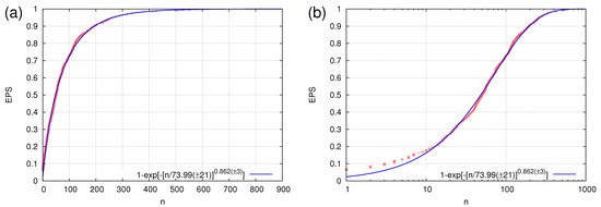
Figure 3.
The EPS versus the number n of ‘small’ EQs with that occur during the period between two ‘large’ EQs of magnitude in the globe (see Figure 1) as estimated by the empirical cumulutive distribution function (red plus symbols) or its Weibull model fit [109,110,112] (blue line). Panels (a,b) correspond to lin-lin and lin-log diagrams, respectively. They have been both drawn for the readers’ better information.
The seismic risk for various cities of the world was estimated [42,43,108,109,110,112] by first calculating the CDF within a large area and comparing it with the number of the ‘small’ EQs around the city, i.e., those that occurred within a circular region of epicentral distances , since the occurrence of the last ‘large’ EQ in this region. Rundle et al. [43] proposed that the seismic risk for the city can be found by substituting with in Equation (7), i.e., EPS , because EQs exhibit ergodicity [114,115,116].
In the present study, we focus on the period from 1 January 1976 to 31 January 2022 and make use of the GCMT catalog with and . This leads to the empirical CDF shown in Figure 3, which includes 614 EQ cycles. In this figure, we observe that the fit
using the Weibull distribution provides a fair approximation with root mean square of residuals [117] equal to 0.017. This is in accordance with the results found in References [79,81,110].
2.5. Average EPS Maps
A self-consistent method of producing average EPS maps, also written ⟨EPS⟩ maps, using a radius R has been suggested and applied to the Eastern Mediterranean area in Reference [81] and further developed by Perez-Oregon et al. [79]. To construct such a map, one first estimates EPS for disks of radius R at the points of a lattice to obtain EPS and then averages for each point the estimated EPS values within the same radius R, i.e.,
where the summation is restricted to the lattice points whose distance from the observation point is smaller than or equal to R, and N stands for the number of lattice points included in the sum.
It has been shown (see Figure 6 of Reference [79]) that the study of ⟨EPS⟩ close to the epicenters of forthcoming strong EQs exhibits a logarithmic dependence on R, reminiscent of the Green’s function of the Poisson equation in two dimensions, while the mean value of ⟨EPS⟩ over all the lattice points scales with R as a power law with an exponent , i.e, , see Section 3 and Equation (12) of Reference [81]. A clear relation between such made ⟨EPS⟩ maps and the epicenter of an impending strong EQ has been observed in the respective regional studies [79,81]. Here, we first estimated EPS for disks of radius R centered at each point of a square lattice covering the globe, and then averaged these EPS values within the same radius R.
2.6. Receiver Operating Characteristics
For the estimation of the statistical significance of an EQ prediction method, we use the Receiver Operating Characteristics (ROC) method [118], which is a plot of the hit rate (or True positive rate) against the false alarm rate (or False positive rate). ROC, therefore, depicts the quality of binary predictions.
In particular, the ratio of the cases for which the alarm is ON and a significant event occurred over the total number of significant events defines the hit or true positive rate. The false alarm rate, on the other hand, is defined as the ratio of the cases for which the alarm was again ON but no significant event occurred over the number of non-significant events. A predictor will be useful only if the hit rate exceeds the false alarm rate. In addition, if a prediction is random, it will generate an equal number of hit and false alarm rates on average, and the corresponding ROC curves will have fluctuations depending on the number P of significant events (positive cases) and the number Q of non-significant events (negative cases) to be predicted.
The area A under the curve (AUC) in the ROC plane is what determines the statistical significance of an ROC curve [119]. As it was shown in Reference [119], , where U follows the Mann–Whitney U-statistics [120]. In 2014, the statistical significance of ROC curves was visualized [121] using the envelopes of confidence ellipses, called k-ellipses, which cover the entire ROC plane. Using A, one can measure the probability p to obtain an ROC curve passing through each point by chance.
3. Results
Following Reference [13], we calculated for and (see Figure 4) in order to identify the precursory—within 9 months (for example compare the second with the fourth column of Table 1)—fluctuation minima that precede all EQs in global seismicity. A fluctuation minimum can be considered as ‘precursory’ when the following conditions [13] are satisfied: A local minimum of either or is considered as such if it is smaller than its 15 previous and 15 future values. Since we assume [11] that there exists a single critical process (one fluctuation minimum), 90% of the EQs that lead to the minimum should appear in the minimum . Moreover, since this process is characteristic, the ratio should lie within the limits defined by the minima preceding the EQs [13], i.e., or:
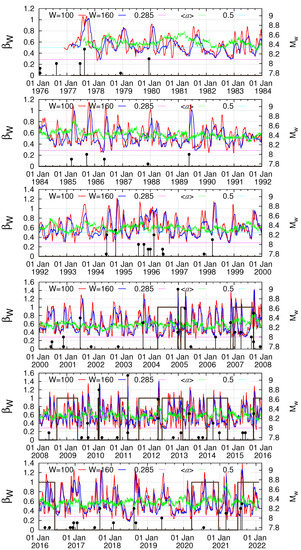
Figure 4.
The order parameter fluctuations for global seismicity as depicted by the variabilities for (red) and (blue) during the period from 1 January 1976 to 31 January 2022. The EQ magnitudes, which are read in the right scale, are denoted by the (black) vertical lines ending at solid circles. The horizontal magenta and cyan lines correspond to the values 0.285 (=) and 0.5, respectively. The thick dark brown line resembling a dichotomous (ON/OFF) signal, indicates when an alarm is ON by taking the value 1. Otherwise, there is no alarm. The average DFA exponent discussed in Section 4 is also shown by the green lines.

Table 1.
The ‘precursory’ fluctuation minima, i.e., the variability minima that satisfy Conditions (10) and (11), together with DFA exponents , , and their mean value . The exponents typed boldface lie outside the range defined by the corresponding exponents estimated for the precursory variablility minima that preceded all EQs with . For each row, a label is also inserted to express whether it is a hit (H1 to H6) or a false alarm (FA1 to FA6). For the hits, a brief reference to the predicted EQ is inserted in the corresponding column, for more details, see Table 2.
Finally, should be smaller than the shallowest precursory to EQ, denoted by , i.e.,
and , as found in Reference [13].
The analysis of and leads to the 12 ‘precursory’ fluctuation minima shown in Table 1. In this Table, we also insert the two DFA exponents and , which were calculated from the EQ magnitude time series on the date of when considering either the preceding 160 or 300 EQs, respectively. They lead to a better classification of the ‘precursory’ fluctuation minima as it will be discussed in the next Section. These ‘precursory’ fluctuation minima were followed within 9 months by the 13 strong EQs labeled by H1 to H6 and FA1 to FA6b in Table 2.
Table 2.
List of the 15 strong EQs discussed in the text. In each case, in addition to the EQ magnitude, epicenter location, and date, a label is also ascribed by relating the EQ to minima. These labels have the following meaning: H1 to H6 correspond to true positive precursory variability minima, FA1 to FA6 to false positive variability minima (FA6a and FA6b are related to the same minimum FA6 of Table 1), while cases C1 and C2 correspond to the minima of observed on 24 April 2017 and 6 July 2018, respectively. For the details of the precursory variability minima see Table 1. The EQ names for EQs with are typed boldface.
In accordance with References [79,81], we used the date of as the last date of the EQ catalog and constructed the ⟨EPS⟩ maps for km. The latter are shown in Figure 5 and Figure 6. In these two Figures, the epicenters of the strong EQs that took place (within 9 months) after the ‘precursory’ fluctuation minimum (see Table 1 and Table 2) are also inserted. In Figure 6g,h, the ⟨EPS⟩ maps were constructed on the dates 24 April 2017 and 6 July 2018, respectively, when non-‘precursory’, i.e., not satisfying Conditions (10) and (11), fluctuation minima were observed, see Figure 4, but were also followed by the two strong EQs labeled C1 and C2 in Table 2.
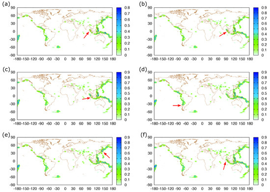
Figure 5.
Average EPS maps calculated on the date that minimizes (see Table 1) for the case of coarse grain radius km. Panels (a–f) correspond to the EQs Sumatra–Andaman, Sumatra–Nias, Sumatra–Indonesia, Chile, Tohoku–Japan, and Indian Ocean, respectively (see also Table 2). The epicenters of the latter EQs are depicted by red circles indicated by arrows for the readers’ convenience. The values of at the grid point closest to each epicenter location vary from 7% to 50%.
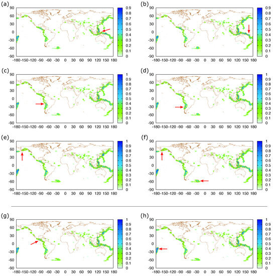
Figure 6.
Average EPS maps calculated on the date that minimizes (see Table 1 and Section 3) for the case of coarse grain radius km. Panels (a–h) correspond to the EQs Papua–Indonesia, Solomon Islands, Iquique–Chile, Illapel–Chile, Alaska, Chignik–Sandwich, Chiapas, and Fiji, respectively (see also Table 2). The EQ epicenters are depicted by red circles indicated by arrows for the readers’ convenience. The values of at the grid point closest to each epicenter location vary from 7% to 77%.
4. Discussion
NTA enables the detection of magnitude correlations [4,51] when comparing the distribution of the order parameter of seismicity of the original EQ catalog with that of randomly shuffled copies of the same catalog. This has led, as already mentioned, to the conclusion that EQs with are correlated in global scale [52,113]. This lies behind our selection of for earthquake nowcasting in Section 2.4. Indeed, the fact that EPS can be described by the Weibull distribution of Equation (8) with an exponent which is definitely different from unity (Poissonian statistics) provides an independent verification of the presence of these correlations.
We now turn to the statistical properties of average EPS maps. We first focus on the statistics of ⟨EPS⟩ at the lattice points closest to the epicenters of the six EQs with in GCMT, i.e., those depicted in Figure 5 and typed boldface in Table 2. Figure 7 depicts their average value together with their standard deviation versus the coarse grain radius R. We observe the presence of a logarithmic singularity in the fitting function of in a fashion similar to that identified in Reference [79]. This is reminiscent, as mentioned, of the two-dimensional Green’s function for Poisson equation and reflects the fact that the future EQ epicenters (cf. ⟨EPS⟩ maps were drawn on the date of their preceding , see Table 1) act as ‘sources’ in these maps. This strengthens the potential of earthquake nowcasting to be generalized to forecasting, see also Reference [111]. Let us now consider the R dependence of the mean value:
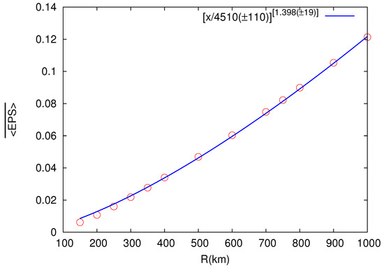
where the summation is made over all the lattice points , estimated numerically in an average EPS map drawn with a coarse grain radius R, while is a length scale. The average value of estimated for the ⟨EPS⟩ maps related to the six EQs with , i.e., those depicted in Figure 5, versus the coarse grain radius R, can be seen in Figure 8. In Section 3 of Reference [81], it has been shown that may take the form:
where is related to the fractal dimension [122] of EQ epicenters. Figure 8 reveals that for the global seismicity, which does not differ much from the value 1.32 , estimated by the same method in the Eastern Mediterranean area [81].
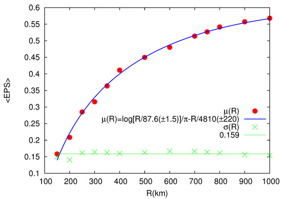
Figure 7.
The average value (red bullets) together with the standard deviation (green crosses) of the values closest to each epicenter of the six EQs (see Table 2 and Figure 5) versus the coarse grain radius R. The expressions for the fitting function (blue) and the average value of (green horizontal line) are also shown.
According to the regional studies of References [79,81], when drawing an ⟨EPS⟩ map on the date of a variability minimum of seismicity, we can have an estimation of the epicenter of a future strong EQ. An inspection of Figure 5 and Figure 6 reveals that this is also true for global seismicity. Especially for the six strongest EQs of during our 46 years study period, Figure 5 reveals that for 200 km ⟨EPS⟩ at the lattice points closest to their epicenters takes values from 7% to 50%. Only 4% of the lattice points examined lie in this range of EPS values, showing that ⟨EPS⟩ maps for 200 km certainly provide information about the epicenter of a future strong EQ. This is also strengthened by the fact that even when we consider the case of Figure 6, which inlvolves smaller in magnitude EQs (but also strong with ) the corresponding ⟨EPS⟩ closest to the epicenters vary from 7% to 77%, which correspond to just 5% of the points of the lattice on which we made the calculation. We have to mention that in Figure 6g,h, we also included the ⟨EPS⟩ maps estimated on the dates of , although such minima do not satisfy the Conditions (10) and (11) to be considered as ‘precursory’ fluctuation mimina. This was made in order to show that the methodology of Reference [79], where we just considered local variability minima for drawing ⟨EPS⟩ maps, can also be applied in the global scale. In summary, we can say that the combination of earthquake nowcasting with the study of the variability minima of the order parameter of seismicity not only reveals useful information for the epicenters of the EQs that followed the ‘precursory’ fluctuation minima identified in Reference [13], i.e., those inserted in the first nine rows in Table 2, but may also highlight the epicenters of the most recent five strongest EQs in the globe during the almost seven year period from 1 January 2015 to 31 January 2022.
As already mentioned, in Reference [13], the Conditions (10) and (11) have been established for identifying ‘precursory’ fluctuation minima in the global scale by means of NTA. Opening a prediction window of nine months on the date of appearance of , this initial study has led to six true positive results (hits) preceding the strongest EQs in the GCMT catalog. When such a strong EQ occurs, the alarm window terminates. The study of Reference [13] also produced three false alarms leading to the corresponding three nine-month windows, which do not include any EQ in the last but one panel of Figure 4. These false alarms are related to the order parameter fluctuation minima that preceded the Papua–Indonesia, Solomon Islands, and Iquique–Chile EQs; see the newly constructed ⟨EPS⟩ maps in Figure 6a–c, respectively. Apart from providing this epicentral information, the present work also extends that study for the period from 1 October 2014 to 31 January 2022. The present study led to the alarms shown by the brown binary (0/1)—or dichotomous (ON/OFF)—line in Figure 4. A careful inspection of this Figure reveals that three more false alarms appear, see the last three rows in Table 1. Interestingly, these three new false alarms could be correlated with the two strongest EQs of that took place since 1 October 2014, while the third would be related with the Alaska EQ [123] that took place on 22 July 2020, the stress changes of which triggered [124] the 2021 Chignik EQ [125]. Thus, one may support the view that these false alarms are at least related with the strongest EQs during the last seven years, none of which, howewer, had magnitude .
At this point, we need to incorporate the results of Varotsos et al. [86] that showed the interconnection of magnitude time series correlations with the minima of the fluctuations of the order parameter of seismicity and SES. Since References [13,86] were prepared almost simultaneously, these results have not been incorporated in the analysis of global seismicity [13]. Specifically, Varotsos et al. [86] showed, among others, that during the observation of the fluctuation minimum in the regional study of Japan, the DFA exponent (obtained from the DFA, see Section 2.3, of segments of consecutive 300 EQs) reveals long-range correlations (cf. this fact was related to the SES properties and its generation mechanism [73,75,88]). Hence, studying the DFA of the magnitude time series should provide additional information on the quality of the ‘precursory’ fluctuation minima. For this reason, apart from , we also calculated (since is the largest window used in the NTA of global seismicity) and plot with the green broken line the quantity in Figure 4. A close inspection of this Figure, together with the results shown in Table 1, indicates that for the ‘presursory’ fluctuation minima that precede the EQs lie in the narrow range 0.51–0.61. A comparison of these values with those obtained for the previous six false alarms eliminates four of them (see the bold face numbers in the last column of Table 1) leaving only FA1 and FA6 still as false alarms. To visually affirm this property, we depict in Figure 9 the values of on the date of for all the ‘presursory’ fluctuation minima of Table 1. Thus, the present study reveals that when combining Conditions (10) and (11) with the additional condition:
the NTA of global seismicity may identify order parameter fluctuation minima which are precursory (up to nine months before) for all the strong EQs with with only two false alarms, i.e., those labeled FA1 and FA6 in Table 1. This is also supplemented, here, by an estimation of the future EQ epicenter location shown in Figure 5 and Figure 6a,f.
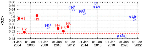
Figure 9.
Values of for each of the ‘precursory’ fluctuation minima on the date of of Table 1. The labels indicate whether they correspond to hit (H1 to H6, red bullets) or a false alarm (FA1 to FA6, blue circles). The dashed horizontal dashed red lines indicate the limits of Condition (14), i.e., 0.51 and 0.61, which when applied, validates all hits, while only FA1 and FA6 remain as false alarms.
We now turn to the statistical significance of the proposed method, which will be estimated by means of ROC, see Section 2.6. Our data, spanning from 1 January 1976 to the end of January 2022, consist of 553 months, which include 61 nine-month periods, plus an extra period of four months, which will be disregarded from the following calculations. The reason we choose a period of nine months is because, as already mentioned, the variability minima in the GCMT catalog have [13] a maximum lead time of nine months. Thus, we apply the ROC method by dividing the first 549-month period of the studied catalog into 61 nine-month periods so that . These periods, in our case, include only 6 EQs with , i.e., , a fact that translates to hit rate (we clarify that if we decrease the target threshold to 7.8, instead of 8.5, the hit rate would be lower than 100%, see also Appendix A of Sarlis et al. [13]). The false alarm rate, on the other hand, is equal to . Using the fortran code VISROC.f of Reference [121], we obtain in Figure 10, the ROC diagram where we depict, with the orange circle, the operation point that corresponds to our results, alongside the probability p to obtain this point by chance which is . If, however, we use the results after performing DFA and incorporating Condition (14), the false positive rate becomes equal to since we have only 2 false alarms. The corresponding ROC diagram is depicted in Figure 11. In this case, we have a p-value equal to . We should note that the two calculated p-values (i.e., and ) are comparable, since they are both of the order of , and in agreement with Reference [83], as well as the results obtained from a similar regional study of Japan [84,126]. Finally, Figure 10 and Figure 11 show that the AUC is close to 99%, when estimated by the k-ellipses, or 89% and 96% in the worst case scenario that the hit rate remains zero and abruptly increases to 100% at false positive rate 10.91% and 3.64%, respectively. Such values of AUC indicate excellent (>80%) or even outstanding (>90%) discrimination [127,128].
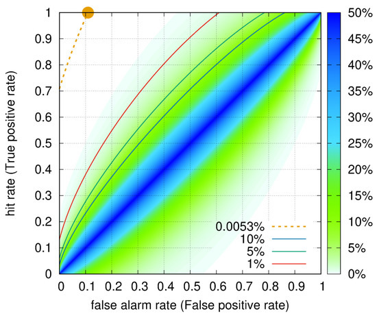
Figure 10.
Receiver Operating Characteristics diagram for and . The orange circle signifies the corresponding operation point and the orange dashed line the k-ellipse corresponding to . The colored contours represent the p-value to obtain by chance an ROC point based on the k-ellipses, with the darkest blue in the diagonal corresponding to random predictions. The k-ellipses with are also shown.
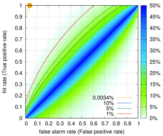
Figure 11.
Receiver Operating Characteristics diagram for the results after applying DFA. The orange circle signifies the corresponding operation point and the orange dashed line the k-ellipse corresponding to . The colored contours represent the p-value to obtain by chance an ROC point based on the k-ellipses, with the darkest blue in the diagonal corresponding to random predictions. The k-ellipses with are also shown.
5. Conclusions
We analyzed the Global Centroid Moment Tensor Catalog for the period 1 January 1976 until 31 January 2022. We employed natural time analysis of the order parameter of seismicity in order to identify the fluctuation minima that are precursory to EQs of , detrended fluctuation analysis for the identification of long-range correlations in the magnitude time series at the time of the minimum, and plot, at that time, the average earthquake potential score maps for providing information about the epicenter location. The results show that with statistical significance of the order of , the time of occurrence of the strongest EQs can be determined with a maximum lead time of nine months with outstanding discrimination, while their epicenters lie in a region covering 4% of the total studied area.
Author Contributions
Conceptualization, S.-R.G.C., E.S.S. and N.V.S.; methodology, S.-R.G.C., P.K.V., J.P.-O., E.S.S. and N.V.S.; software, S.-R.G.C., J.P.-O., E.S.S. and N.V.S.; validation, P.K.V., J.P.-O., K.A.P. and E.S.S.; formal analysis, S.-R.G.C. and N.V.S.; investigation, S.-R.G.C., P.K.V., J.P.-O., K.A.P., E.S.S. and N.V.S.; resources, S.-R.G.C., E.S.S. and N.V.S.; data curation, E.S.S. and N.V.S.; writing—original draft preparation, S.-R.G.C., P.K.V., J.P.-O., K.A.P., E.S.S. and N.V.S.; writing—review and editing, S.-R.G.C., P.K.V., J.P.-O., K.A.P., E.S.S. and N.V.S.; visualization, S.-R.G.C., K.A.P., E.S.S. and N.V.S.; supervision, S.-R.G.C. and N.V.S.; project administration, N.V.S. All authors have read and agreed to the published version of the manuscript.
Funding
This research received no external funding.
Data Availability Statement
Earthquake data come from the GCMT project [89,90], all catalogs can be found in the home page http://www.globalcmt.org/CMTfiles.html (accessed on 23 May 2022). Gnuplot [129] was used for the preparation of Figure 2, Figure 3, Figure 4, Figure 5, Figure 6, Figure 7, Figure 8 and Figure 9 and the coast lines were imported from GEODAS Coastline Extractor [130]. ETOPO1 Global Relief Model [91] was used to integrate the land topography and ocean bathymetry in Figure 1. In particular, the ETOPO1 Ice Surface Grid Version is chosen, which also depicts the top of the Antarctic and Greenland ice sheets. It is publicly available at the https://www.ngdc.noaa.gov/mgg/global/ (accessed on 24 June 2022). For the color scale, the palete ETOPO1-Reed was used, which is publicly available at http://soliton.vm.bytemark.co.uk/pub/cpt-city/ngdc/index.html (accessed on 24 June 2022). The datasets generated and/or analyzed during the current study are available from the corresponding author on reasonable request.
Conflicts of Interest
The authors declare no conflict of interest.
References
- Varotsos, P.A.; Sarlis, N.V.; Skordas, E.S. Spatio-Temporal complexity aspects on the interrelation between Seismic Electric Signals and Seismicity. Pract. Athens Acad. 2001, 76, 294–321. [Google Scholar]
- Varotsos, P.A.; Sarlis, N.V.; Skordas, E.S. Long-range correlations in the electric signals that precede rupture. Phys. Rev. E 2002, 66, 011902. [Google Scholar] [CrossRef] [PubMed] [Green Version]
- Varotsos, P.A.; Sarlis, N.V.; Skordas, E.S. Seismic Electric Signals and Seismicity: On a tentative interrelation between their spectral content. Acta Geophys. Pol. 2002, 50, 337–354. [Google Scholar]
- Varotsos, P.A.; Sarlis, N.V.; Skordas, E.S. Natural Time Analysis: The new view of time. Precursory Seismic Electric Signals, Earthquakes and other Complex Time-Series; Springer: Berlin/Heidelberg, Germany, 2011. [Google Scholar] [CrossRef]
- Varotsos, P.A.; Sarlis, N.V.; Tanaka, H.K.; Skordas, E.S. Similarity of fluctuations in correlated systems: The case of seismicity. Phys. Rev. E 2005, 72, 041103. [Google Scholar] [CrossRef] [PubMed] [Green Version]
- Varotsos, P.A.; Sarlis, N.V.; Skordas, E.S.; Lazaridou, M.S. Fluctuations, under time reversal, of the natural time and the entropy distinguish similar looking electric signals of different dynamics. J. Appl. Phys. 2008, 103, 014906. [Google Scholar] [CrossRef] [Green Version]
- Sarlis, N.V.; Skordas, E.S.; Lazaridou, M.S.; Varotsos, P.A. Investigation of seismicity after the initiation of a Seismic Electric Signal activity until the main shock. Proc. Jpn. Acad. Ser. B Phys. Biol. Sci. 2008, 84, 331–343. [Google Scholar] [CrossRef]
- Uyeda, S.; Kamogawa, M. The Prediction of Two Large Earthquakes in Greece. Eos Trans. AGU 2008, 89, 363. [Google Scholar] [CrossRef]
- Uyeda, S.; Kamogawa, M. Comment on ‘The Prediction of Two Large Earthquakes in Greece’. Eos Trans. AGU 2010, 91, 163. [Google Scholar] [CrossRef]
- Varotsos, P.A.; Sarlis, N.V.; Skordas, E.S.; Uyeda, S.; Kamogawa, M. Natural time analysis of critical phenomena. Proc. Natl. Acad. Sci. USA 2011, 108, 11361–11364. [Google Scholar] [CrossRef] [Green Version]
- Sarlis, N.V.; Skordas, E.S.; Varotsos, P.A.; Nagao, T.; Kamogawa, M.; Tanaka, H.; Uyeda, S. Minimum of the order parameter fluctuations of seismicity before major earthquakes in Japan. Proc. Natl. Acad. Sci. USA 2013, 110, 13734–13738. [Google Scholar] [CrossRef] [Green Version]
- Sarlis, N.V.; Skordas, E.S.; Varotsos, P.A.; Nagao, T.; Kamogawa, M.; Uyeda, S. Spatiotemporal variations of seismicity before major earthquakes in the Japanese area and their relation with the epicentral locations. Proc. Natl. Acad. Sci. USA 2015, 112, 986–989. [Google Scholar] [CrossRef] [PubMed] [Green Version]
- Sarlis, N.V.; Christopoulos, S.R.G.; Skordas, E.S. Minima of the fluctuations of the order parameter of global seismicity. Chaos 2015, 25, 063110. [Google Scholar] [CrossRef] [PubMed] [Green Version]
- Sarlis, N.V.; Skordas, E.S.; Varotsos, P.A. A remarkable change of the entropy of seismicity in natural time under time reversal before the super-giant M9 Tohoku earthquake on 11 March 2011. EPL Europhys. Lett. 2018, 124, 29001. [Google Scholar] [CrossRef]
- Varotsos, P.A.; Sarlis, N.V.; Skordas, E.S.; Lazaridou, M.S. Identifying sudden cardiac death risk and specifying its occurrence time by analyzing electrocardiograms in natural time. Appl. Phys. Lett. 2007, 91, 064106. [Google Scholar] [CrossRef]
- Baldoumas, G.; Peschos, D.; Tatsis, G.; Christofilakis, V.; Chronopoulos, S.K.; Kostarakis, P.; Varotsos, P.A.; Sarlis, N.V.; Skordas, E.S.; Bechlioulis, A.; et al. Remote sensing natural time analysis of heartbeat data by means of a portable photoplethysmography device. Int. J. Remote Sens. 2021, 42, 2292–2302. [Google Scholar] [CrossRef]
- Tsuji, D.; Katsuragi, H. Temporal analysis of acoustic emission from a plunged granular bed. Phys. Rev. E 2015, 92, 042201. [Google Scholar] [CrossRef] [PubMed] [Green Version]
- Ferre, J.; Barzegar, A.; Katzgraber, H.G.; Scalettar, R. Distribution of interevent avalanche times in disordered and frustrated spin systems. Phys. Rev. B 2019, 99, 024411. [Google Scholar] [CrossRef] [Green Version]
- Loukidis, A.; Perez-Oregon, J.; Pasiou, E.D.; Sarlis, N.V.; Triantis, D. Similarity of fluctuations in critical systems: Acoustic emissions observed before fracture. Physica A 2020, 566, 125622. [Google Scholar] [CrossRef]
- Ramírez-Rojas, A.; Telesca, L.; Angulo-Brown, F. Entropy of geoelectrical time series in the natural time domain. Nat. Hazards Earth Syst. Sci. 2011, 11, 219–225. [Google Scholar] [CrossRef]
- Potirakis, S.M.; Karadimitrakis, A.; Eftaxias, K. Natural time analysis of critical phenomena: The case of pre-fracture electromagnetic emissions. Chaos 2013, 23, 023117. [Google Scholar] [CrossRef]
- Vallianatos, F.; Michas, G.; Benson, P.; Sammonds, P. Natural time analysis of critical phenomena: The case of acoustic emissions in triaxially deformed Etna basalt. Physica A 2013, 392, 5172–5178. [Google Scholar] [CrossRef]
- Vallianatos, F.; Michas, G.; Papadakis, G. Non-extensive and natural time analysis of seismicity before the Mw6.4, 12 October 2013 earthquake in the South West segment of the Hellenic Arc. Physica A 2014, 414, 163–173. [Google Scholar] [CrossRef]
- Potirakis, S.M.; Eftaxias, K.; Schekotov, A.; Yamaguchi, H.; Hayakawa, M. Criticality features in ultra-low frequency magnetic fields prior to the 2013 M6.3 Kobe earthquake. Ann. Geophys. 2016, 59, S0317. [Google Scholar] [CrossRef]
- Potirakis, S.M.; Asano, T.; Hayakawa, M. Criticality Analysis of the Lower Ionosphere Perturbations Prior to the 2016 Kumamoto (Japan) Earthquakes as Based on VLF Electromagnetic Wave Propagation Data Observed at Multiple Stations. Entropy 2018, 20, 199. [Google Scholar] [CrossRef] [PubMed] [Green Version]
- Ramírez-Rojas, A.; Flores-Márquez, E.L.; Sarlis, N.V.; Varotsos, P.A. The Complexity Measures Associated with the Fluctuations of the Entropy in Natural Time before the Deadly Mexico M8.2 Earthquake on 7 September 2017. Entropy 2018, 20, 477. [Google Scholar] [CrossRef] [Green Version]
- Yang, S.S.; Potirakis, S.M.; Sasmal, S.; Hayakawa, M. Natural Time Analysis of Global Navigation Satellite System Surface Deformation: The Case of the 2016 Kumamoto Earthquakes. Entropy 2020, 22, 674. [Google Scholar] [CrossRef]
- Vallianatos, F.; Michas, G.; Hloupis, G. Seismicity Patterns Prior to the Thessaly (Mw6.3) Strong Earthquake on 3 March 2021 in Terms of Multiresolution Wavelets and Natural Time Analysis. Geosciences 2021, 11, 379. [Google Scholar] [CrossRef]
- Hloupis, G.; Stavrakas, I.; Vallianatos, F.; Triantis, D. A preliminary study for prefailure indicators in acoustic emissions using wavelets and natural time analysis. Proc. Inst. Mech. Eng. Part J. Mater. Des. Appl. 2016, 230, 780–788. [Google Scholar] [CrossRef]
- Niccolini, G.; Lacidogna, G.; Carpinteri, A. Fracture precursors in a working girder crane: AE natural-time and b-value time series analyses. Eng. Fract. Mech. 2019, 210, 393–399. [Google Scholar] [CrossRef]
- Loukidis, A.; Pasiou, E.D.; Sarlis, N.V.; Triantis, D. Fracture analysis of typical construction materials in natural time. Physica A 2019, 547, 123831. [Google Scholar] [CrossRef]
- Baldoumas, G.; Peschos, D.; Tatsis, G.; Chronopoulos, S.K.; Christofilakis, V.; Kostarakis, P.; Varotsos, P.; Sarlis, N.V.; Skordas, E.S.; Bechlioulis, A.; et al. A Prototype Photoplethysmography Electronic Device that Distinguishes Congestive Heart Failure from Healthy Individuals by Applying Natural Time Analysis. Electronics 2019, 8, 1288. [Google Scholar] [CrossRef] [Green Version]
- Niccolini, G.; Potirakis, S.M.; Lacidogna, G.; Borla, O. Criticality Hidden in Acoustic Emissions and in Changing Electrical Resistance during Fracture of Rocks and Cement-Based Materials. Materials 2020, 13, 5608. [Google Scholar] [CrossRef] [PubMed]
- Loukidis, A.; Triantis, D.; Stavrakas, I.; Pasiou, E.D.; Kourkoulis, S.K. Detecting Criticality by Exploring the Acoustic Activity in Terms of the “Natural-Time” Concept. Appl. Sci. 2022, 12, 231. [Google Scholar] [CrossRef]
- Kourkoulis, S.K.; Pasiou, E.D.; Loukidis, A.; Stavrakas, I.; Triantis, D. Comparative Assessment of Criticality Indices Extracted from Acoustic and Electrical Signals Detected in Marble Specimens. Infrastructures 2022, 7, 15. [Google Scholar] [CrossRef]
- Friedrich, L.F.; Cezar, E.S.; Colpo, A.B.; Tanzi, B.N.R.; Sobczyk, M.; Lacidogna, G.; Niccolini, G.; Kosteski, L.E.; Iturrioz, I. Long-Range Correlations and Natural Time Series Analyses from Acoustic Emission Signals. Appl. Sci. 2022, 12, 1980. [Google Scholar] [CrossRef]
- Varotsos, C.A.; Tzanis, C. A new tool for the study of the ozone hole dynamics over Antarctica. Atmos. Environ. 2012, 47, 428–434. [Google Scholar] [CrossRef]
- Varotsos, C.A.; Tzanis, C.; Cracknell, A.P. Precursory signals of the major El Niño Southern Oscillation events. Theor. Appl. Climatol. 2016, 124, 903–912. [Google Scholar] [CrossRef]
- Varotsos, C.A.; Tzanis, C.G.; Sarlis, N.V. On the progress of the 2015–2016 El Niño event. Atmos. Chem. Phys. Discuss. 2015, 15, 35787–35797. [Google Scholar] [CrossRef] [Green Version]
- Varotsos, C.A.; Sarlis, N.V.; Efstathiou, M. On the association between the recent episode of the quasi-biennial oscillation and the strong El Niño event. Theor. Appl. Climatol. 2018, 133, 569–577. [Google Scholar] [CrossRef]
- Varotsos, C.A.; Golitsyn, G.S.; Efstathiou, M.; Sarlis, N. A new method of nowcasting extreme cosmic ray events. Remote. Sens. Lett. 2022. [Google Scholar] [CrossRef]
- Rundle, J.B.; Turcotte, D.L.; Donnellan, A.; Grant Ludwig, L.; Luginbuhl, M.; Gong, G. Nowcasting earthquakes. Earth Space Sci. 2016, 3, 480–486. [Google Scholar] [CrossRef]
- Rundle, J.B.; Luginbuhl, M.; Giguere, A.; Turcotte, D.L. Natural Time, Nowcasting and the Physics of Earthquakes: Estimation of Seismic Risk to Global Megacities. Pure Appl. Geophys. 2018, 175, 647–660. [Google Scholar] [CrossRef] [Green Version]
- Luginbuhl, M.; Rundle, J.B.; Hawkins, A.; Turcotte, D.L. Nowcasting Earthquakes: A Comparison of Induced Earthquakes in Oklahoma and at the Geysers, California. Pure Appl. Geophys. 2018, 175, 49–65. [Google Scholar] [CrossRef]
- Luginbuhl, M.; Rundle, J.B.; Turcotte, D.L. Natural Time and Nowcasting Earthquakes: Are Large Global Earthquakes Temporally Clustered? Pure Appl. Geophys. 2018, 175, 661–670. [Google Scholar] [CrossRef]
- Rundle, J.B.; Donnellan, A. Nowcasting Earthquakes in Southern California With Machine Learning: Bursts, Swarms, and Aftershocks May Be Related to Levels of Regional Tectonic Stress. Earth Space Sci. 2020, 7, e2020EA001097. [Google Scholar] [CrossRef]
- Rundle, J.; Stein, S.; Donnellan, A.; Turcotte, D.L.; Klein, W.; Saylor, C. The Complex Dynamics of Earthquake Fault Systems: New Approaches to Forecasting and Nowcasting of Earthquakes. Rep. Prog. Phys. 2021, 84, 076801. [Google Scholar] [CrossRef]
- Rundle, J.B.; Donnellan, A.; Fox, G.; Crutchfield, J.P. Nowcasting Earthquakes by Visualizing the Earthquake Cycle with Machine Learning: A Comparison of Two Methods. Surv. Geophys. 2022, 43, 483–501. [Google Scholar] [CrossRef]
- Rundle, J.B.; Donnellan, A.; Fox, G.; Crutchfield, J.P.; Granat, R. Nowcasting Earthquakes:Imaging the Earthquake Cycle in California with Machine Learning. Earth Space Sci. 2021, 8, e2021EA001757. [Google Scholar] [CrossRef]
- Fildes, R.A.; Turcotte, D.L.; Rundle, J.B. Natural time analysis and nowcasting of quasi-periodic collapse events during the 2018 Kīlauea volcano eruptive sequence. Earth Space Sci. 2022, 9, e2022EA002266. [Google Scholar] [CrossRef]
- Sarlis, N.V.; Skordas, E.S.; Varotsos, P.A. Multiplicative cascades and seismicity in natural time. Phys. Rev. E 2009, 80, 022102. [Google Scholar] [CrossRef] [Green Version]
- Sarlis, N.V.; Christopoulos, S.R.G. Natural time analysis of the Centennial Earthquake Catalog. Chaos 2012, 22, 023123. [Google Scholar] [CrossRef] [PubMed]
- Ramírez-Rojas, A.; Flores-Márquez, E. Order parameter analysis of seismicity of the Mexican Pacific coast. Physica A 2013, 392, 2507–2512. [Google Scholar] [CrossRef]
- Flores-Márquez, E.; Vargas, C.; Telesca, L.; Ramírez-Rojas, A. Analysis of the distribution of the order parameter of synthetic seismicity generated by a simple spring-block system with asperities. Physica A 2014, 393, 508–512. [Google Scholar] [CrossRef]
- Sarlis, N.V.; Skordas, E.S.; Varotsos, P.A.; Ramírez-Rojas, A.; Flores-Márquez, E.L. Natural Time Analysis: On the Deadly Mexico M8.2 Earthquake on 7 September 2017. Physica A 2018, 506, 625–634. [Google Scholar] [CrossRef]
- Sarlis, N.V.; Skordas, E.S.; Varotsos, P.A. Similarity of fluctuations in systems exhibiting Self-Organized Criticality. EPL 2011, 96, 28006. [Google Scholar] [CrossRef]
- Olami, Z.; Feder, H.J.S.; Christensen, K. Self-organized criticality in a continuous, nonconservative cellular automaton modeling earthquakes. Phys. Rev. Lett. 1992, 68, 1244–1247. [Google Scholar] [CrossRef] [Green Version]
- Sarlis, N.V.; Skordas, E.S.; Varotsos, P.A. The change of the entropy in natural time under time-reversal in the Olami-Feder-Christensen earthquake model. Tectonophysics 2011, 513, 49–53. [Google Scholar] [CrossRef]
- Burridge, R.; Knopoff, L. Model and theoretical seismicity. Bull. Seismol. Soc. Am. 1967, 57, 341–371. [Google Scholar] [CrossRef]
- Varotsos, P.A.; Sarlis, N.V.; Skordas, E.S.; Uyeda, S.; Kamogawa, M. Natural time analysis of critical phenomena. The case of Seismicity. EPL 2010, 92, 29002. [Google Scholar] [CrossRef] [Green Version]
- Sarlis, N.V.; Skordas, E.S.; Varotsos, P.A. Order parameter fluctuations of seismicity in natural time before and after mainshocks. EPL 2010, 91, 59001. [Google Scholar] [CrossRef] [Green Version]
- Varotsos, P.A.; Sarlis, N.V.; Skordas, E.S. Natural time analysis: Important changes of the order parameter of seismicity preceding the 2011 M9 Tohoku earthquake in Japan. EPL Europhys. Lett. 2019, 125, 69001. [Google Scholar] [CrossRef] [Green Version]
- Varotsos, P.A.; Sarlis, N.V.; Skordas, E.S. Remarkable changes in the distribution of the order parameter of seismicity before mainshocks. EPL 2012, 100, 39002. [Google Scholar] [CrossRef] [Green Version]
- Varotsos, P.A.; Sarlis, N.V.; Skordas, E.S. Order parameter fluctuations in natural time and b-value variation before large earthquakes. Nat. Hazards Earth Syst. Sci. 2012, 12, 3473–3481. [Google Scholar] [CrossRef] [Green Version]
- Varotsos, P.A.; Sarlis, N.V.; Skordas, E.S. Scale-specific order parameter fluctuations of seismicity in natural time before mainshocks. EPL 2011, 96, 59002. [Google Scholar] [CrossRef] [Green Version]
- Varotsos, P.; Alexopoulos, K. Thermodynamics of Point Defects and their Relation with Bulk Properties; North Holland: Amsterdam, The Netherlands, 1986. [Google Scholar]
- Varotsos, P.; Lazaridou, M. Latest aspects of earthquake prediction in Greece based on Seismic Electric Signals. Tectonophysics 1991, 188, 321–347. [Google Scholar] [CrossRef]
- Varotsos, P.; Alexopoulos, K.; Lazaridou, M. Latest aspects of earthquake prediction in Greece based on Seismic Electric Signals, II. Tectonophysics 1993, 224, 1–37. [Google Scholar] [CrossRef] [Green Version]
- Uyeda, S.; Nagao, T.; Orihara, Y.; Yamaguchi, T.; Takahashi, I. Geoelectric potential changes: Possible precursors to earthquakes in Japan. Proc. Natl. Acad. Sci. USA 2000, 97, 4561–4566. [Google Scholar] [CrossRef] [Green Version]
- Uyeda, S.; Hayakawa, M.; Nagao, T.; Molchanov, O.; Hattori, K.; Orihara, Y.; Gotoh, K.; Akinaga, Y.; Tanaka, H. Electric and magnetic phenomena observed before the volcano-seismic activity in 2000 in the Izu Island Region, Japan. Proc. Natl. Acad. Sci. USA 2002, 99, 7352–7355. [Google Scholar] [CrossRef] [Green Version]
- Uyeda, S.; Kamogawa, M.; Tanaka, H. Analysis of electrical activity and seismicity in the natural time domain for the volcanic-seismic swarm activity in 2000 in the Izu Island region, Japan. J. Geophys. Res. 2009, 114, B02310. [Google Scholar] [CrossRef] [Green Version]
- Uyeda, S.; Nagao, T.; Kamogawa, M. Short-term earthquake prediction: Current status of seismo-electromagnetics. Tectonophysics 2009, 470, 205–213. [Google Scholar] [CrossRef]
- Varotsos, P. The Physics of Seismic Electric Signals; TERRAPUB: Tokyo, Japan, 2005; p. 338. [Google Scholar]
- Sarlis, N.V. Statistical Significance of Earth’s Electric and Magnetic Field Variations Preceding Earthquakes in Greece and Japan Revisited. Entropy 2018, 20, 561. [Google Scholar] [CrossRef] [Green Version]
- Varotsos, P.A.; Sarlis, N.V.; Skordas, E.S. Phenomena preceding major earthquakes interconnected through a physical model. Ann. Geophys. 2019, 37, 315–324. [Google Scholar] [CrossRef] [Green Version]
- Varotsos, P.; Sarlis, N.; Skordas, E. Scale-specific order parameter fluctuations of seismicity before mainshocks: Natural time and Detrended Fluctuation Analysis. EPL 2012, 99, 59001. [Google Scholar] [CrossRef]
- Sarlis, N.V.; Skordas, E.S.; Varotsos, P.A.; Ramírez-Rojas, A.; Flores-Márquez, E.L. Identifying the Occurrence Time of the Deadly Mexico M8.2 Earthquake on 7 September 2017. Entropy 2019, 21, 301. [Google Scholar] [CrossRef] [Green Version]
- Flores-Márquez, E.L.; Ramírez-Rojas, A.; Perez-Oregon, J.; Sarlis, N.V.; Skordas, E.S.; Varotsos, P.A. Natural Time Analysis of Seismicity within the Mexican Flat Slab before the M7.1 Earthquake on 19 September 2017. Entropy 2020, 22, 730. [Google Scholar] [CrossRef] [PubMed]
- Perez-Oregon, J.; Varotsos, P.K.; Skordas, E.S.; Sarlis, N.V. Estimating the Epicenter of a Future Strong Earthquake in Southern California, Mexico, and Central America by Means of Natural Time Analysis and Earthquake Nowcasting. Entropy 2021, 23, 1658. [Google Scholar] [CrossRef]
- Mintzelas, A.; Sarlis, N. Minima of the fluctuations of the order parameter of seismicity and earthquake networks based on similar activity patterns. Physica A 2019, 527, 121293. [Google Scholar] [CrossRef]
- Varotos, P.K.; Perez-Oregon, J.; Skordas, E.S.; Sarlis, N.V. Estimating the epicenter of an impending strong earthquake by combining the seismicity order parameter variability analysis with earthquake networks and nowcasting: Application in Eastern Mediterranean. Appl. Sci. 2021, 11, 10093. [Google Scholar] [CrossRef]
- Sarlis, N.V.; Skordas, E.S.; Mintzelas, A.; Papadopoulou, K.A. Micro-scale, mid-scale, and macro-scale in global seismicity identified by empirical mode decomposition and their multifractal characteristics. Sci. Rep. 2018, 8, 9206. [Google Scholar] [CrossRef]
- Christopoulos, S.R.G.; Skordas, E.S.; Sarlis, N.V. On the Statistical Significance of the Variability Minima of the Order Parameter of Seismicity by Means of Event Coincidence Analysis. Appl. Sci. 2020, 10, 662. [Google Scholar] [CrossRef] [Green Version]
- Sarlis, N.V.; Skordas, E.S.; Christopoulos, S.R.G.; Varotsos, P.A. Natural Time Analysis: The Area under the Receiver Operating Characteristic Curve of the Order Parameter Fluctuations Minima Preceding Major Earthquakes. Entropy 2020, 22, 583. [Google Scholar] [CrossRef] [PubMed]
- Varotsos, P.A.; Sarlis, N.V.; Skordas, E.S.; Lazaridou, M.S. Seismic Electric Signals: An additional fact showing their physical interconnection with seismicity. Tectonophysics 2013, 589, 116–125. [Google Scholar] [CrossRef]
- Varotsos, P.A.; Sarlis, N.V.; Skordas, E.S. Study of the temporal correlations in the magnitude time series before major earthquakes in Japan. J. Geophys. Res. Space Phys. 2014, 119, 9192–9206. [Google Scholar] [CrossRef]
- Sarlis, N.V.; Skordas, E.S.; Varotsos, P.A.; Ramírez-Rojas, A.; Flores-Márquez, E.L. Investigation of the temporal correlations between earthquake magnitudes before the Mexico M8.2 earthquake on 7 September 2017. Physica A 2019, 517, 475–483. [Google Scholar] [CrossRef]
- Varotsos, P.A.; Sarlis, N.V.; Skordas, E.S. Order Parameter and Entropy of Seismicity in Natural Time before Major Earthquakes: Recent Results. Geosciences 2022, 12, 225. [Google Scholar] [CrossRef]
- Dziewoński, A.M.; Chou, T.A.; Woodhouse, J.H. Determination of earthquake source parameters from waveform data for studies of global and regional seismicity. J. Geophys. Res. Solid Earth 1981, 86, 2825–2852. [Google Scholar] [CrossRef]
- Ekström, G.; Nettles, M.; Dziewoński, A. The global CMT project 2004-2010: Centroid-moment tensors for 13,017 earthquakes. Phys. Earth Planet. Inter. 2012, 200–201, 1–9. [Google Scholar] [CrossRef]
- Amante, C.; Eakins, B.W. ETOPO1 1 Arc-Minute Global Relief Model: Procedures, Data Sources and Analysis. NOAA Technical Memorandum NESDIS NGDC-24; National Geophysical Data Center, Marine Geology and Geophysics Division: Boulder, CO, Canada, 2009. [Google Scholar] [CrossRef]
- Wessel, P.; Luis, J.F.; Uieda, L.; Scharroo, R.; Wobbe, F.; Smith, W.H.F.; Tian, D. The Generic Mapping Tools Version 6. Geochem. Geophys. Geosyst. 2019, 20, 5556–5564. [Google Scholar] [CrossRef] [Green Version]
- Wiemer, S. A Software Package to Analyze Seismicity: ZMAP. Seismol. Res. Lett. 2001, 72, 373–382. [Google Scholar] [CrossRef]
- Kanamori, H. Quantification of Earthquakes. Nature 1978, 271, 411–414. [Google Scholar] [CrossRef]
- Tanaka, H.K.; Varotsos, P.A.; Sarlis, N.V.; Skordas, E.S. A plausible universal behaviour of earthquakes in the natural time-domain. Proc. Jpn. Acad. Ser. B Phys. Biol. Sci. 2004, 80, 283–289. [Google Scholar] [CrossRef] [Green Version]
- Peng, C.K.; Buldyrev, S.V.; Havlin, S.; Simons, M.; Stanley, H.E.; Goldberger, A.L. Mosaic organization of DNA nucleotides. Phys. Rev. E 1994, 49, 1685–1689. [Google Scholar] [CrossRef] [PubMed] [Green Version]
- Mantegna, R.N.; Buldyrev, S.V.; Goldberger, A.L.; Havlin, S.; Peng, C.K.; Simons, M.; Stanley, H.E. Linguistic Features of Noncoding DNA Sequences. Phys. Rev. Lett. 1994, 73, 3169–3172. [Google Scholar] [CrossRef]
- Buldyrev, S.V.; Goldberger, A.L.; Havlin, S.; Mantegna, R.N.; Matsa, M.E.; Peng, C.K.; Simons, M.; Stanley, H.E. Long-range correlation properties of coding and noncoding DNA sequences: GenBank analysis. Phys. Rev. E 1995, 51, 5084–5091. [Google Scholar] [CrossRef] [PubMed]
- Ivanov, P.C.; Rosenblum, M.G.; Peng, C.K.; Mietus, J.; Havlin, S.; Stanley, H.E.; Goldberger, A.L. Multifractality in human heartbeat dynamics. Nature 1999, 399, 461. [Google Scholar] [CrossRef] [Green Version]
- Havlin, S.; Buldyrev, S.V.; Bunde, A.; Goldberger, A.L.; Ivanov, P.C.; Peng, C.K.; Stanley, H.E. Scaling in nature: From DNA through heartbeats to weather. Physica A 1999, 273, 46–69. [Google Scholar] [CrossRef]
- Stanley, H.E.; Amaral, L.A.N.; Goldberger, A.L.; Havlin, S.; Ivanov, P.C.; Peng, C.K. Statistical physics and physiology: Monofractal and multifractal approaches. Physica A 1999, 270, 309–324. [Google Scholar] [CrossRef]
- Hardstone, R.; Poil, S.S.; Schiavone, G.; Jansen, R.; Nikulin, V.; Mansvelder, H.; Linkenkaer-Hansen, K. Detrended Fluctuation Analysis: A Scale-Free View on Neuronal Oscillations. Front. Physiol. 2012, 3, 450. [Google Scholar] [CrossRef] [Green Version]
- Bunde, A.; Havlin, S.; Kantelhardt, J.W.; Penzel, T.; Peter, J.H.; Voigt, K. Correlated and Uncorrelated Regions in Heart-Rate Fluctuations during Sleep. Phys. Rev. Lett. 2000, 85, 3736–3739. [Google Scholar] [CrossRef] [Green Version]
- Ivanov, P.C.; Nunes Amaral, L.A.; Goldberger, A.L.; Stanley, H.E. Stochastic feedback and the regulation of biological rhythms. Europhys. Lett. 1998, 43, 363–368. [Google Scholar] [CrossRef] [Green Version]
- Ivanova, K.; Ackerman, T.P.; Clothiaux, E.E.; Ivanov, P.C.; Stanley, H.E.; Ausloos, M. Time correlations and 1/f behavior in backscattering radar reflectivity measurements from cirrus cloud ice fluctuations. J. Geophys. Res. Atmos. 2003, 108 D9, 4268. [Google Scholar] [CrossRef]
- Peng, C.K.; Buldyrev, S.V.; Goldberger, A.L.; Havlin, S.; Mantegna, R.N.; Simons, M.; Stanley, H.E. Statistical properties of DNA sequences. Physica A 1995, 221, 180–192. [Google Scholar] [CrossRef]
- Goldberger, A.L.; Amaral, L.A.N.; Glass, L.; Hausdorff, J.M.; Ivanov, P.C.; Mark, R.G.; Mictus, J.E.; Moody, G.B.; Peng, C.K.; Stanley, H.E. PhysioBank, PhysioToolkit, and PhysioNet - Components of a new research resource for complex physiologic signals. Circulation 2000, 101, E215. [Google Scholar] [CrossRef] [PubMed] [Green Version]
- Sarlis, N.V.; Skordas, E.S. Study in Natural Time of Geoelectric Field and Seismicity Changes Preceding the Mw6.8 Earthquake on 25 October 2018 in Greece. Entropy 2018, 20, 882. [Google Scholar] [CrossRef] [Green Version]
- Pasari, S. Nowcasting Earthquakes in the Bay of Bengal Region. Pure Appl. Geophys. 2019, 176, 1417–1432. [Google Scholar] [CrossRef]
- Pasari, S.; Sharma, Y. Contemporary Earthquake Hazards in the West-Northwest Himalaya: A Statistical Perspective through Natural Times. Seismol. Res. Lett. 2020, 91, 3358–3369. [Google Scholar] [CrossRef]
- Perez-Oregon, J.; Angulo-Brown, F.; Sarlis, N.V. Nowcasting Avalanches as Earthquakes and the Predictability of Strong Avalanches in the Olami-Feder-Christensen Model. Entropy 2020, 22, 1228. [Google Scholar] [CrossRef]
- Pasari, S.; Simanjuntak, A.V.H.; Neha.; Sharma, Y. Nowcasting earthquakes in Sulawesi Island, Indonesia. Geosci. Lett. 2021, 8, 27. [Google Scholar] [CrossRef]
- Sarlis, N.V. Magnitude correlations in global seismicity. Phys. Rev. E 2011, 84, 022101. [Google Scholar] [CrossRef]
- Ferguson, C.D.; Klein, W.; Rundle, J.B. Spinodals, scaling, and ergodicity in a threshold model with long-range stress transfer. Phys. Rev. E 1999, 60, 1359–1373. [Google Scholar] [CrossRef]
- Tiampo, K.F.; Rundle, J.B.; Klein, W.; Martins, J.S.S.; Ferguson, C.D. Ergodic Dynamics in a Natural Threshold System. Phys. Rev. Lett. 2003, 91, 238501. [Google Scholar] [CrossRef] [Green Version]
- Tiampo, K.F.; Rundle, J.B.; Klein, W.; Holliday, J.; Sá Martins, J.S.; Ferguson, C.D. Ergodicity in natural earthquake fault networks. Phys. Rev. E 2007, 75, 066107. [Google Scholar] [CrossRef] [PubMed] [Green Version]
- Press, W.H.; Teukolsky, S.; Vettrling, W.; Flannery, B.P. Numerical Recipes in FORTRAN; Cambridge Univrsity Press: New York, NY, USA, 1992; p. 963. [Google Scholar]
- Fawcett, T. An introduction to ROC analysis. Pattern Recogn. Lett. 2006, 27, 861–874. [Google Scholar] [CrossRef]
- Mason, S.J.; Graham, N.E. Areas beneath the relative operating characteristics (ROC) and relative operating levels (ROL) curves: Statistical significance and interpretation. Quart. J. Roy. Meteor. Soc. 2002, 128, 2145–2166. [Google Scholar] [CrossRef]
- Mann, H.B.; Whitney, D.R. On a Test of Whether one of Two Random Variables is Stochastically Larger than the Other. Ann. Math. Statist. 1947, 18, 50–60. [Google Scholar] [CrossRef]
- Sarlis, N.V.; Christopoulos, S.R.G. Visualization of the significance of Receiver Operating Characteristics based on confidence ellipses. Comput. Phys. Commun. 2014, 185, 1172–1176. [Google Scholar] [CrossRef] [Green Version]
- Bak, P.; Christensen, K.; Danon, L.; Scanlon, T. Unified Scaling Law for Earthquakes. Phys. Rev. Lett. 2002, 88, 178501. [Google Scholar] [CrossRef] [Green Version]
- Liu, C.; Lay, T.; Xiong, X.; Wen, Y. Rupture of the 2020 MW 7.8 Earthquake in the Shumagin Gap Inferred From Seismic and Geodetic Observations. Geophys. Res. Lett. 2020, 47, e2020GL090806. [Google Scholar] [CrossRef]
- Elliott, J.L.; Grapenthin, R.; Parameswaran, R.M.; Xiao, Z.; Freymueller, J.T.; Fusso, L. Cascading rupture of a megathrust. Sci. Adv. 2022, 8, eabm4131. [Google Scholar] [CrossRef] [PubMed]
- Liu, C.; Lay, T.; Xiong, X. The 29 July 2021 MW 8.2 Chignik, Alaska Peninsula Earthquake Rupture Inferred From Seismic and Geodetic Observations: Re-Rupture of the Western 2/3 of the 1938 Rupture Zone. Geophys. Res. Lett. 2022, 49, e2021GL096004. [Google Scholar] [CrossRef]
- Sarlis, N.V.; Skordas, E.S.; Christopoulos, S.R.G.; Varotsos, P.A. Statistical Significance of Minimum of the Order Parameter Fluctuations of Seismicity Before Major Earthquakes in Japan. Pure Appl. Geophys. 2016, 173, 165–172. [Google Scholar] [CrossRef] [Green Version]
- Hosmer, D.W.; Lemeshow, S. Applied Logistic Regression; John Wiley & Sons, Ltd: New York, NY, USA, 2000. [Google Scholar] [CrossRef]
- Mandrekar, J.N. Receiver Operating Characteristic Curve in Diagnostic Test Assessment. J. Thorac. Oncol. 2010, 5, 1315–1316. [Google Scholar] [CrossRef] [PubMed] [Green Version]
- Williams, T.; Kelley, C. Gnuplot 4.6: An Interactive Plotting Program, 2014. Available online: http://www.gnuplot.info (accessed on 28 February 2014).
- Metzger, D.R. GEODAS Coastline Extractor, Version 1.1.3.1. 2014. Available online: http://www.ngdc.noaa.gov/mgg/dat/geodas/software/mswindows/geodas-ng_setup.exe (accessed on 11 February 2015).
Publisher’s Note: MDPI stays neutral with regard to jurisdictional claims in published maps and institutional affiliations. |
© 2022 by the authors. Licensee MDPI, Basel, Switzerland. This article is an open access article distributed under the terms and conditions of the Creative Commons Attribution (CC BY) license (https://creativecommons.org/licenses/by/4.0/).