Numerical Simulation of Non-Isothermal Mixing Flow Characteristics with ELES Method

Abstract

Thermal fatigue caused by turbulent thermal mixing in tee pipes is always one of the failure factors of industrial pipes. At present, computational fluid dynamics (CFD) is still the main research method to study the thermal fatigue mechanism. Due to the limitations of the large eddy simulation (LES) model and the classical Reynolds Averaged Navier–Stokes (RANS) model in simulating thermal mixing, an advanced Embedded LES (ELES) model was developed. By comparing the model with data in the open literature, the validity of the ELES model to iso-thermal mixing was evaluated and proven. After that, the flow characteristics of the backflow upstream with different momentum ratios (M_R) were studied using the ELES method, as well as the temperature characteristics near the wall where the backflow appears. It was found that the characteristics of the backflow and the temperature distribution upstream in the tee were different with different M_R values and some regions under specified M_R values are found to be more prone to thermal fatigue at the intersection of the tee upstream. Moreover, the frequency analysis at specified points near the wall under three different M_R values was estimated to evaluate thermal fatigue and the results showed that long-period fluctuations of lower frequencies than 6 Hz upstream were observed. This work helps form a comprehensive understanding of the backflow in thermal mixing and the relationship between fatigue and backflow in the tee.

1. Introduction

Since several leakages caused by thermal striping in industrial tee pipes have occurred, notably the accidents that happened in the light water reactor of French PWR Civaux 1, 1998 [1], and in the sodium-cooled fast reactor of PHENIX, 1991 [2], they have aroused wide attention of scholars to focus on the thermal fatigue caused by turbulent thermal mixing. In order to study the relationship between temperature and crack, various experiments have been conducted for temperature fluctuation in the mixing tees. For example, Simoneau et al. [3] and Wakamatsu et al. [4] have conducted a scaled model experiment related to Civaux 1. Furthermore, water experiments (WATLON) have been conducted by Kamide et al. [5] in the Japan Atomic Energy Agency (JAEA) to study the mixing behavior in tee pipes using particle image velocimetry (PIV) and thermocouples. However, due to the limitations of the experimental conditions and the means of observation, computational fluid dynamics (CFD) has become a cheaper and more efficient method to study the flow characteristics of thermal mixing.

So far, many numerical methods have been used to study the turbulence characteristics of mixing flows. Undoubtedly, the Reynolds-Averaged Navier–Stokes (RANS) turbulence models are the most classical and basic. Frank et al. [6], for example, employed RANS turbulence models to simulate the non-isothermal mixing flows in tee pipes using ANSYS CFX software. It was found that the RANS model can accurately simulate the turbulent mixing of isothermal fluids in tee pipes but failed in non-isothermal mixing flows. Additionally, throughout the past few decades, the large eddy simulation (LES) model has been the most used model to simulate free shear flow. For example, Hu and Kazimi [7] carried out a numerical study with LES to investigate the impact of the temperature difference between the mixing flows on temperatures downstream of the tee pipes. Odemark et al. [8] performed an LES analysis of turbulent mixing in a tee pipe with different flow ratios. Tanaka et al. [9] and Utanohara et al. [10] ran numerical simulations with LES approaches for WATLON of a mixing tee in JAEA to investigate the mechanism of thermal fatigue based on the work of Kamide et al. [5]. Other studies using LES were performed by Lee et al. [11], Jayaraju et al. [12], and Kuhn et al. [13] on different aspects of mixing flows. In recent years, several kinds of hybrid RANS-LES models such as Delayed Detached Eddy Simulation (DDES) and Scale-Adaptive Simulation (SAS) were developed for resolving turbulent structures. Zeng et al. [14], Krumbein et al. [15], and Chang et al. [16] employed different hybrid RANS-LES models to simulate the mixing flows in tee pipes. It was found that the results of hybrid RANS-LES models are very close to the experimental data and that of LES.

However, the RANS model, the LES model, and the two hybrid RANS-LES models (DDES and SAS) have their own limitations. Compared with the LES model, there are two main limitations of the RANS model. The first one is the lack of additional information obtained from the RANS simulation, especially for unsteady mixing flows with different temperatures. The second one is related to accuracy. According to the previous study, it is evident that the performance of LES models for free shear flows is significantly more consistent than that of RANS [17,18]. As for the LES model, the high computational cost required for LES at high or even at moderate Reynold numbers is unacceptable [19] because the turbulence scales in LES formulations are of the order of the shear layer thickness, which makes the turbulence length scale extremely small in relation to the thickness of the boundary layer close to the wall [20]. With regard to the hybrid RANS-LES models (DDES and SAS), they may not always be suitable, particularly for flows without strong enough instability to produce turbulent structures on their own [21]. In some conditions, the instability of the separating shear layer cannot be captured by the models, even though resolved turbulence is described at the entrance because the models typically switch back to RANS mode after some boundary layer thicknesses.

Nowadays, a new hybrid RANS-LES model is introduced, which is called the Embedded Large Eddy Simulation (ELES) approach. The ELES model has solved the above problem through the predefinition of interfaces in the geometric model. By this method, the ELES model can not only reduce the computational cost but can also obtain good predictive accuracy of the solution by distinguishing RANS and LES regions and creating synthetic turbulence at RANS-LES interfaces that have been predefined [22]. According to the literature [19], DDES, SAS, and ELES were compared, and it was revealed that better temperature predictions and stronger resolved turbulence activity were found by using the ELES approach than by using the two other hybrid models.

In order to fully understand the flow characteristics and fatigue mechanism in tee pipes, the non-isothermal mixing flow characteristics were investigated using the ELES method with commercial computational Fluid Dynamics (CFD) software ANSYS FLUENT 17.0 in this paper. Firstly, three typical flow patterns of thermal mixing in tee pipes were simulated using the ELES method, and the results were compared with the experimental data in reference [5] to prove the validity of the ELES model. Secondly, the flow characteristics of the backflow upstream with different momentum ratios were studied by carrying out 12 groups of simulations using the ELES method, and some general rules about that were revealed. Thirdly, the temperature characteristics near the wall where the backflow appears were studied. It revealed that some regions were more prone to thermal fatigue at the intersection of the tee upstream under specified momentum ratios due to the mixing induced by the backflow. Moreover, in order to evaluate the thermal fatigue, a frequency analysis of the fluid temperature fluctuation at specified points near the wall of three typical flow patterns was conducted, and the results showed some long-period fluctuations of low frequencies upstream, which may be related to the characteristics of the backflow. The results of this paper can be helpful for the understanding of the thermal fatigue mechanism caused by the backflow, as well as the optimization and improvement of upstream thermal fatigue in tee pipes.

2. Turbulence Model and CFD Methodology

2.1. Governing Equations of LES/WMLES

The ELES method splits the domain into RANS and LES portions. The velocity field U (x, t) is decomposed into a filtered component U (x, t) and a subgrid-scale component u′(x, t) in the LES portion as below:

$$U(x,t)=\overline{U}(x,t)+u^{\prime }(x,t)$$

(1)

Unlike the mean (time-averaged) component U (x, t) in the Reynolds decomposition, here, U (x, t) represents an instantaneous field. The filtered momentum equation can then be derived once the velocity decomposition is brought into the Navier–Stokes equation [23]:

$$\frac{\partial {\overline{U}}_j}{\partial t}+\frac{\partial \overline{U_i{U}_j}}{\partial x_i}=v\frac{{\partial }^2{\overline{U}}_j}{\partial x_i\partial x_i}-\frac{1}{\rho }\frac{\partial \overline{p}}{\partial x_j}$$

(2)

where p (x, t) is the filtered pressure field, which contains the body force influence, and the residual stress tensor arising from the subgrid-scale motion is defined as Equation (3):

$${\tau }_{ij}=\rho (\overline{U_i{U}_j}-{\overline{U}}_i{\overline{U}}_j)$$

(3)

Then,

$$\frac{\partial {\overline{U}}_j}{\partial t}+\frac{\partial ({\overline{U}}_i{\overline{U}}_j)}{\partial x_i}=v\frac{{\partial }^2{\overline{U}}_j}{\partial x_i\partial x_i}-\frac{\partial {\tau }_{ij}}{\partial x_i}-\frac{1}{\rho }\frac{\partial \overline{p}}{\partial x_j}$$

(4)

Closure needs to be achieved by additional modeling of τ_ij.

In addition, the filtered continuity equation is defined as Equation (5):

$$\overline{(\frac{\partial U_i}{\partial x_i})}=\frac{\partial {\overline{U}}_i}{\partial x_i}=0$$

(5)

The energy governing equation is defined as Equation (6):

$$\frac{\partial (\rho \overline{h})}{\partial t}+{\overline{U}}_i\frac{\partial (\rho \overline{h})}{\partial x_i}=\frac{\partial }{\partial x_i}\left[\left(k+\frac{{\mu }_t{c}_p}{{\mathrm{Pr}}_t}\right)\frac{\partial \overline{T}}{\partial x_i}\right]$$

(6)

where h represents the filtered enthalpy, k is the thermal conductivity, c_p is the constant pressure-specific heat of the fluid, Pr_t is a turbulent Prandtl number, and μ_t is the eddy viscosity.

Back to the closure modeling of the residual stress tensor τ_ij, it can be computed based on the Boussinesq hypothesis, and the expression is as Equation (7) [24]:

$${\tau }_{ij}=-2{\mu }_t{\overline{S}}_{ij}+\frac{1}{3}{\tau }_{kk}{\delta }_{ij}$$

(7)

where μ_t and S_ij are the eddy viscosity and the filtered rate-of-strain tensor, respectively. S_ij is defined as Equation (8):

$${\overline{S}}_{ij}=\frac{1}{2}(\frac{\partial {\overline{U}}_i}{\partial x_j}+\frac{\partial {\overline{U}}_j}{\partial x_i})$$

(8)

The Wall-Modeled LES (WMLES) method is adopted for the entire LES domain and reduces the stringent and Re number-dependent grid resolution requirements of classical wall-resolved LES [19]. The original Algebraic WMLES formulation was put forward by Shur et.al. [25], which incorporates several models, such as a modified Smagorinsky model [26], the wall-damping function of Piomelli [27], and a mixing length model. The eddy viscosity μ_t in the Shur et al. model is defined as Equation (9).

$${\mu }_t=\rho \min \left[{\left(\kappa d_w\right)}^2,{\left(C_{Smag}\Delta \right)}^2\right]•S•\left\{1-\exp \left[-{\left(y^{+}/25\right)}^3\right]\right\}$$

(9)

where d_w is the wall distance, κ = 0.41 is the Von Karman constant, and C_Smag = 0.2. S is the strain rate, and y⁺ is the normal wall inner scaling. Δ is defined as Equation (10).

$$\Delta =\min \left(\max \left(C_w•d_w;C_w•h_{\max },h_{wn}\right);h_{\max }\right)$$

(10)

Here, h_max is the maximum edge length for a rectilinear hexahedral cell, h_wn is the wall-normal grid spacing, and C_w is a constant 0.15.

2.2. Governing Equations of SST k-ω Model

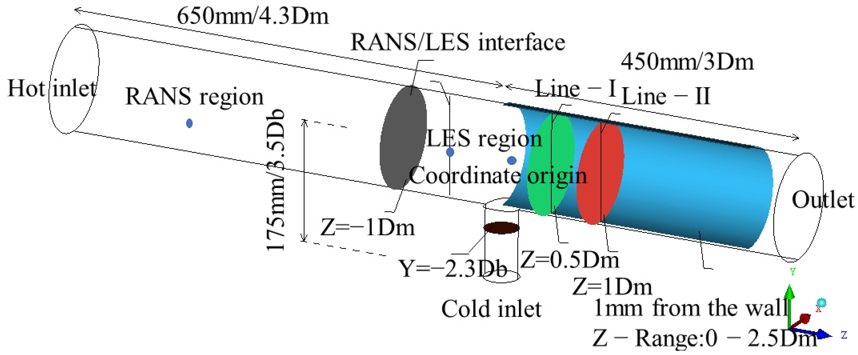
The k-omega SST model was used in the RANS portion to obtain the inlet velocity and turbulence quantities. The equations of the turbulence kinetic energy (k) and the specific dissipation rate (ω) for the SST k-ω model are as follows [28,29]:

$$\frac{\partial }{\partial x_i}\left(\rho k{u}_i\right)=\frac{\partial }{\partial x_j}\left[\left(\mu +{\mu }_t/{\sigma }_k\right)\partial k/\partial x_j\right]+G_k-Y_k$$

(11)

$$\frac{\partial }{\partial x_i}\left(\rho \omega u_i\right)=\frac{\partial }{\partial x_j}\left[\left(\mu +{\mu }_t/{\sigma }_{\omega }\right)\partial \omega /\partial x_j\right]+G_{\omega }-Y_{\omega }+D_{\omega }$$

(12)

The turbulent viscosity μ_t and terms such as G_k, Y_k, G_ω, Y_ω, D_ω are defined as:

$${\mu }_t=\frac{\rho k}{\omega }{\left[\text{max}\left(\frac{1}{{\alpha }^{*}},\frac{S{F}_2}{{\alpha }_1\omega }\right)\right]}^{-1}$$

(13)

$$\begin{array}{cc}{G}_k=\text{min}\left({\mu }_t{S}^2,10\rho {\beta }^{*}k\omega \right)& Y_k=\rho {\beta }^{*}k\omega \end{array}$$

(14)

$$\begin{array}{cc}{G}_{\omega }=\frac{{\alpha }_{\infty }}{{\alpha }^{*}}\left(\frac{{\alpha }_0+R{e}_t/2.95}{1+R{e}_t/2.95}\right)\rho S^2& Y_{\omega }=\rho {\beta }^{*}{\omega }^2\end{array}$$

(15)

$$D_{\omega }=2\left(1-F_1\right)\rho {\sigma }_{\omega ,2}\frac{1}{\omega }\frac{\partial k}{\partial x_j}\frac{\partial \omega }{\partial x_j}$$

(16)

2.3. Physical Model

The physical problem was that two streams of water at 48 °C with Pr = 3.7 and 33 °C with Pr = 5.1 flowed into the tee pipe from different inlets and mixed. The water experiments were conducted by Kamide et.al. In the experiment, hot and cold water entered the test section from a horizontal main pipe with a diameter of 150 mm (D_m) and a vertical branch pipe with a diameter of 50 mm (D_b), respectively. The main pipe of the test section had 18 D_m of the upstream length to the tee and it was 10 D_b in the branch pipe. In this study, the computational domain was established with entrance lengths of 650 mm (4.3 D_m) and 175 mm (3.5 D_b) from the tee with the same diameters as the test section. The downstream length was set as 450 mm (3 D_m) in the computational domain to cover the test results. A schematic diagram of the computational domain is shown in Figure 1. The cross-section at 1 D_m upstream of the tee of the main pipe was set as a RANS-LES interface, while the cross-sections at 0.5 D_m and 1 D_m downstream of the tee identified in Figure 1 were consistent with the test as monitor positions. In the main pipe, the upstream region divided by the RANS-LES interface was the RANS computational domain, while another one was the LES computational domain. Similarly, the cross-section at −2.3 D_b upstream of the tee of branch pipe was set as a RANS-LES interface. Besides, the coordinate origin was located at the intersection of pipe axes as shown in Figure 1.

2.4. Precursor Simulations

When the ELES simulations are carried out, unsteady fluctuations at the RANS-LES interface are required to be provided to the LES domain [19]. Therefore, precursor RANS simulations are conducted for the profiles of inlet turbulence quantities and the pre-estimation of mesh size in the central mixing zone, and the K-omega SST turbulence model is employed before carrying out the ELES. In the precursor RANS simulations, turbulent flows are conducted in pipes with a diameter of 1 D_m and 1 D_b, respectively. In order to obtain the fully developed inlet profiles, the pipe lengths are set as 18 D_m and 10 D_b, respectively, as the requirement stated in reference [19]. Through the precursor simulations, the profiles of inlet turbulence quantities can be obtained.

Precursor simulations of three cases with typical flow patterns are simulated in the pipes with the K-omega SST turbulence model. Details of the three cases are listed in

Table 1. Conditions of three typical cases.

Case	Average Velocity (m/s)		Momentum Ratio (MR)	Flow Pattern
	Main (Vm)	Branch (Vb)
W-ref	1.46	1	8.1	Wall jet
D-ref	0.46		0.8	Deflecting jet
I-ref	0.23		0.2	Impinging jet

. According to reference [5], the flow pattern can be predicted by the momentum ratio M_R: M_R < 0.35: impinging jet, 0.35 < M_R < 1.35: deflecting jet, M_R > 1.35: wall jet. Furthermore, the momentum ratio M_R is defined as Equation (17):

$$M_R=\frac{M_m}{M_b}=\frac{D_m{D}_b{\rho }_m{V}_m^2}{\raisebox{1ex}{$\pi $}\!\left/ \!\raisebox{-1ex}{$4$}\right.D_b^2{\rho }_b{V}_b^2}$$

(17)

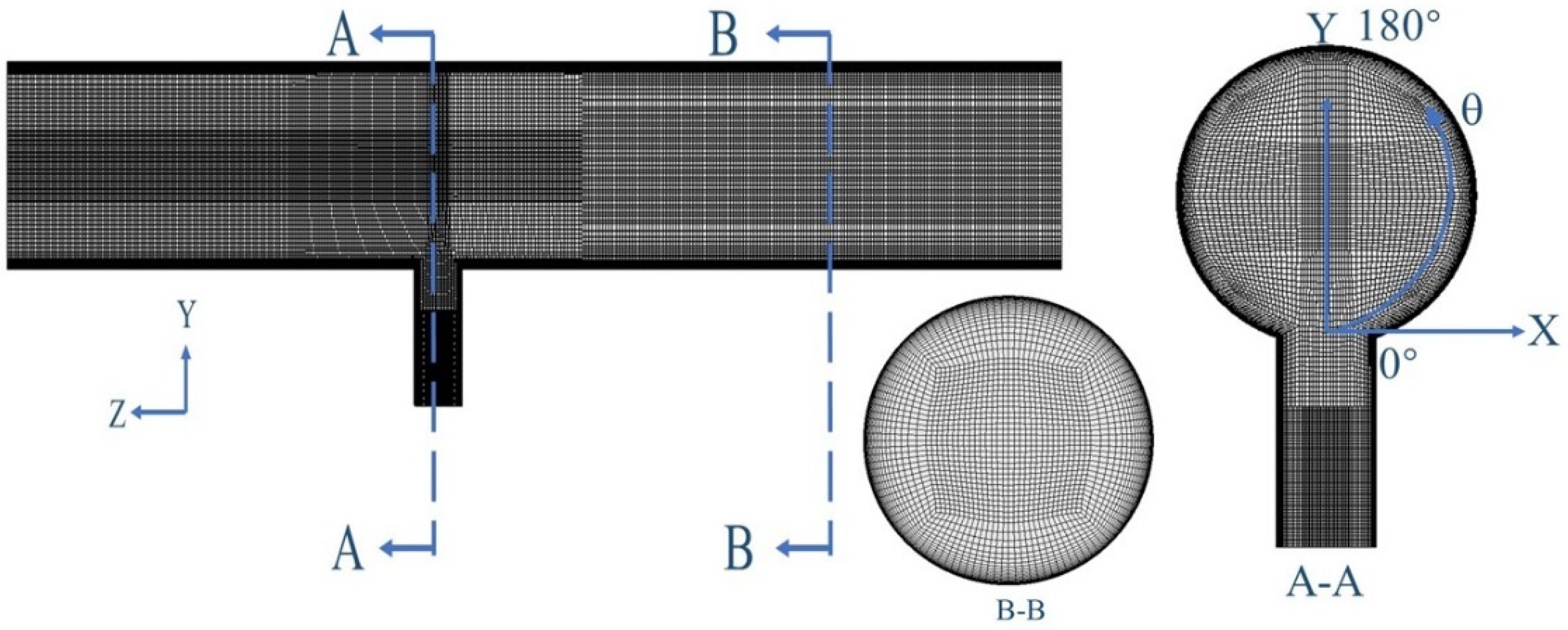
2.5. Meshing Requirement

2.5.1. Meshing Requirement near the Wall in the LES Portion

Quite a number of suggestions on the meshing requirements of LES have been given in the related literature. NJ Georgiadis et al. [30] gave the usual values of the grid spacing in three directions: Δz⁺ = 50–150, Δx⁺ = 15–40, and N_y = 60–80 beginning with Δy⁺ ≤ 1, where x, y, and z are the spanwise direction, the wall normal, and the streamwise, Δi⁺ is the non-dimensional grid spacing defined as Δi⁺ = u_τ Δi/v (i refers to x, y, and z), and N_y is the number of cells to cover the boundary layer in the wall-normal direction. This is a typical requirement for classic wall-resolved LES, and the values of the actual grid spacing (Δi) would be Re-dependent in practice.

Meanwhile, in applications with a wall-modeled LES formulation, the requirement can be relaxed. In the wall-normal direction, although a coarser Δy⁺ value such as Δy⁺ ≈ 20 [31] can be tolerable, a near-wall resolution of Δy⁺ = 1 was taken in the current work and the number of cells across the boundary layer was set as N_y = 60 as recommended by ANSYS. A typical wall-normal grid spacing Δy of the main pipe was set as 0.02 mm to ensure the near-wall resolution in the current work had a Re number of approximately 3.9 × 10⁵. In the other two directions, the grid spacing Δx ≈ Δz ≈ (0.05–0.1)δ was adopted in the current work as recommended by ANSYS, where δ (mm) is the per boundary layer thickness. The Δx/Δz of the main pipe was fixed at 2.25 mm/3.75 mm in the current work, and (Δx⁺, Δz⁺) ≈ (113, 188) in wall units with a Re number of approximately 3.9 × 10⁵.

2.5.2. Meshing Requirement in the Mixing Zone Downstream in the LES Portion

To meet the mesh resolution of the separating shear layer in the mixing zone downstream, Addad et al. [32] recommended a minimal LES mesh resolution with which the mesh size Δ was taken as max (λ_R, L_t^R/10), where the Taylor microscale λ_R and the turbulent energy length L_t^R were both obtained from RANS estimations, as seen in Equations (18) and (19).

$${\lambda }_R=\sqrt{10k\nu /\epsilon }$$

(18)

$$L_t^R=\frac{k^{\raisebox{1ex}{$3$}\!\left/ \!\raisebox{-1ex}{$2$}\right.}}{\epsilon }=\frac{k^{\raisebox{1ex}{$1$}\!\left/ \!\raisebox{-1ex}{$2$}\right.}}{0.09\omega }$$

(19)

Kuczaj et al. [33] concluded that the mesh size of Δ ≈ λ/3, where λ was the Taylor microscale obtained from a posteriori LES analysis, can give sufficiently accurate results, and the value of λ/3 was found to be equivalent to the RANS Taylor microscale λ_R. X Fang et al. [31] recommended a mesh size of Δ/η_R < (50–100) for LES mixing layers, where the Kolmogorov scale η_R can be calculated as Equation (20):

$${\eta }_R=L_t^R{(\raisebox{1ex}{$k^2$}\!\left/ \!\raisebox{-1ex}{$\epsilon \nu $}\right.)}^{\raisebox{1ex}{$-3$}\!\left/ \!\raisebox{-1ex}{$4$}\right.}$$

(20)

Here, when non-equilateral cells are used, the mesh scale Δ refers to max (Δx, Δy, Δz); in addition, k, ε, and ω are the turbulent kinetic energy, the turbulent dissipation energy, and the specific dissipation rate, respectively. Eventually, the mesh scale of the free shear portion was set as Equation (21):

$$\Delta =\mathit{\text{min }}({\lambda }_R,L_t^R/10,50{\eta }_R)$$

(21)

As precursor RANS simulations were performed, a typical mesh size was obtained by the above estimator, that is Δ = 2.5 mm in the free shear portion. Then, hexahedral structure grid elements were constructed in the current work.

2.5.3. Meshing Requirement in the RANS Portion

After the details of meshing requirements in the LES portion are emphasized, the resolution requirements in the RANS portion should be determined. It is recommended that the wall boundary layer should be covered with (20–30) cells with y⁺ ~ 1, and the minimum resolution across free shear flows can follow Equation (22).

$${\Delta }_{\max }\le 0.05D$$

(22)

Therefore, we set Δ = 7.5 mm in the RANS portion as the coarser mesh can be accepted in this domain.

Finally, a typical grid structure with a total of approximately 4 million elements is shown in Figure 2. The A–A cross-section is in the LES portion and the B–B cross-section is in the RANS portion. It can be seen that the mesh in the RANS portion is much coarser than that in the LES portion, which will reduce the number of grids in the whole computational domain, as well as the computation cost.

In order to assess the grid independence, four types of grids shown in Figure 3 were made according to the above criteria. They had approximately 0.5, 1.6, 4.0, and 6.4 million cells, and the information is listed in

Table 2. Information for grid independence.

Case	Treatment near the Wall	Treatment in the Free Shear Layer	Criteria
Case-A	Ny = 30, Δy1 = 0.02, y+ ~ 1	Δ < 5	More relaxed requirements put forward by NJ Georgiadis et al. [28] and Equation (21)
Case-B	Ny = 60, Δy1 = 1, y+ ~ 50	Δ < 2.5	Strict requirements put forward by NJ Georgiadis et al. [28] and Equation (21)
Case-C	Ny = 60, Δy1 = 0.02, y+ ~ 1	Δ < 2.5	More relaxed requirements put forward by NJ Georgiadis et al. [28] and Equation (21)
Case-D	Ny = 80, Δy1 = 0.02, y+ ~ 1	Δ < 1.5	Strict requirements put forward by NJ Georgiadis et al. [28] and Equation (21)

(cases are defined as Case-A, Case-B, Case-C, and Case-D in ascending order of the grid’s number). The cell thickness of the first layer from the pipe’s inner surface is marked as Δy₁. Additionally, the grid independence is covered in more detail in Section 3.1.

2.6. Boundary Conditions and Numerical Setting

The vortex method [34] was adopted to generate turbulent fluctuations at RANS-LES interfaces in the simulations. The number of vortices was set to be large enough to affect all spots on the face zone. For the inlet boundaries, the profiles of velocity and turbulence quantities obtained from precursor RANS simulations were specified. For the solid boundaries, the pipe walls were set under non-slip and adiabatic conditions.

As recommended in reference [19], the time steps should be chosen to achieve a Courant number of CFL~1 in the LES portion. Therefore, the time step was set as 0.001 s in our simulations, which leads to CFL~1 in the central mixing zone. The mass conservation was most concerned in the process of convergence, and the mass residuals decreased by more than 10 orders of magnitude each time step with 20 inner iteration loops. Other numerical settings and related information in the current simulations are listed in

Table 3. A summary of the current numerical simulation.

Numerical Settings
Spatial discretization	Momentum	Bounded central differencing in LES; 2nd order upwind in RANS
	K & Ω	2nd order upwind in RANS
	Gradients	1st order upwind
	Pressure	2nd order upwind
Time Discretization	Transient formulation	Bounded second order implicit
	Time advancement	Iterative time advancement with SIMPLEC scheme
	Time step interval	0.001 (s)
	Iteration every 1 time-step	20 iterations
Models	RANS portion	K-omega SST
	LES portion	WMLES
Precursor simulations	RANS domain	K-omega SST

.

As for the physical properties of the water, the density, specific heat capacity, and coefficient of thermal conductivity change slightly with the temperature, hence, the three physical properties are treated as constant. However, the dynamic viscosity changes a great deal with the temperature and it seems that the dynamic viscosity is approximately linear with a temperature between 33 °C and 48 °C; therefore, a UDF was constructed, and the detailed code can be seen in Appendix A.

3. Simulations with the Numerical Method ELES

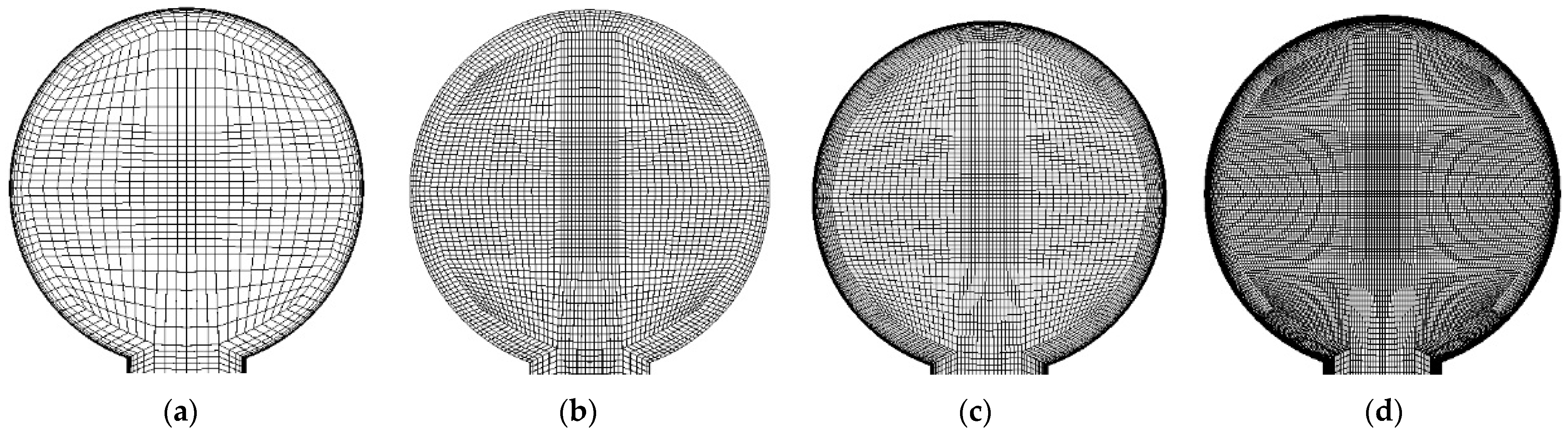
3.1. Meshing and Independence Validations for Grid

The different mesh requirements used in simulation may influence the computational accuracy and the computational time. Therefore, a grid independence check was performed before the numerical computation to establish an appropriate grid structure in order to maintain a balance between computational accuracy and time. Four cases using the different mesh requirements listed in Table 2 were selected for comparison under the same computational conditions.

Additionally, two statistical variables, which were mean axial velocity V_Z and axial velocity fluctuation intensity at position Z = −0.53 D_m in the W-ref case, were taken as a comparison. Both the mean velocity and the intensity were normalized by the bulk velocity in the main pipe, V_m. Definitions are as below:

$${\overline{V}}_z^{*}=\frac{{\overline{V}}_z}{V_m}$$

(23)

$$V_{z-sd}^{*}=\frac{1}{V_m}\sqrt{\frac{{\displaystyle {\sum }_i{(V_z^i-{\overline{V}}_z)}^2}}{N}}$$

(24)

where N is the total number of sampling data and V_zⁱ is an instantaneous value at a certain position along the vertical line.

Considering that the frequency of the particle image velocimetry (PIV) used in reference [5] was 15 Hz (0.066 s) and approximately 17 s for the measurement, just for comparison, the sampling interval was set as 0.066 s (66 time-steps) and a period of approximately 10 s was taken for statistics after calculation convergence in the current work.

The simulation results of four grids are shown in Figure 4. It shows that the results reproduce the tendency of the distribution pretty well. At −0.53 D_m upstream of the tee, there is no big difference between the mean axial velocity among the grids. Although the results of the four cases vary to some degree, the calculated mean axial velocity is in good agreement with the measured data. However, the results of the axial velocity fluctuation intensity in Case-C and Case-D show better than that of Case-A and Case-B. Case-A underestimated the experimental data, while Case-B performed worse predictions near the wall than others. Considering the computational cost, Case-C seems the best choice among the four grids since it not only has high enough accuracy but also saves computational resources. Therefore, the grid structure of Case-C was selected in the present research.

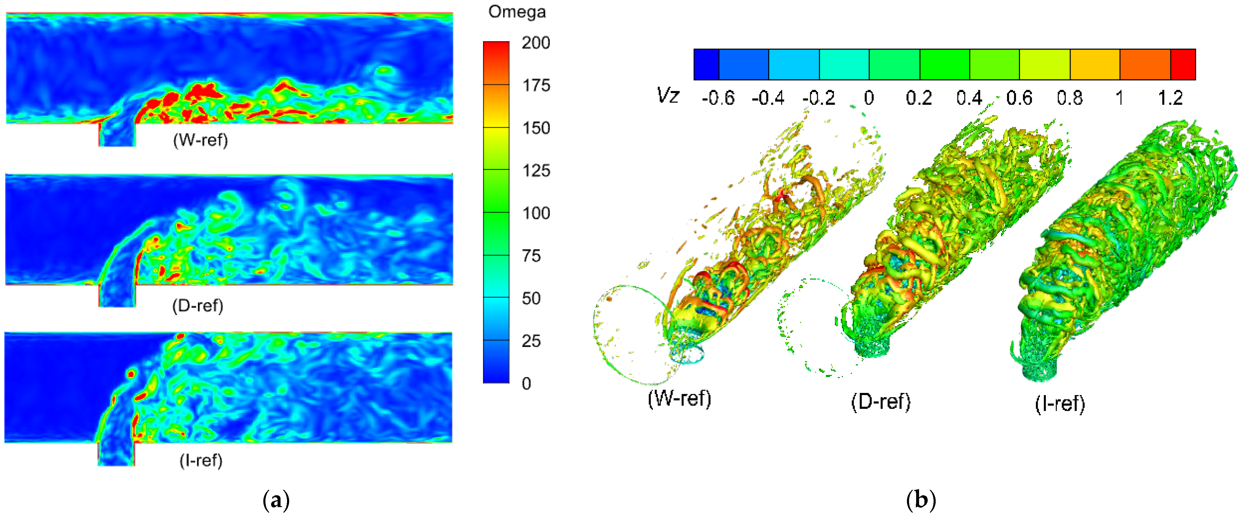
3.2. Turbulence Generation and Structure

Three cases with typical flow patterns listed in Table 1 were simulated with ELES. Before processing the validation of the ELES model, some work needs to be completed such as checking the turbulence generation and structure.

By vorticity post-processing, Figure 5a shows that the resolved turbulences were well-generated from the upstream interfaces in the three reference cases. Here, the vorticity (omega) has projections in the Cartesian coordinate system as seen in Equation (25):

$${\mathrm{\Omega }}_x=\frac{\partial V_z}{\partial y}-\frac{\partial V_y}{\partial z},{\mathrm{\Omega }}_y=\frac{\partial V_x}{\partial z}-\frac{\partial V_z}{\partial x},{\mathrm{\Omega }}_z=\frac{\partial V_y}{\partial x}-\frac{\partial V_x}{\partial y}$$

(25)

Additionally, the turbulence structures in the current ELES simulations need to be checked. Figure 5b shows iso-surfaces of the Q-criterion colored with V_z in three cases. Turbulence structures are depicted to be well-developed and show no damping or disruption downstream. The definition of Q is defined as Equation (26):

$$Q=\frac{1}{2}\left({\mathrm{\Omega }}^2-S^2\right)$$

(26)

where S is the strain rate and Ω is the vorticity, and both are absolute values. The iso-surfaces of the Q-criterion shown in Figure 5b are equal to 200 [s⁻²]. The above analysis reveals that the current ELES simulations provide high resolution on turbulence structures in LES zones with the vortex method adopted at the upstream interface.

3.3. Validation of the Numerical Method ELES

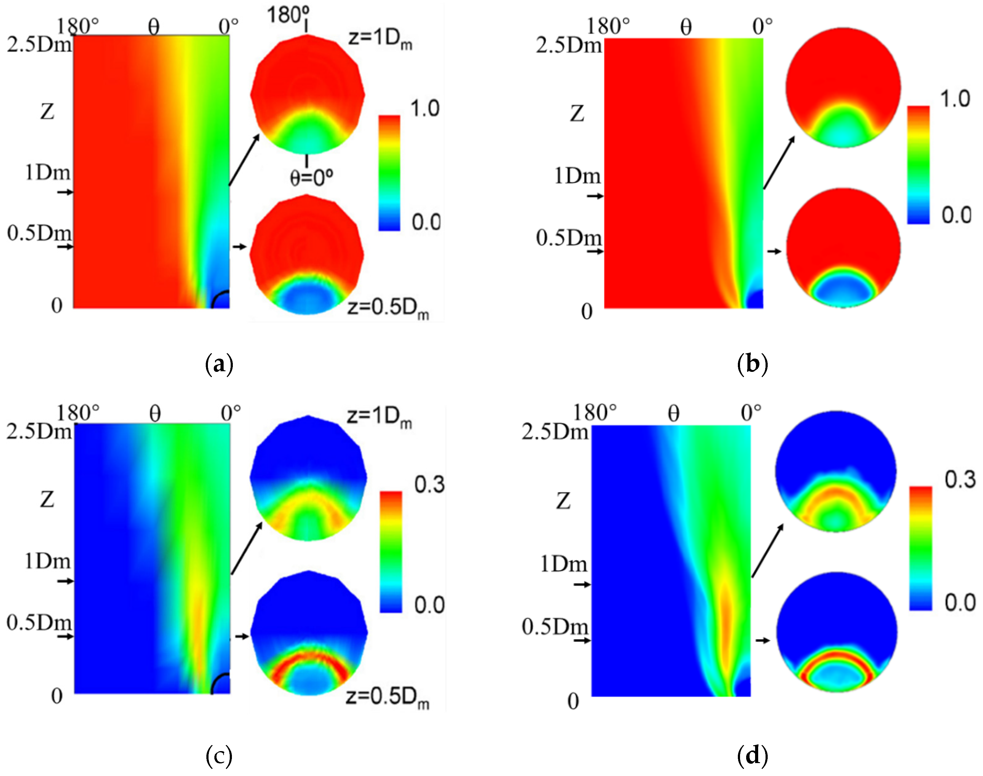
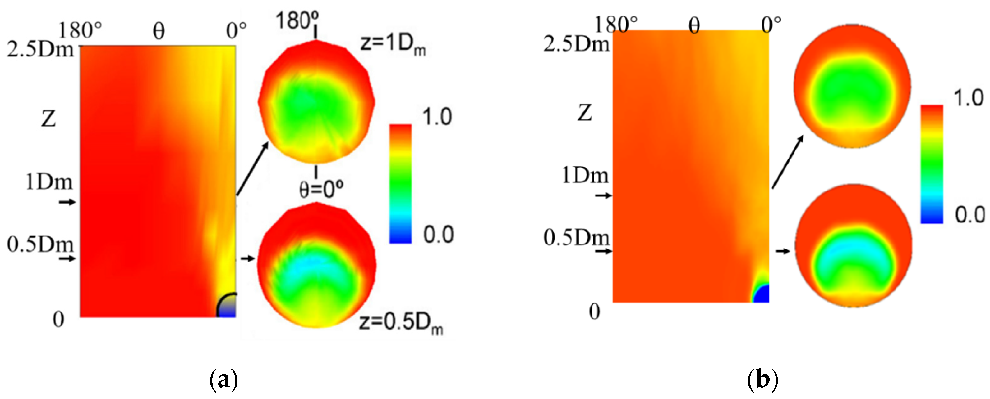
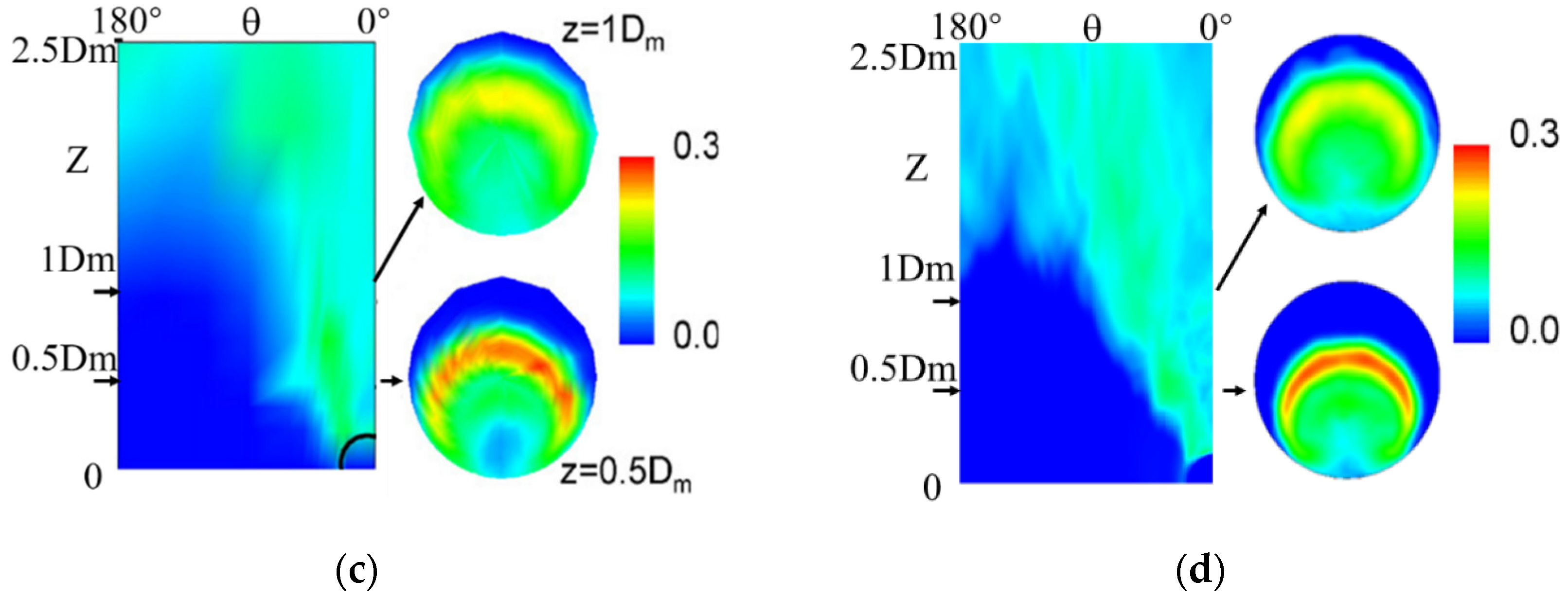
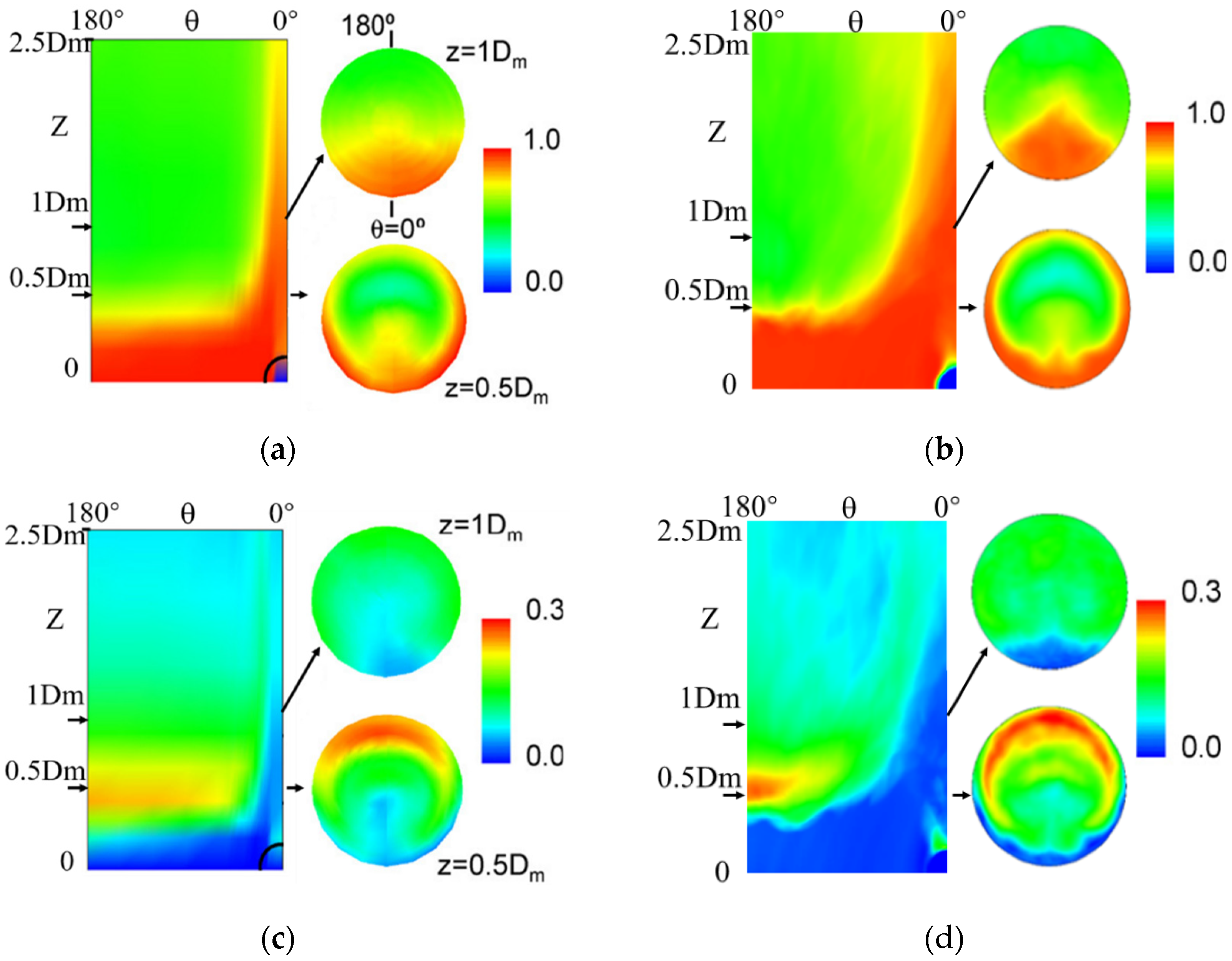
3.3.1. The Contours of Temperature and Velocity Distributions Downstream

The distributions of temperature and fluctuation intensity on a half-cylindrical surface 1 mm apart from the main pipe wall and two cross-sections downstream (as shown in Figure 1) were obtained by simulation. Figure 6, Figure 7 and Figure 8 show comparisons of these statistical results and the experimental ones. The left sides of Figure 6, Figure 7 and Figure 8 are the LES results of Kamde et al. [5]. using the AQUA code, which is an in-house thermal hydraulic simulation code [35]. The right sides are the ELES simulation results using FLUENT 17.0.

The data displayed in Figure 6, Figure 7 and Figure 8 were normalized with the temperature difference as seen in Equations (21) and (22):

$${\overline{T}}^{*}=\frac{\overline{T}-T_b}{T_m-T_b}$$

(27)

$$T_{sd}^{*}=\frac{1}{T_m-T_b}\sqrt{\frac{{\displaystyle {\sum }_i{(T_i-\overline{T})}^2}}{N}}$$

(28)

Here, T_b is the branch temperature and (T_m − T_b) is the temperature difference fixed at 15 °C, T is the time-averaged temperature at a certain position on a surface, and N is the total number of sampling data. Considering that the sampling frequency was 100 Hz and the measurement time period was 480 s in reference [5], just for comparison, the sampling interval was set as 0.01 s (10 time-steps), and a period of approximately 100 s was taken for statistics after calculation convergence in the current work.

It can be found that the numerical values and distributions in Figure 6, Figure 7 and Figure 8 show good agreement. It can be clearly seen in Figure 6, Figure 7 and Figure 8 that the thermal stripping phenomenon appears and the high fluctuation intensity occurs around the cold fluid in contact with the hot. In the W-ref case, the high-intensity region touched the pipe wall to form a half-circle big-value area at each radial cross-section, while in the deflecting jet case, the high-intensity region was separate from the pipe wall because the cold fluid from the branch pipe flowed into the central part of the main pipe. On the other hand, the cold jet from the branch pipe reached the opposite side pipe wall in the impinging jet case, and the high-intensity region then appeared in the upper half of the main pipe and decreased rapidly in the axial direction.

As can be seen from the distribution results in radial cross-sections, along the main flow direction downstream in all three cases, the temperature range narrowed and the maximum fluctuation intensity decreased, which suggested gradually sufficient mixing was obtained with the flow.

The main difference between the ELES results and the LES ones conducted by Kamide et al. [5] shown in Figure 6, Figure 7 and Figure 8 is that the temperature distributions near the wall of ELES are much clearer than that of LES, which indicates that ELES is better able to capture temperature fluctuations near the wall.

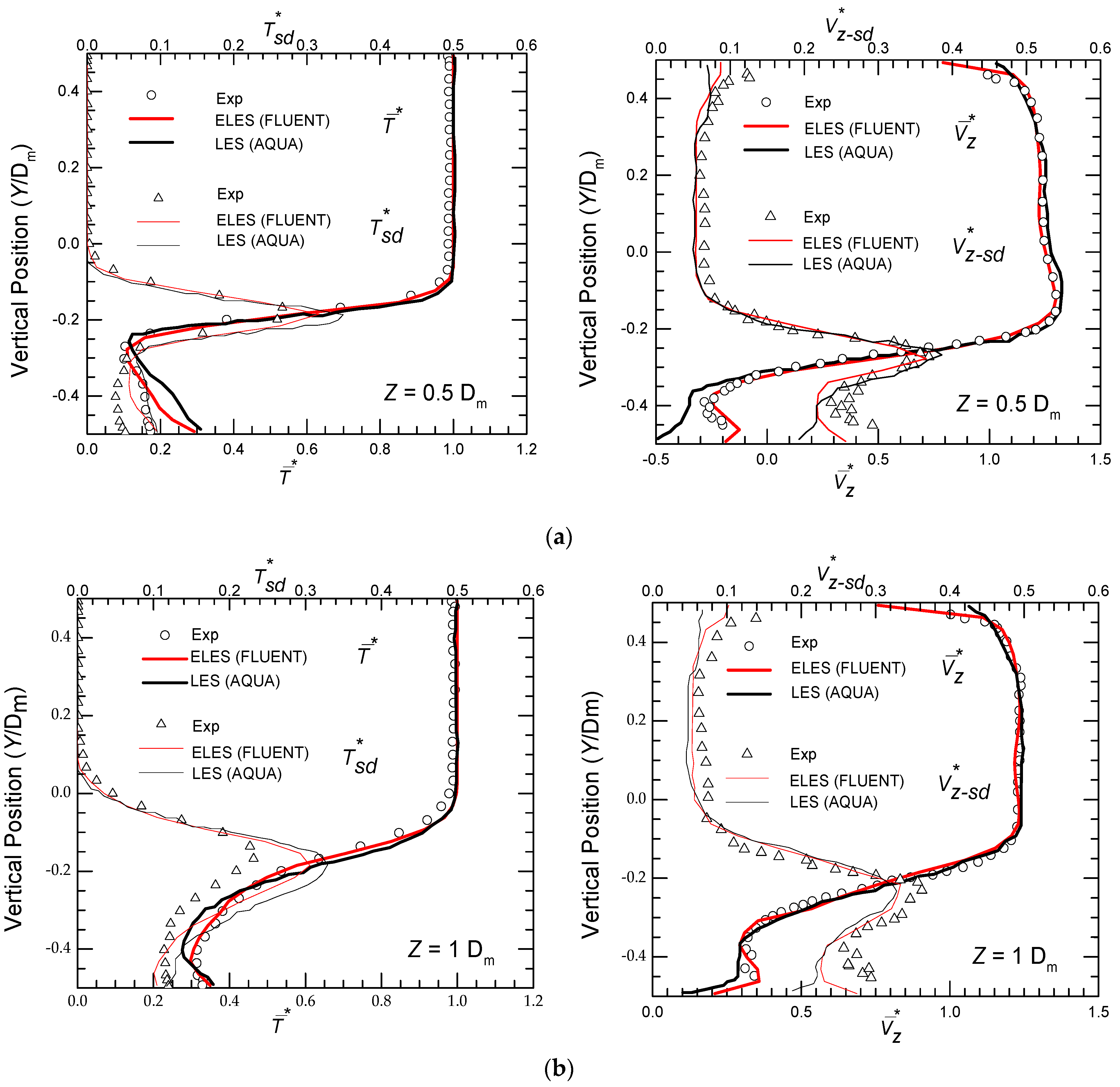
3.3.2. Temperature and Velocity Distributions Downstream along Vertical Lines

Spatial distributions of the axial velocity component V_z, the temperature, and their fluctuation intensities along the vertical lines at position Z = 0.5 and 1 D_m in the W-ref case were compared and are shown in Figure 9 (vertical lines named ‘line-I’ and ‘line-II’ are shown in Figure 1).

The calculated distributions were in good agreement with those in the experiment. The fluctuation intensities were well-simulated to obtain peak values at positions where the physical quantity had a sudden change along the vertical direction. The distribution trends of temperature were similar to that of the axial velocity component, and both their obvious features appeared at the position around Y = −0.2 D_m. The velocity fluctuation intensities were slightly underestimated within ELES simulations, and it was considered that the fluctuations were actually enhanced in the experiments due to the dense arrangement of quite a number of thermocouples.

In addition, the peak values of the temperature fluctuation intensity were overestimated in ELES analyses, especially at the downstream position Z = 1 D_m (the same in AQUA analyses performed by Kamide et al. [5]), which indicated that it became thermal mixing in the actual flow likely because of the enhancement of the velocity field disturbance downstream during the experiment. In addition, it obtained more appropriate results near the wall with ELES, especially for the capture of the velocity fluctuation intensity, than that in AQUA analyses performed by Kamide et al. [5].

4. Results and Discussion

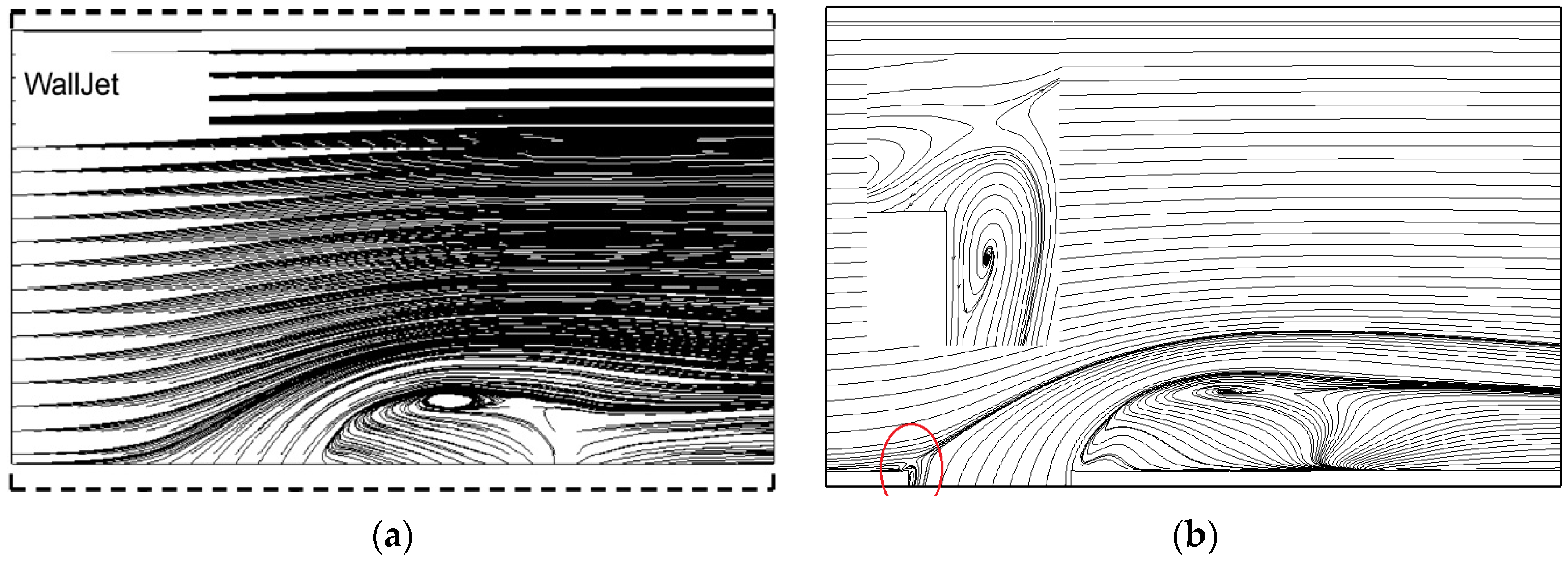
4.1. The Phenomena of Backflow

As a comparison to the LES results conducted by Kamide et al. [5] shown in Figure 10a, mean axial and vertical velocities were used to depict the time-averaged streamlines in the y–z plane in the W-ref case, and the characteristics of the jet bending and eddies’ formation obtained with ELES are shown in Figure 10b, which show good agreement. On the other hand, due to the prediction ability near the wall of ELES, it was found that backflow happened near the wall around the tee region, which had not been mentioned in the LES results conducted by Kamde et al. [5]. It was noteworthy that these phenomena were not special cases at certain moments as they were mean results. It can be seen as a vortex generated by backflow, which drives the mixing of hot and cold flows.

In order to study the influence of temperature fluctuation caused by the backflow near the wall around the tee region, a y–z plane of W-ref case at X = 0 was taken to form the contour of temperature fluctuation intensity, the result of which is shown in Figure 11. Figure 11a shows the overview of temperature fluctuations around the right-angle structure upstream of the tee, and temperature fluctuations in the region approximately 1 mm away from the wall are shown in Figure 11b. It can be found from Figure 11 that the temperature fluctuation intensity is close to 0.3, which is almost the same downstream of the pipe shown in Figure 6, Figure 7 and Figure 8. Obviously, the right-angle structure upstream where the welding exists is exposed to temperature fluctuations, which makes the thermal stress-sensitive area more prone to fatigue failure. Therefore, the phenomena of the backflow in the tee region are vital to the study of thermal fatigue and need more attention.

In the following, more detailed quantitative analyses are further carried out to form a comprehensive understanding of the backflow in thermal mixing and the relationship between fatigue and backflow in the tee.

4.2. Characteristics of Backflow in the Tee

Backflow is widespread in non-isothermal mixing in the tee, and these phenomena are closely related to the momentum ratio of the main to branch flow. Therefore, to fully study these phenomena and understand the mechanism of the backflow in the tee, 12 groups of simulations with different momentum ratios were carried out and the flow field characteristics were analyzed. Detailed information on the simulations is listed in

Table 4. Groups of simulations with different momentum ratios with average branch velocity V_b = 1 m/s.

Case	Average Main Velocity (Vm) (m/s)	Momentum Ratio (MR)	Flow Pattern
Case1	0.11	0.05	Impinging jet
Case2	0.16	0.1	Impinging jet
Case3	0.20	0.15	Impinging jet
Case4	0.23	0.2	Impinging jet
Case5	0.46	0.8	Deflecting jet
Case6	1.46	8.1	Wall jet
Case7	1.74	11.5	Wall jet
Case8	1.76	11.8	Wall jet
Case9	1.78	12	Wall jet
Case10	1.85	13	Wall jet
Case11	1.95	14.5	Wall jet
Case12	2.9	32	Wall jet

.

The streamline diagrams of the three impinging jet cases were compared and the results are shown in Figure 12a–c. The streamline diagrams were drawn in the y–z plane at X = 0. Figure 12a–c shows that when the flow rate of branch flow is high enough, the upper fluid of the main flow is squeezed into a vortex and the phenomena of the backflow appear near the opposite sidewall. The higher the flow rate, the larger the eddy and the more obvious the phenomena of the backflow. When M_R ≤ 0.1, the backflow with large eddies occurs near the opposite sidewall upstream. The results are similar to the experiments conducted by several researchers, e.g., Mei-Shiue Chen et al. [36], C.H. Lin et al. [37], G.Y. Chuang and Y.M. Ferng [38,39], and Wu et al. [40] In their research, the phenomena of the backflow occurred when M_R ≤ 0.05, M_R ≤ 0.062, M_R ≤ 0.06, and M_R ≤ 0.05, respectively. The difference may be the limit of observation methods in the experiment regarding the inadequate sensitivity of temperature sensors.

As the velocity of the branch flow decreases, so does the vortex, and when M_R = 0.2, the phenomena of the backflow that appear near the opposite sidewall almost disappeared and gradually transitioned to the place of the right-angle structure upstream of the main flow, as shown in Figure 12d. As the velocity of the branch flow decreases and that of the main flow increases, the vortex formed by backflow becomes larger at the right-angle structure upstream of the branch flow, as shown in Figure 12e–f. Compared with the size of the eddies near the opposite sidewall upstream when M_R ≤ 0.1, the eddies shown in Figure 12d–f are relatively small, which may be the main reason that researchers have rarely observed the phenomena.

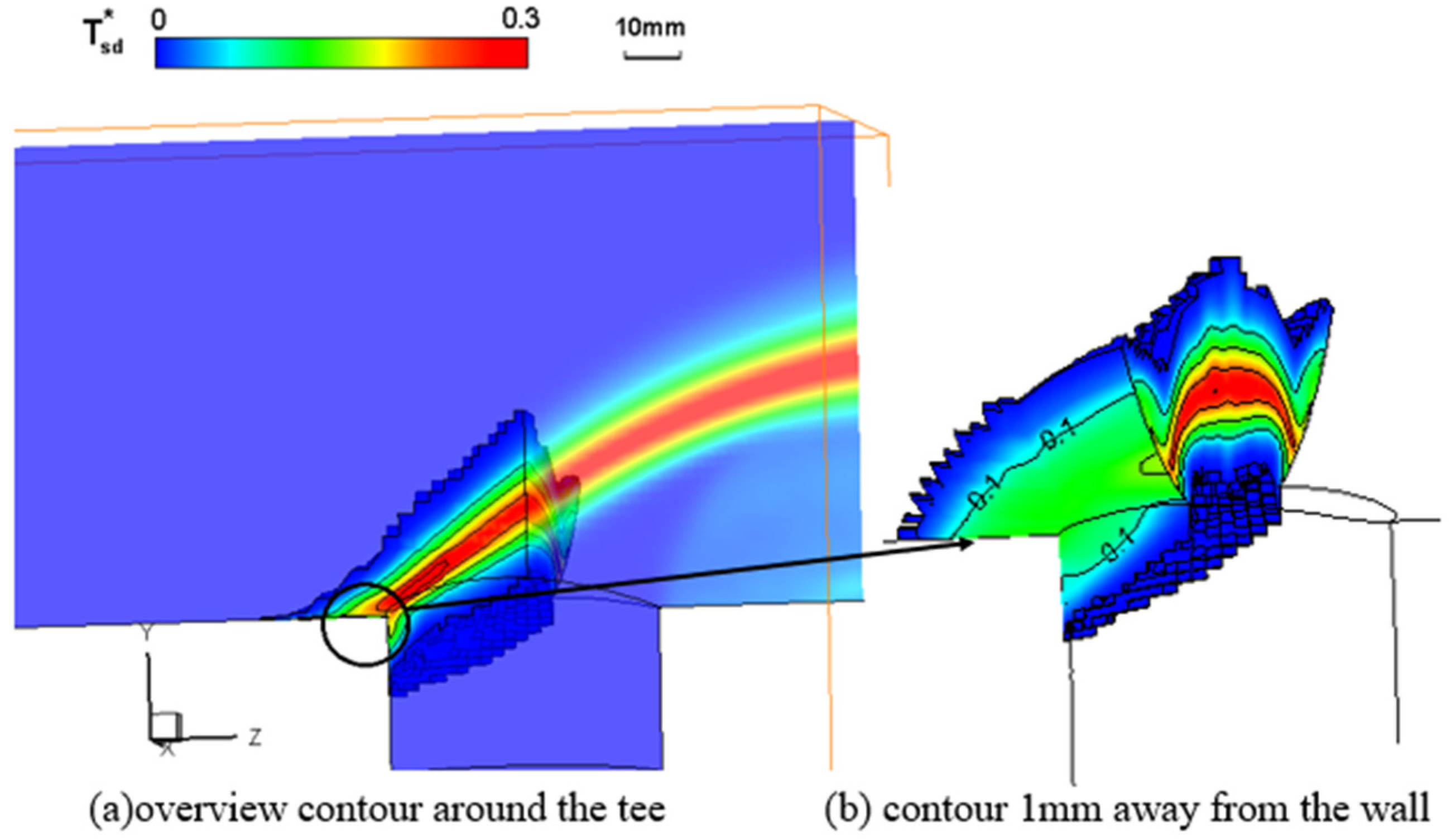
4.3. Temperature Characteristics near the Wall Where Backflow Appears

It can be found from the above research that different flow patterns with different momentum ratios have different characteristics of the backflow. In order to study the temperature distributions related to the backflow, detailed studies have been carried out under typical conditions in each flow pattern. From Figure 12, three typical cases with the most obvious characteristics of the backflow were chosen as the representative of each flow pattern, which were Case1 with M_R = 0.05, Case7 with M_R = 0.8, and Case12 with M_R = 32. Additionally, the temperature was recorded at every time step with a sampling frequency of 1000 Hz for a duration of 74.8 s.

Axial distributions of the temperature fluctuation intensity of the above cases along corresponding lines are depicted in Figure 13. The corresponding lines of the three cases described in Figure 13 are 1 mm away from the wall. From the distribution of temperature fluctuation along line1 in Figure 13, we can see that the axial range affected by thermal striping is very wide, and it also seems that there exists more than one peak, with a maximum of approximately at Z = −0.5 D_m upstream, which indicates that the thermal mixing caused by the backflow is complex. In addition, the temperature fluctuation intensity at Z = −0.5 D_m shown in Figure 13 is close to that of 0.5 D_m downstream plotted in Figure 6, Figure 7 and Figure 8. In order to further study the mixing behavior, two contours were plotted at the cross-sections of Z = −0.5 and −0.2 D_m upstream as shown in Figure 14a,b. As we can see from Figure 14a,b, thermal striping appears near the opposite wall of the branch pipe, and the temperature fluctuation intensities in some locations are relatively high such as points near the wall at 105° and 180° of the cross-section at Z = −0.2 D_m and the point near the wall at 180° of the cross-section at Z = −0.5 D_m.

From the distribution of temperature fluctuation along line2 in Figure 13, we can see that the temperature fluctuation intensity is relatively low and the axial range affected by thermal striping is narrow, which indicates that the thermal mixing is not fully developed although there exists a relatively larger eddy as shown in Figure 12d. The main reason for this phenomenon may be that the momentums of the main and branch flows are similar as M_R = 0.8. When each flow blocks the other one in the tee with M_R ~ 1, there is not enough power for one to penetrate upstream of the other one. A contour plotted at the cross-section of Z = −0.18 D_m upstream as shown in Figure 14c reveals the above view. Therefore, the depth of penetration of one to another is dependent on the momentum ratio.

From the distribution of temperature fluctuation along line3 in Figure 13, we can see that although the axial range affected by the thermal striping is narrow, the temperature fluctuation intensity is relatively higher compared with that of Case1 and Case7. With the penetration depth, the temperature fluctuation intensity tends to increase and then decrease, and a peak of approximately 0.32 appears at the location of Y = −1.55 D_b. Figure 14d shows the temperature distributions at Y = −1.55 D_b. It can be seen that the phenomenon of thermal striping is very significant, and the radial range affected by the thermal striping is wide as it is from −90° to 90°. Meanwhile, the fluctuation peak appears at θ = 45° in Figure 14d.

In order to analyze the frequency characteristics (PSD), the FFT method was applied to the data extracted over a period of 74.8 s and presented in Figure 15. The prominent frequency components were observed in all analyses in Figure 15. At Z = −0.5 D_m, θ = 180° of Case 1 in Figure 15, frequency peaks appeared at 0.5 Hz, 0.8 Hz, 1.2 Hz, 1.97 Hz, 2.53 Hz, 3.3 Hz, 6.31 Hz, etc.; at Z = −0.2 D_m, θ = 105°, frequency peaks appeared at 0.47 Hz, 1.26 Hz, 2.63 Hz, 5.68 Hz, etc.; while at Z = −0.2 D_m, θ = 180°, frequency peaks appeared at 0.48 Hz, 1.27 Hz, 2.60 Hz, 5.78 Hz, etc. Although the peaks did not exactly match, they were similar in the three locations. Besides, it is generally known that the frequency approaching 6 Hz in Figure 15 corresponds to the frequency of the Karman vortex street. In addition, the characteristic frequency was not very significant, at approximately 6 Hz downstream shown in references [5,10], but long-period temperature fluctuations of frequencies lower than 6 Hz upstream from the tee were found, which had also been observed by Utanohara et al. [10] downstream. As described in Smith et al. [41] and Thomas [42], long-period temperature fluctuations of a low frequency (0.1–10 Hz) would cause the most harmful thermal loads. Hence, the conditions may require more attention.

At Z = −0.18 D_m, θ = 0° of Case 7 in Figure 15, frequency peaks appeared at 0.49 Hz, 0.89 Hz, 1.47 Hz, 2.75 Hz, 6.0 Hz, etc., while at Y = −1.5 D_b, θ = 45°of Case 12, frequency peaks appeared at 0.95 Hz, 1.55 Hz, 3.2 Hz, 5.76 Hz, etc. The characteristic frequency of approximately 6 Hz in the two cases seems more obvious than that in case1, which is because the phenomena that occurred at the points in case7 and case12 are more similar to the phenomena of the Karman vortex street. Moreover, a long-period temperature fluctuation of a frequency lower than 6 Hz upstream (e.g., approximately 0.5 Hz, 1.2 Hz, 3.0 Hz, etc.) from the tee was observed, too. This may be related to the periodic variation of the backflow around the attached wall. The long-period temperature fluctuation of a frequency lower than 6 Hz downstream from the T-junction was also seen in the experimental investigation by Miyoshi et al. [43] and the numerical study by Utanohara et al. [10]. However, it requires further study to validate the long-period fluctuation of a frequency lower than 6 Hz upstream through more experiments.

In sum, by analyzing the temperature distribution of three different flow patterns with different M_R values, three more regions are found to be prone to thermal fatigue at the intersection of the tee upstream. The effects of fatigue are different in the three regions. It seems that the impinging jet with a smaller M_R and the wall jet with a larger M_R have a greater possibility of fatigue crack on the wall around the intersection, while the effect of fatigue caused by the deflecting jet on the wall seems less significant.

5. Conclusions

In this paper, the mixing flow of non-isothermal fluids in tee pipes upstream is numerically studied in detail. Firstly, three typical flow patterns of thermal mixing in tee pipes (wall jet with M_R = 8.1, deflecting jet with M_R = 0.8, and impinging jet with M_R = 0.2) were simulated using the ELES method, and the results have been compared with the experimental data in reference [5] to prove the validity of the model. Secondly, the flow characteristics of the backflow upstream with different momentum ratios were studied by carrying out 12 groups of simulations using ELES, as well as the temperature characteristics near the wall where the backflow appears. Moreover, in order to evaluate the thermal fatigue, the frequency analysis at specified points near the wall of three typical flow patterns was estimated. The conclusions are summarized below:

(1)

ELES is a valid tee pipe numerical turbulent-solving method and aptly predicts the flow patterns of non-isothermal mixing in tee pipes.

(2)

The characteristics of the backflow in the tee are obviously different with different momentum ratios M_R. The relatively general rules are that the eddies caused by the backflow appear near the opposite sidewall of the branch pipe for cases of the impinging jet when M_R ≤ 0.1, the eddies appear near the wall at the right-angle structure upstream of the main pipe for cases of the deflecting jet when M_R ~ 0.8, while the eddies appear near the wall at the right-angle structure upstream of the branch pipe for cases of the wall jet when M_R ≥ 11.5. In addition, the size of the eddies caused by the backflow is dependent on M_R.

(3)

The characteristics of temperature distribution and the frequency of temperature fluctuations are different under different backflow patterns with different momentum ratios M_R. Besides the pipe wall downstream, three more regions are found to be prone to thermal fatigue at the intersection of the tee upstream. The effects of fatigue are different in the three regions. It seems that an impinging jet with smaller M_R and a wall jet with larger M_R have a greater possibility of fatigue cracks on the wall around the intersection, while the effect of fatigue caused by the deflecting jet on the wall seems less significant.

(4)

Long-period temperature fluctuations of frequencies lower than 6 Hz upstream (e.g., approximately 0.5 Hz, 1.2 Hz, 3.0 Hz, etc.) from the tee were observed, and they may be related to the periodic variation of the backflow around the attached wall. Besides, this requires further study to validate the long-period fluctuation of a frequency lower than 3 Hz upstream through further experiments.

References

1. Blondet, E.; Faidy, C. High Cycle Thermal Fatigue in French PWR. In Proceedings of the ASME 10th International Conference on Nuclear Engineering, Arlington, VA, USA, 14–18 April 2002; Volume 1, pp. 429–436. [Google Scholar] [CrossRef]
2. Gelineau, O.; Escaravage, C.; Simoneau, J.P.; Faidy, C. High cycle thermal fatigue: Experience and state of the art in French LMFRs. In Proceedings of the SMiRT16, Washington, DC, USA, 12–17 August 2001. Paper ID 1311. [Google Scholar]
3. Simoneau, J.P.; Noe, H.; Menant, B. Large eddy simulation of mixing between hot and cold sodium flows—Comparison with experiments. In Proceedings of the 7th International Meeting on Nuclear Reactor Thermal Hydraulics (NURETH-7), Saratoga, CA, USA, 10–15 September 1995; pp. 1324–1332. [Google Scholar]
4. Wakamatsu, M.; Hirayama, H.; Kimura, K.; Ogura, K.; Shiina, K.; Tanimoto, K.; Mizutani, J.; Minami, Y.; Moriya, S.; Madarame, H. Study on high-cycle fatigue evaluation for thermal striping in mixing tees with hot and cold water (1). In Proceedings of the 11th International Conference on Nuclear Engineering, Tokyo, Japan, 20–23 April 2003; pp. 479–480, Paper ID ICONE11-36208. [Google Scholar] [CrossRef]
5. Kamide, H.; Igarashi, M.; Kawashima, S.; Kimura, N.; Hayashi, K. Study on mixing behavior in a tee piping and numerical analyses for evaluation of thermal striping. Nucl. Eng. Des. 2009, 239, 58–67. [Google Scholar] [CrossRef]
6. Frank, T.; Lifante, C.; Prasser, H.M.; Menter, F. Simulation of turbulent and thermal mixing in T-junctions using URANS and scale-resolving turbulence models in ANSYS CFX. Nucl. Eng. Des. 2010, 240, 2313–2328. [Google Scholar] [CrossRef] [Green Version]
7. Hu, L.W.; Kazimi, M.S. LES benchmark study of high cycle temperature fluctuations caused by thermal striping in a mixing tee. Int. J. Heat Fluid Flow 2006, 27, 54–64. [Google Scholar] [CrossRef]
8. Odemark, Y.; Green, T.M.; Angele, K.; Westin, J.; Alavyoon, F.; Lundström, S. High-cycle thermal fatigue in mixing tees: New Large-Eddy Simulations validated against new data obtained by PIV in Vattenfall experiment. In Proceedings of the ICONE17Proceedings, Brussels, Belgium, 12–16 July 2009. [Google Scholar]
9. Tanaka, M.; Miyake, Y. Numerical Investigation on Thermal Striping Phenomena in a T-Junction Piping System. In Proceedings of the 2014 22nd International Conference on Nuclear Engineering, Prague, Czech Republic, 7–11 July 2014. [Google Scholar] [CrossRef]
10. Utanohara, Y.; Nakamura, A.; Miyoshi, K.; Kasahara, N. Numerical simulation of long-period fluid temperature fluctuation at a mixing tee for the thermal fatigue problem. Nucl. Eng. Des. 2016, 305, 639–652. [Google Scholar] [CrossRef]
11. Lee, J.I.; Hu, L.W.; Saha, P.; Kazimi, M.S. Numerical analysis of thermal striping induced high cycle thermal fatigue in a mixing tee. Nucl. Eng. Des. 2009, 239, 833–839. [Google Scholar] [CrossRef]
12. Jayaraju, S.T.; Komen, E.M.J.; Baglietto, E. Suitability of wall-functions in large eddy simulation for thermal fatigue in a T-junction. Nucl. Eng. Des. 2010, 240, 2544–2554. [Google Scholar] [CrossRef]
13. Kuhn, S.; Braillard, O.; Ničeno, B.; Prasser, H.M. Computational study of con-jugate heat transfer in T-junctions. Nucl. Eng. Des. 2010, 240, 1548–1557. [Google Scholar] [CrossRef]
14. Zeng, C.; Li, C.W. A hybrid RANS-LES model for combining flows in open-channel T-junctions. J. Hydrodyn. Ser. B 2010, 22, 154–159. [Google Scholar] [CrossRef]
15. Krumbein, B.; Termini, V.; Jakirlić, S.; Tropea, C. Flow and heat transfer in cross-stream type T-junctions: A computational study. Int. J. Heat Fluid Flow 2018, 71, 179–188. [Google Scholar] [CrossRef]
16. Chang, C.Y.; Jakirlić, S.; Dietrich, K.; Basara, B.; Tropea, C. Swirling flow in a tube with variably-shaped outlet orifices: An LES and VLES study. Int. J. Heat Fluid Flow 2014, 49, 28–42. [Google Scholar] [CrossRef]
17. Wilcox, D.C. Turbulence Modeling for CFD, 3rd ed.; DCW Industries Inc.: La Canada, CA, USA, 2006. [Google Scholar]
18. Hanjalic, K.; Launder, B. Modelling Turbulence in Engineering and the Environment; Cambridge University Press: Cambridge, UK, 2011. [Google Scholar]
19. Menter, F.R. Best Practice: Scale-Resolving Simulations in ANSYS CFD; ANSYS Germany GmbH: Berlin, Germany, 2012; pp. 1–70. [Google Scholar]
20. Spalart, P.R.; Jou, W.; Strelets, M.; Allmaras, S. Comments on the feasibility of LES for wings, and on a hybrid RANS/LES approach. In Proceedings of the First AFOSR International Conference on DNS/LES, Ruston, LA, USA, 4–8 August 1997. [Google Scholar]
21. Davidson, L.; Billson, M. Hybrid LES-RANS using synthesized turbulent fluctuations for forcing in the interface region. Int. J. Heat Fluid Flow 2006, 27, 1028–1042. [Google Scholar] [CrossRef]
22. Kang, D.G.; Na, H.; Lee, C.Y. Detached eddy simulation of turbulent and thermal mixing in a T-junction. Ann. Nucl. Energy 2019, 124, 245–256. [Google Scholar] [CrossRef]
23. Pope, S.B. Turbulent Flows. Turbul. Flows 2000, 12, 806. [Google Scholar]
24. ANSYS. ANSYS FLUENT-17 User Manual; ANSYS Inc.: Canonsburg, PA, USA, 2017. [Google Scholar]
25. Shur, M.L.; Spalart, P.R.; Strelets, M.K.; Travin, A.K. A Hybrid RANS-LES Approach with Delayed-DES and Wall-Modelled LES Capabilities. Int. J. Heat Fluid Flow 2008, 29, 1638–1649. [Google Scholar] [CrossRef]
26. Smagorinsky, J. General Circulation Experiments with the Primitive Equations. I. The Basic Experiment. Mon. Weather Rev. 1963, 91, 99–164. [Google Scholar] [CrossRef]
27. Piomelli, U.; Moin, P.; Ferziger, J.H. Model Consistency in Large-Eddy Simulation of Turbulent Channel Flow. Phys. Fluids 1988, 31, 1884–1894. [Google Scholar] [CrossRef]
28. Moon, J.H.; Lee, S.; Lee, J.; Lee, S.H. Numerical study on subcooled water jet impingement cooling on superheated surfaces. Case Stud. Therm. Eng. 2022, 32, 101883. [Google Scholar] [CrossRef]
29. Wang, J.; Gong, J.; Kang, X.; Zhao, C.; Hooman, K. Assessment of RANS turbulence models on predicting supercritical heat transfer in highly buoyant horizontal flows. Case Stud. Therm. Eng. 2022, 34, 102057. [Google Scholar] [CrossRef]
30. Georgiadis, N.J.; Yoder, D.A.; Towne, C.S.; Engblom, W.A.; Bhagwandin, V.A.; Power, G.D.; Lankford, D.W.; Nelson, C.C. Wind-US Code Physical Modeling Improvements to Complement Hypersonic Testing and Evaluation. In Proceedings of the 47th AIAA Aerospace Sciences Meeting including The New Horizons Forum and Aerospace Exposition, Orlando, FL, USA, 5–8 January 2009. [Google Scholar]
31. Fang, X.; Yang, Z.; Wang, B.C.; Tachie, M.F.; Bergstrom, D.J. Large-eddy simulation of turbulent flow and structures in a square duct roughened with perpendicular and V-shaped ribs. Phys. Fluids 2017, 29, 065110. [Google Scholar] [CrossRef]
32. Addad, Y.; Gaitonde, U.; Laurence, D.; Rolfo, S. Optimal Unstructured Meshing for Large Eddy Simulations. In Quality and Reliability of Large-Eddy Simulations; Springer: Dordrecht, The Netherlands, 2008. [Google Scholar]
33. Kuczaj, A.K.; Komen, E.; Loginov, M.S. Large-Eddy Simulation study of turbulent mixing in a T-junction. Nucl. Eng. Des. 2010, 240, 2116–2122. [Google Scholar] [CrossRef] [Green Version]
34. Mathey, F.; Cokljat, D.; Bertoglio, J.P.; Sergent, E. Specification of LES Inlet Boundary Condition Using Vortex Method. In Proceedings of the 4th International Symposium on Turbulence, Heat and Mass Transfer, Antalya, Turkey, 12–17 October 2003. [Google Scholar]
35. Maekawa, I. Numerical diffusion in single-phase multi-dimensional thermal-hydraulic analysis. Nucl. Eng. Des. 1990, 120, 323–339. [Google Scholar] [CrossRef]
36. Chen, M.S.; Hsieh, H.E.; Ferng, Y.M.; Pei, B.S. Experimental Observations of Thermal Mixing Characteristics in T-junction Piping. Trans. Am. Nucl. Soc. 2012, 107, 1409–1412. [Google Scholar] [CrossRef]
37. Lin, C.H.; Chen, M.S.; Ferng, Y.M. Investigating thermal mixing and reverse flow characteristics in a T-junction by way of experiments. Appl. Therm. Eng. Des. Processes Equip. Econ. 2016, 99, 1171–1182. [Google Scholar] [CrossRef]
38. Chuang, G.Y.; Ferng, Y.M. Experimentally investigating the thermal mixing and thermal stripping characteristics in a T-junction. Appl. Therm. Eng. Des. Processes Equip. Econ. 2017, 113, 1585–1595. [Google Scholar] [CrossRef]
39. Chuang, G.Y.; Ferng, Y.M. Investigating effects of injection angles and velocity ratios on thermal-hydraulic behavior and thermal striping in a T-junction. Int. J. Therm. Sci. 2018, 126, 74–81. [Google Scholar] [CrossRef]
40. Wu, B.; Yin, Y.; Lin, M.; Wang, L.; Zeng, M.; Wang, Q. Mean pressure distributions around a circular cylinder in the branch of a T-junction with/without vanes. Appl. Therm. Eng. 2015, 88, 82–93. [Google Scholar] [CrossRef]
41. Smith, B.L.; Mahaffy, J.H.; Angele, K. A CFD benchmarking exercise based on flow mixing in a T-junction. Nucl. Eng. Des. 2013, 264, 80–88. [Google Scholar] [CrossRef]
42. Höhne, T. Scale resolved simulations of the OECD/NEA–Vattenfall T-junction benchmark. Nucl. Eng. Des. 2014, 269, 149–154. [Google Scholar] [CrossRef] [Green Version]
43. Miyoshi, K.; Nakamura, A.; Utanohara, Y.; Takenaka, N. An investigation of wall temperature characteristics to evaluate thermal fatigue at a T-junction pipe. Mech. Eng. J. 2014, 1, TEP0050. [Google Scholar] [CrossRef] [Green Version]
Figure 1. Schematic diagram of the computational domain.
Applsci 12 07381 g001
Figure 2. Schematic diagram of the computational mesh.
Applsci 12 07381 g002
Figure 3. Computational grids on pipe cross sections in the LES portion: (a) Case-A with approximately 0.5 million cells; (b) Case-B with approximately 1.6 million cells; (c) Case-C with approximately 4.0 million cells; (d) Case-D with approximately 6.4 million cells.
Applsci 12 07381 g003
Figure 4. Mean axial velocity and velocity fluctuations distributions along a vertical line (Z = −0.53 Dm) in the W-ref case for four types of grids.
Applsci 12 07381 g004
Figure 5. Contours of turbulence generation and structure in three cases: (a) Vorticity contours, (b) Q-criterion colored with Vz in the cases.
Applsci 12 07381 g005
Figure 6. Temperature distribution downstream of W-ref case using LES and ELES: (a) Temperature T* distribution using LES; (b) Temperature T* distribution using ELES; (c) Temperature Tsd* distribution using LES; (d) Temperature Tsd* distribution using ELES.
Applsci 12 07381 g006
Figure 7. Temperature distribution downstream of D-ref case using LES and ELES: (a) Temperature T* distribution using LES; (b) Temperature T* distribution using ELES; (c) Temperature Tsd* distribution using LES; (d) Temperature Tsd* distribution using ELES.
Applsci 12 07381 g007aApplsci 12 07381 g007b
Figure 8. Temperature distribution downstream of I-ref case using LES and ELES: (a) Temperature T* distribution using LES; (b) Temperature T* distribution using ELES; (c) Temperature Tsd* distribution using LES; (d) Temperature Tsd* distribution using ELES.
Applsci 12 07381 g008
Figure 9. Temperature and velocity distributions along vertical lines in the W-ref case: (a) Line−I, = 0.5 Dm; (b) Line−II, Z = 1 Dm
Applsci 12 07381 g009
Figure 10. Time-averaged streamlines in y-z plane of W-ref case at X = 0. (a) LES results conducted by Kamde et al. [5]; (b) ELES results.
Applsci 12 07381 g010
Figure 11. Temperature fluctuation intensity distribution in the plane of X = 0 of the W-ref case.
Applsci 12 07381 g011
Figure 12. Streamlines in y–z plane of three impinging jet cases, one deflecting jet case, and tow wall jet cases at X = 0: (a) Case1 with MR = 0.05; (b) Case2 with MR = 0.1; (c) Case4 with MR = 0.2; (d) Case5 with MR = 0.8; (e) Case7 with MR = 11.5; (f) Case12 with MR = 32.
Applsci 12 07381 g012
Figure 13. Axial distribution of temperature fluctuation intensity along corresponding lines.
Applsci 12 07381 g013
Figure 14. Temperature distribution upstream (the upper figures show temperature T* distribution and the lower figures show temperature Tsd* distribution): (a) A cross-section at Z = −0.2 Dm in case1; (b) a cross-section at Z = −0.5 Dm in case1; (c) a cross-section at Z = −0.18 Dm in case7; (d) a cross-section at Z = −1.55 Db in case12.
Applsci 12 07381 g014
Figure 15. Power spectrum density of the temperature in Case1, Case7, and Case12.
Applsci 12 07381 g015