
A Novel Low-Cost DIC-Based Residual Stress Measurement Device


Abstract
:Highlights
- Residual stress analysis via existing non-destructive or semi-destructive methods can be costly and time-consuming, and therefore a cheaper and faster methodology is sought.
- This paper proposes a novel measurement device that combines hole drilling and digital image correlation methodology comparable to ASTM E-837-13a.
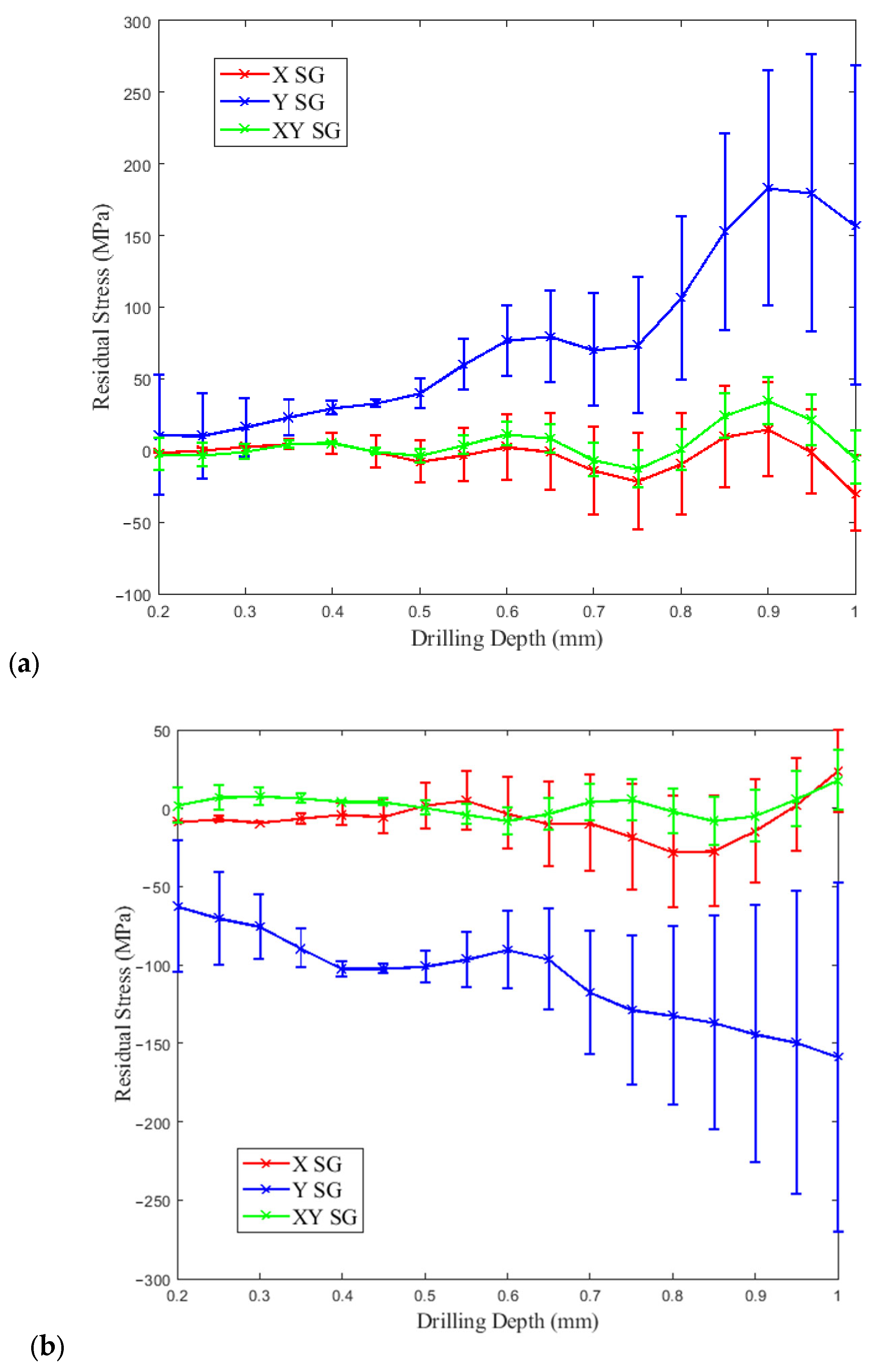
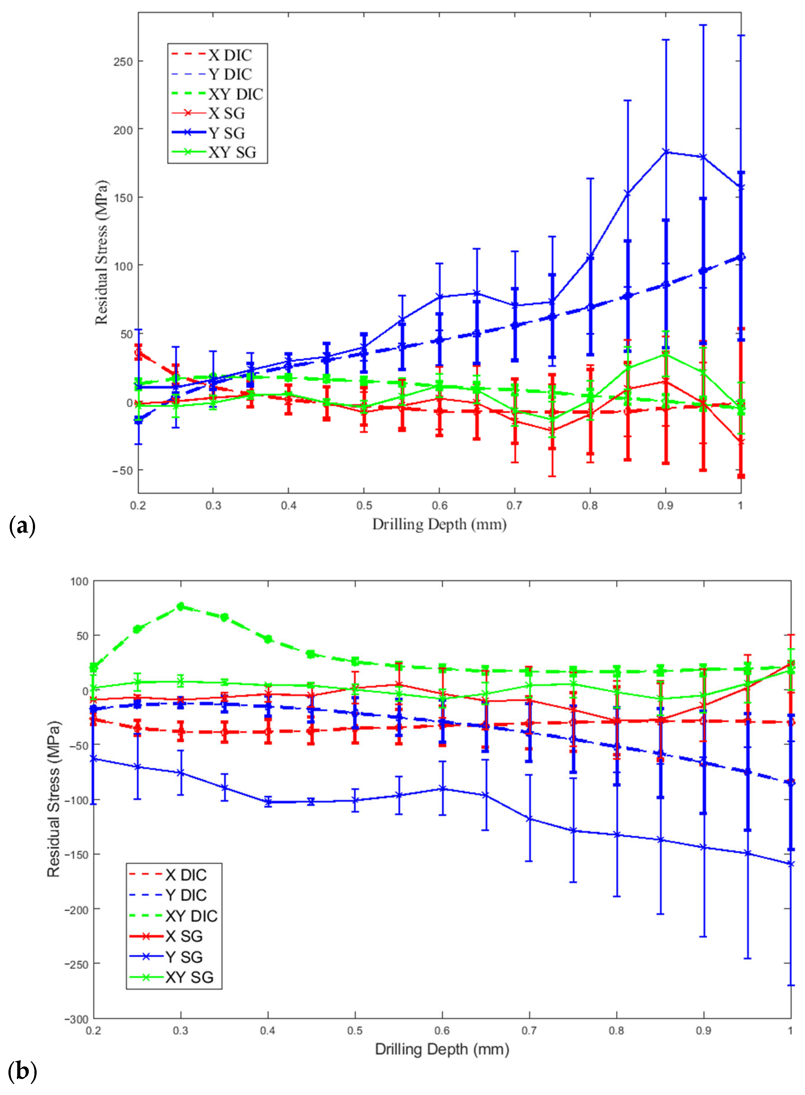
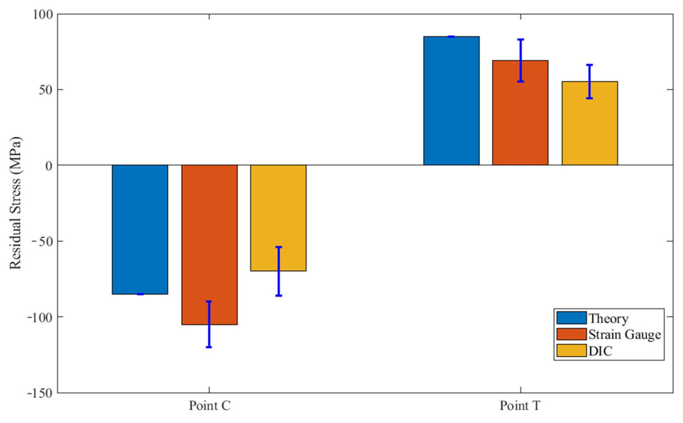
- Cross-validation of the methodology was performed on a test specimen using conventional methods and the results were found to be within +/−30 MPa.
- This device reduces measurement time from 2 h per point to 45 min and the cost of the experiment is reduced from £50 to £1 per measurement.
Abstract
1. Introduction
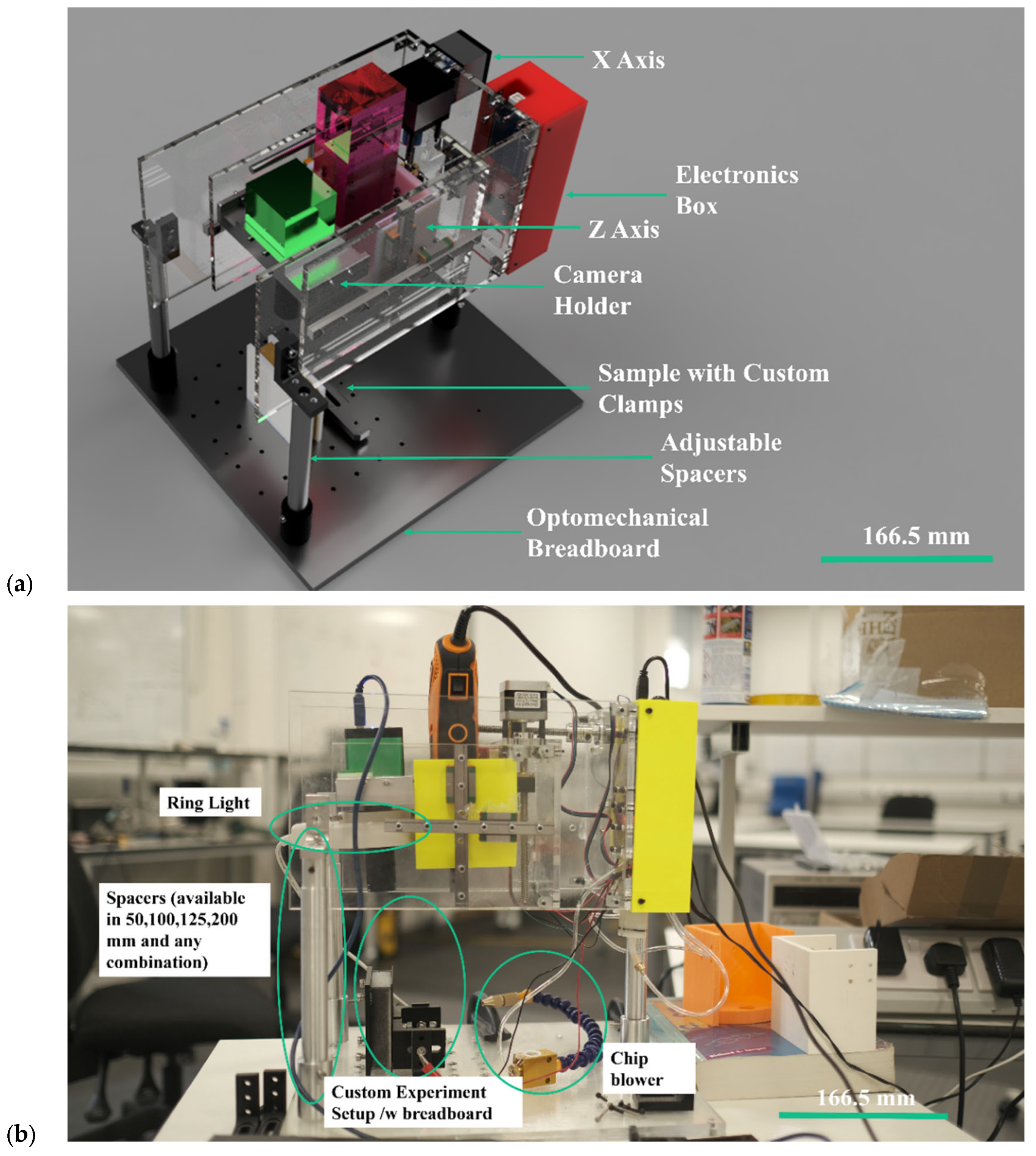
2. Device Design
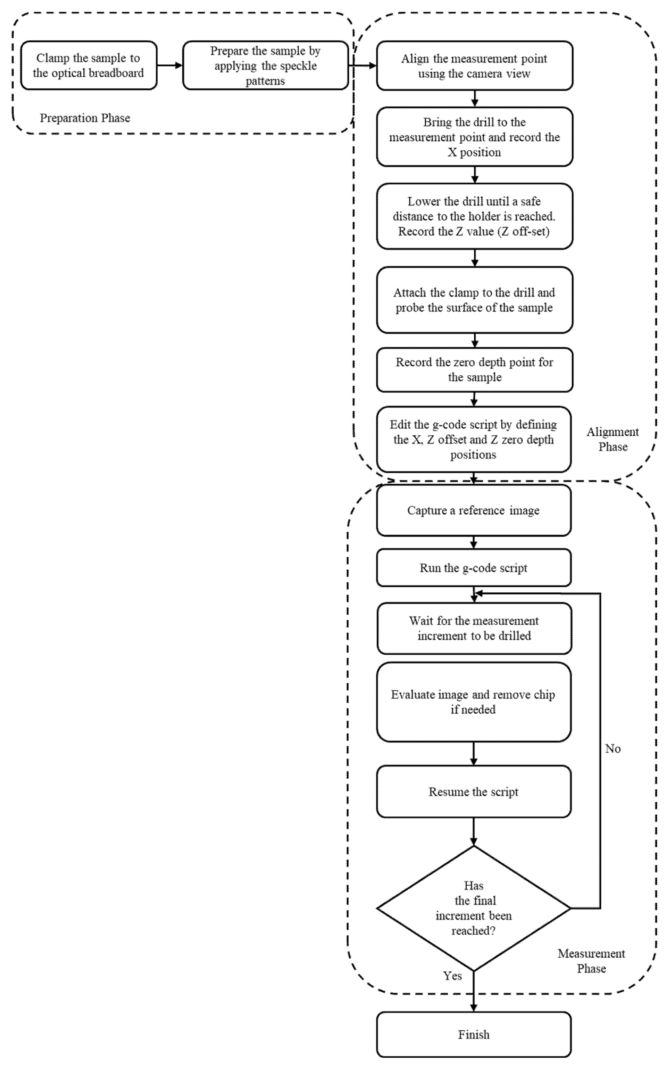
3. Experimental Procedure
3.1. Strain Gauge Calibration Measurements
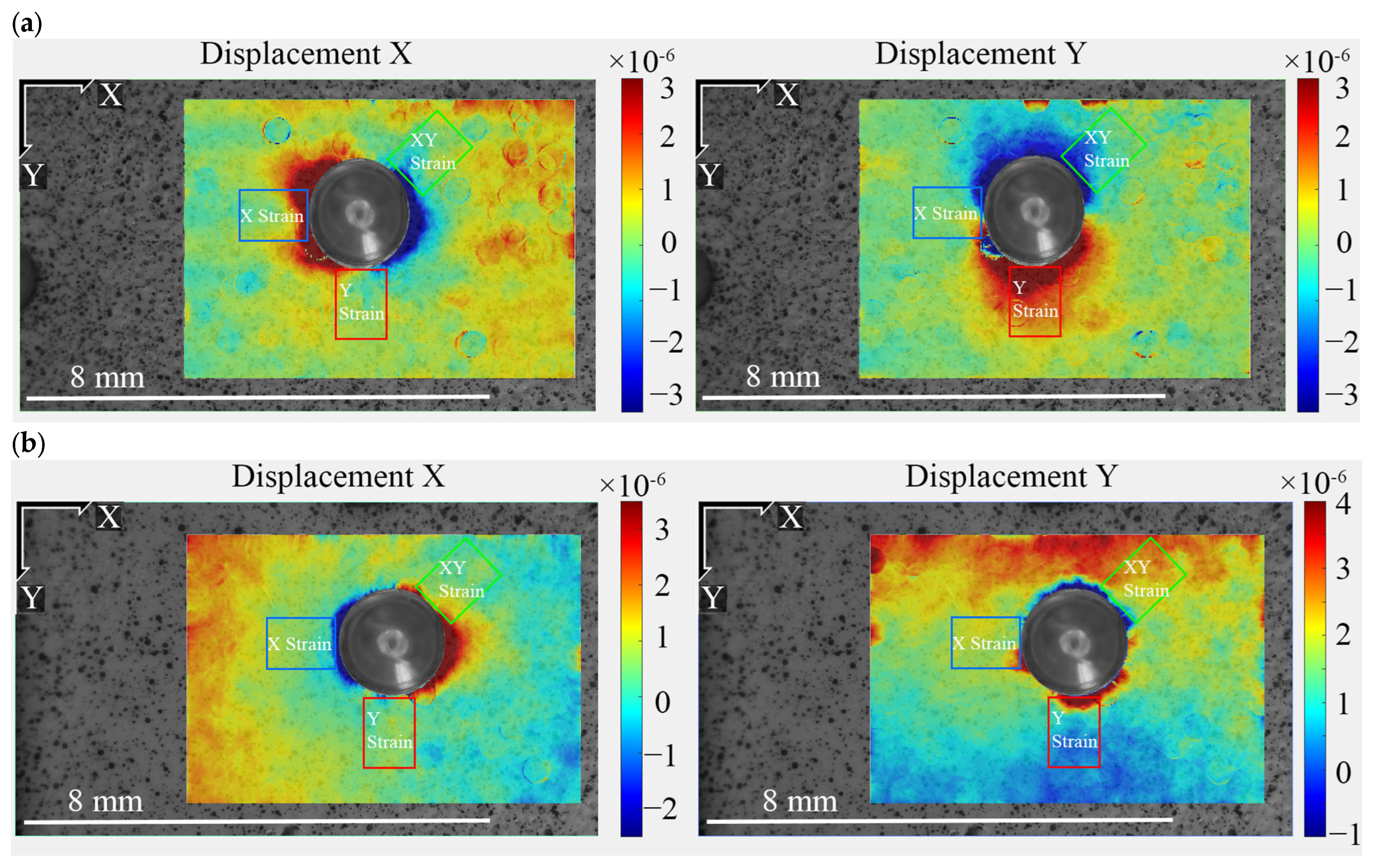
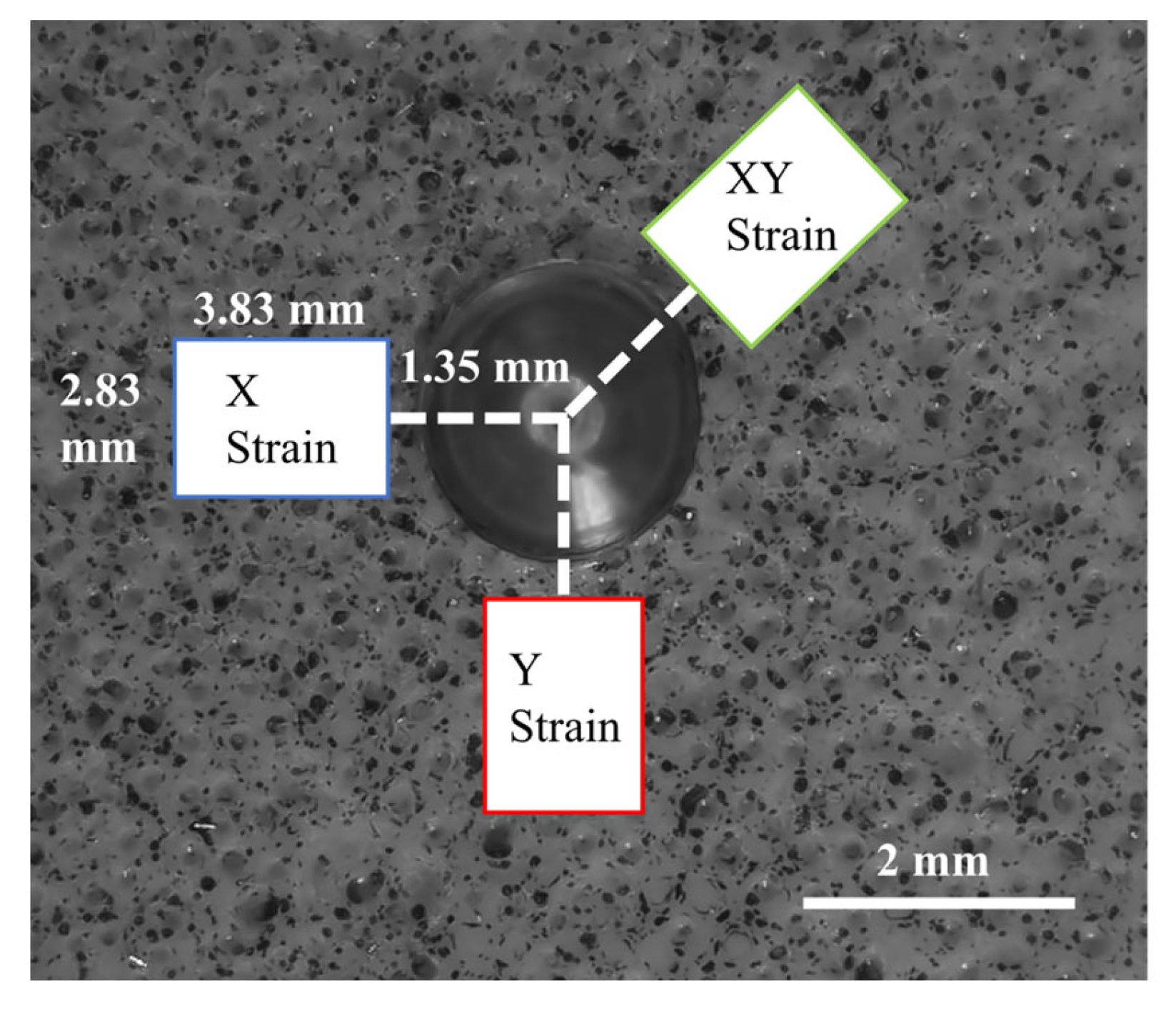
3.2. DIC-Based Measurements
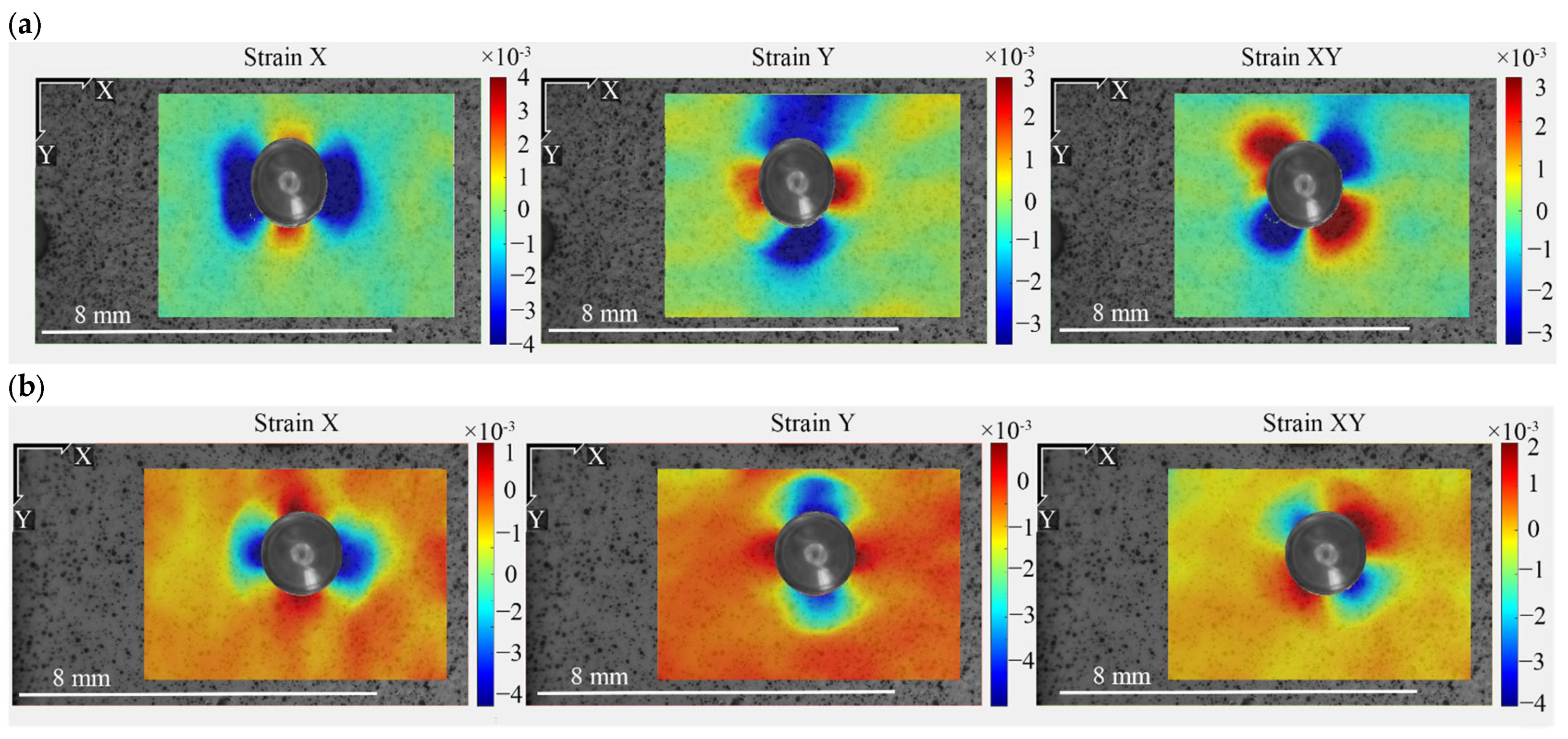
4. Results and Discussion
Device Performance Critique
- Ensure the sample is held securely. In this study, this was achieved by designing a range of sample holders specifically tailored to standard shapes/component designs. However, this is something that the user needs to keep in mind when performing this type of analysis, meaning that subsequent gripping methods may be required for non-standard geometries.
- Maximize the rigidity of the rig. Flexibility in the rig may lead to deformation of the rig/assembly during the milling/actuation process. Therefore, the design was specifically tailored and subsequently optimized in order to reduce deflection during these processes.
- Minimize the mass of the actuated components. Reducing the mass of the milling section of the rig reduces the force required by the motors in order to perform movements. Mass refinement was used extensively in the design of these sections of the device to ensure that the rig can be realigned to the highest precision possible.
- Make use of reliable references and a repeatable actuation system. An extensive design procedure was implemented to maximize this aspect of the design including the selection/use of lead screws, couplings, guides and suitable motors, as well as lubrication grease.
5. Conclusions
Supplementary Materials
Author Contributions
Funding
Institutional Review Board Statement
Informed Consent Statement
Data Availability Statement
Conflicts of Interest
Appendix A

Appendix B
References
- TWI. What is Residual Stress?—TWI. Available online: https://www.twi-global.com/technical-knowledge/faqs/residual-stress (accessed on 24 August 2021).
- Al-Turaihi, A.S. The Influence of Partial Peening on Fatigue Crack Growth. Ph.D. Thesis, Cranfield University, Cranfield, UK, 2017. [Google Scholar]
- Hanaki, T.; Hayashi, Y.; Akebono, H.; Kato, M.; Sugeta, A. Effect of compression Residual Stress on Fatigue Properties of Stainless Cast Steel. Procedia Struct. Integr. 2016, 2, 3143–3149. [Google Scholar] [CrossRef] [Green Version]
- Salvati, E.; Korsunsky, A.M. An analysis of macro- and micro-scale residual stresses of Type I, II and III using FIB-DIC micro-ring-core milling and crystal plasticity FE modelling. Int. J. Plast. 2017, 98, 123–138. [Google Scholar] [CrossRef]
- Liu, D.; Flewitt, P.E.J. Raman Measurements of Stress in Films and Coatings. Spectrosc. Prop. Inorg. Organomet. Compd. 2014, 45, 141–177. [Google Scholar] [CrossRef]
- Lunt, A.J.; Korsunsky, A.M. Intragranular Residual Stress Evaluation Using the Semi-Destructive FIB-DIC Ring-Core Drilling Method. Adv. Mater. Res. 2014, 996, 8–13. [Google Scholar] [CrossRef] [Green Version]
- James, M. Residual stress influences on structural reliability. Eng. Fail. Anal. 2011, 18, 1909–1920. [Google Scholar] [CrossRef]
- P. XRD. Residual Stress Information|Proto XRD, 2021. Available online: https://www.protoxrd.com/knowledge-center/residual-stress-info (accessed on 24 August 2021).
- Sim, W.-M. Residual Stress Engineering in Manufacture of Aerospace Structural Parts. In Proceedings of the 3rd International Conference on Distorsions Engineering, Bremen, Germany, 14–16 September 2011. [Google Scholar]
- Guo, J.; Fu, H.; Pan, B.; Kang, R. Recent progress of residual stress measurement methods: A review. Chin. J. Aeronaut. 2021, 34, 54–78. [Google Scholar] [CrossRef]
- Swain, D.; Sharma, A.; Selvan, S.; Thomas, B.; Govind; Philip, J. Residual stress measurement on 3-D printed blocks of Ti-6Al-4V using incremental hole drilling technique. Procedia Struct. Integr. 2019, 14, 337–344. [Google Scholar] [CrossRef]
- Li, C.; Liu, Z.; Fang, X.; Guo, Y. Residual Stress in Metal Additive Manufacturing. Procedia CIRP 2018, 71, 348–353. [Google Scholar] [CrossRef]
- Acevedo, R.; Sedlak, P.; Kolman, R.; Fredel, M. Residual stress analysis of additive manufacturing of metallic parts using ultrasonic waves: State of the art review. J. Mater. Res. Technol. 2020, 9, 9457–9477. [Google Scholar] [CrossRef]
- Mukherjee, T.; Zhang, W.; DebRoy, T. An improved prediction of residual stresses and distortion in additive manufacturing. Comput. Mater. Sci. 2017, 126, 360–372. [Google Scholar] [CrossRef] [Green Version]
- Czapski, P.; Kubiak, T. Influence of residual stresses on the buckling behaviour of thin-walled, composite tubes with closed cross-section—Numerical and experimental investigations. Compos. Struct. 2019, 229, 111407. [Google Scholar] [CrossRef]
- Negem, T. Residual Stress Analysis within Structures using Incremental hole-drilling. Master’s Thesis, TU Delft, Delft, The Netherlands, 2017. [Google Scholar]
- Rossini, N.; Dassisti, M.; Benyounis, K.; Olabi, A. Methods of measuring residual stresses in components. Mater. Des. 2012, 35, 572–588. [Google Scholar] [CrossRef] [Green Version]
- VEQTER. Overview|VEQTER|Residual Stress Experts, 2021. Available online: https://www.veqter.co.uk/residual-stress-measurement/overview (accessed on 24 August 2021).
- Kitano, H.; Okano, S.; Mochizuki, M. A study for high accuracy measurement of residual stress by deep hole drilling technique. J. Phys. Conf. Ser. 2012, 379, 012049. [Google Scholar] [CrossRef] [Green Version]
- Kingston, E.J. Advances in the Deep-Hole-Drilling Technique for Residual Stress Measurement. Ph.D. Thesis, University of Bristol, Bristol, UK, 2004. [Google Scholar]
- Sarga, P.; Menda, F. Comparison of Ring-Core Method and Hole-drilling Method Used for Determining Residual Stresses. Am. J. Mech. Eng. 2013, 1, 335–338. [Google Scholar] [CrossRef]
- Václavík, J.; Weinberg, O.; Bohdan, P.; Jankovec, J.; Holý, S. Evaluation of Residual Stresses using Ring Core Method. EPJ Web Conf. 2010, 6, 44004. [Google Scholar] [CrossRef] [Green Version]
- Chakrabarti, R.; Biswas, P.; Saha, S.C. A Review on Welding Residual Stress Measurement by Hole Drilling Technique and its Importance. J. Weld. Join. 2018, 36, 75–82. [Google Scholar] [CrossRef] [Green Version]
- Barile, C.; Casavola, C.; Pappalettera, G.; Pappalettere, C. Remarks on Residual Stress Measurement by Hole-Drilling and Electronic Speckle Pattern Interferometry. Sci. World J. 2014, 2014, 3. [Google Scholar] [CrossRef] [PubMed] [Green Version]
- Lothhammer, L.R.; Viotti, M.R.; Albertazzi, A., Jr.; Veiga, C.L. Residual stress measurements in steel pipes using DSPI and the hole-drilling technique. Int. J. Press. Vessel. Pip. 2017, 152, 46–55. [Google Scholar] [CrossRef]
- Schajer, G.S. Practical Residual Stress Measurement Methods; John Wiley & Sons: Hoboken, NJ, USA, 2013; pp. 1–310. [Google Scholar] [CrossRef]
- Niku-Lari, A.; Lu, J.A.; Flavenot, J.F. Measurement of Residual Stress Distribution by the Incremental Hole-Drilling Method. J. Mech. Work. Technol. 1985, 11, 167–188. [Google Scholar] [CrossRef]
- Bigger, R.; Blaysat, B.; Boo, C.; Grewer, M.; Hu, J.; Jones, A.; Klein, M.; Raghavan, K.; Reu, P.; Schmidt, T.; et al. A Good Practices Guide for Digital Image Correlation. Volume 5. International Digital Image Correlation Society. 2018. Available online: https://idics.org/guide/DICGoodPracticesGuide_PrintVersion-V5h-181024.pdf (accessed on 15 March 2022).
- Baldi, A. Residual Stress Measurement Using Hole Drilling and Integrated Digital Image Correlation Techniques. Exp. Mech. 2013, 54, 379–391. [Google Scholar] [CrossRef]
- Sabate, N.; Vogel, D.; Gollhardt, A.; Keller, J.; Cane, C.; Gracia, I.; Morante, J.R.; Michel, B. Residual Stress Measurement on a MEMS Structure With High-Spatial Resolution. J. Microelectromech. Syst. 2007, 16, 365–372. [Google Scholar] [CrossRef] [Green Version]
- Lunt, A.J.G.; Korsunsky, A.M. A review of micro-scale focused ion beam milling and digital image correlation analysis for residual stress evaluation and error estimation. Surf. Coat. Technol. 2015, 283, 373–388. [Google Scholar] [CrossRef]
- Yang, L. Measure Strain Distribution Using Digital Image Correlation (DIC) for Tensile Tests Final Report; The Advanced High Strength Steel Stamping Team of the Auto/Steel Partnership: Southfield, MI, USA, 2010. [Google Scholar]
- Botean, A.-I. Thermal expansion coefficient determination of polylactic acid using digital image correlation. E3S Web Conf. 2018, 32, 01007. [Google Scholar] [CrossRef] [Green Version]
- Steinzig, M.; Ponslet, E. Residual stress measurement using the hole drilling method and laser speckle interferometry: Part 1. Exp. Tech. 2003, 27, 43–46. [Google Scholar] [CrossRef]
- Lord, J.D.; Penn, D.; Whitehead, P. The Application of Digital Image Correlation for Measuring Residual Stress by Incremental Hole Drilling. Appl. Mech. Mater. 2008, 13–14, 65–73. [Google Scholar] [CrossRef] [Green Version]
- Lee, J.; Jeong, S.; Lee, Y.-J.; Sim, S.-H. Stress Estimation Using Digital Image Correlation with Compensation of Camera Motion-Induced Error. Sensors 2019, 19, 5503. [Google Scholar] [CrossRef] [Green Version]
- Harrington, J.S.; Schajer, G.S. Measurement of Structural Stresses by Hole-Drilling and DIC. Exp. Mech. 2016, 57, 559–567. [Google Scholar] [CrossRef]
- Krottenthaler, M.; Schmid, C.; Schaufler, J.; Durst, K.; Göken, M. A simple method for residual stress measurements in thin films by means of focused ion beam milling and digital image correlation. Surf. Coat. Technol. 2013, 215, 247–252. [Google Scholar] [CrossRef]
- Kandil, F.A.; Lord, J.D.; Fry, A.T.; Grant, P.V. A review of residual stress measurement methods—A guide to technical selection. NPL Mater. Cent. 2001, 4, 1–42. [Google Scholar]
- Arabul, E. Hole-Drilling and Digital Image Correlation for Residual Stress Analysis; Design and Production of a Novel Microscope and Milling Rig. Master’s Thesis, University of Bath, Bath, UK, 2021. [Google Scholar]
- VEQTER. Synchrotron Diffraction. 2022. Available online: https://www.veqter.co.uk/residual-stress-measurement/synchrotron-diffraction (accessed on 15 March 2022).
- Vishay Precision Group. Measurement of Residual Stresses by the Hole-Drilling Strain-Gage Method, Tech Note TN-503′. 2007. Available online: http://www.vishaypg.com/docs/11053/tn503 (accessed on 15 March 2022).
- SINT Technology. Residual Stress Measurement-Restan MTS3000. 2021. Available online: https://www.mts3000.com/mts3000-restan/ (accessed on 15 March 2022).
- Inc Correlated Solutions. Vic-3D Stereo Microscope-isi-sys. 2020. Available online: http://www.isi-sys.com/vic-3d-micro-system/ (accessed on 15 March 2022).
- Stresstech. ESPI Hole-drilling-Stresstech. Available online: https://www.stresstech.com/knowledge/semi-destructive-testing-methods/espi-hole-drilling/ (accessed on 15 March 2022).
- Pástor, M.; Hagara, M.; Virgala, I.; Kal’Avský, A.; Sapietová, A.; Hagarová, L. Design of a Unique Device for Residual Stresses Quantification by the Drilling Method Combining the PhotoStress and Digital Image Correlation. Materials 2021, 14, 314. [Google Scholar] [CrossRef]
- Ajovalasit, A. Measurement of residual stresses by the hole-drilling method: Influence of hole eccentricity. J. Strain Anal. Eng. Des. 1979, 14, 171–178. [Google Scholar] [CrossRef]
- Beghini, M.; Bertini, L.; Mori, L.F. Evaluating Non-Uniform Residual Stress by the Hole-Drilling Method with Concentric and Eccentric Holes. Part I. Definition and Validation of the Influence Functions. Strain 2010, 46, 324–336. [Google Scholar] [CrossRef]
- Barsanti, M.; Beghini, M.; Bertini, L.; Monelli, B.D.; Santus, C. First-order correction to counter the effect of eccentricity on the hole-drilling integral method with strain-gage rosettes. J. Strain Anal. Eng. Des. 2016, 51, 431–443. [Google Scholar] [CrossRef] [Green Version]
- Reu, P.L.; Sweatt, W.C.; Miller, T.J.; Fleming, D. Camera System Resolution and its Influence on Digital Image Correlation. Exp. Mech. 2014, 55, 9–25. [Google Scholar] [CrossRef]
- Lecompte, D.; Academy, R.M.; Cooreman, S.; Sol, H.; Brussel, V.U. Study and generation of optimal speckle patterns for DIC Study and generation of optimal speckle patterns for DIC. In Proceedings of the Annual Conference and Exposition on Experimental and Applied mechanics, Springfield, MA, USA, 3–6 June 2007. [Google Scholar]
- Hohmann, B.P.; Bruck, P.; Esselman, T.C.; Schmidt, T. Digital Image Correlation (DIC): An Advanced Nondestructive Testing Method for Life Extension of Nuclear Power Plants; International Atomic Energy Agency (IAEA): Vienna, Austria, 2012; pp. 1–8. [Google Scholar]
- Haddadi, H.; Belhabib, S. Use of rigid-body motion for the investigation and estimation of the measurement errors related to digital image correlation technique. Opt. Lasers Eng. 2008, 46, 185–196. [Google Scholar] [CrossRef]
- Rickert, T. Hole Drilling With Orbiting Motion for Residual Stress Measurement—Effects of Tool and Hole Diameters. SAE Int. J. Engines 2017, 10, 467–470. [Google Scholar] [CrossRef]
- Schreier, H.; Orteu, J.-J.; Sutton, M.A. Image Correlation for Shape, Motion and Deformation Measurements: Basic Concepts, Theory and Applications; Springer Science & Business Media: Boston, MA, USA, 2009. [Google Scholar] [CrossRef]
- Jeon, S.K. Grbl. 2021. Available online: https://github.com/grbl/grbl (accessed on 15 March 2022).
- Yang, Q.-M.; Lee, Y.-S.; Lee, E.-Y.; Kim, J.-H.; Cha, K.-U.; Hong, S.-K. A residual stress analysis program using a Matlab GUI on an autofrettaged compound cylinder. J. Mech. Sci. Technol. 2009, 23, 2913–2920. [Google Scholar] [CrossRef]
- Quino, G.; Chen, Y.; Ramakrishnan, K.R.; Martínez-Hergueta, F.; Zumpano, G.; Pellegrino, A.; Petrinic, N. Speckle patterns for DIC in challenging scenarios: Rapid application and impact endurance. Meas. Sci. Technol. 2020, 32, 015203. [Google Scholar] [CrossRef]
- Szalai, S.; Dogossy, G. Speckle pattern optimization for DIC technologies. Acta Technol. Jaurinensis 2021, 14, 228–243. [Google Scholar] [CrossRef]
- Begonia, M.; Dallas, M.; Johnson, M.L.; Thiagarajan, G. Comparison of strain measurement in the mouse forearm using subject-specific finite element models, strain gaging, and digital image correlation. Biomech. Model. Mechanobiol. 2017, 16, 1243–1253. [Google Scholar] [CrossRef]
- Lord, J.; Cox, D.; Ratzke, A. A Good Practice Guide for Measuring Residual Stresses Using FIB-DIC, The National Physical Laboratory (NPL). 2018. Available online: https://eprintspublications.npl.co.uk/7807/1/MGPG143 (accessed on 7 April 2021).
- Sijbers, J.; Scheunders, P.; Bonnet, N. Quantification and Improvement of the Signal-to-Noise Ratio in a Magnetic Resonance Image Acquisition Procedure. Magn. Reson. Imaging 1996, 14, 1157–1163. [Google Scholar] [CrossRef]
- Blaber, J.A.A. Ncorr-Instruction Manual Version 1.2.2-Master. 2017. Available online: http://www.ncorr.com/download/ncorrmanual_v1_2_2 (accessed on 15 March 2022).
- Schajer, G.S. Optical Hole-Drilling Residual Stress Calculations Using Strain Gauge Formalism. Exp. Mech. 2021, 61, 1369–1380. [Google Scholar] [CrossRef]
- Barsanescu, P.; Carlescu, P. Residual Stress Measurement by the Hole-Drilling Strain-Gage Method: Influence of Hole Eccentricity; Technical University: Iasi, Romania, 2007. [Google Scholar]
- Návrat, T.; Halabuk, D.; Vlk, M.; Vosynek, P. Eccentricity Effect in the Hole-Drilling Residual Stress Measurement. Defect Diffus. Forum 2018, 382, 208–212. [Google Scholar] [CrossRef]
- Ajovalasit, A.; Scafidi, M.; Zuccarello, B.; Beghini, M.; Bertini, L. The Hole-Drilling Strain Gauge Method for the Measurement of Uniform or Non-Uniform Residual Stresses; Working Group on Residual Stresses; University of Palermo: Palermo, Italy, 2010; pp. 1–70. [Google Scholar]
- Grant, P.V.; Lord, J.D.; Whitehead, P.S. Measurement Good Practice Guide No. 53 The Measurement of Residual Stresses by the Incremental Hole-drilling Technique. 2002. Available online: https://eprintspublications.npl.co.uk/2517/1/mgpg53.pdf (accessed on 15 March 2022).
- Schajer, G.S. Advances in Hole-Drilling Residual Stress Measurements. Exp. Mech. 2009, 50, 159–168. [Google Scholar] [CrossRef]
- Viksne, A. Residual Stress Measurement of 7050 Aluminum Alloy Open Die Forgings Using the Hole-Drilling Method by Approval Page. Bachelor Thesis, California Polytechnic State University, San Luis Obispo, CA, USA, 2013. [Google Scholar]
- Revie, R.W. Residual Stress in Pipelines. Oil and Gas Pipelines: Integrity and Safety Handbook, 1st ed.; CANMET Materials Technology Laboratory: Ottawa, ON, Canada, 2015. [Google Scholar]
- Mirzaee-Sisan, A.; Wu, G. Residual stress in pipeline girth welds- A review of recent data and modelling. Int. J. Press. Vessel. Pip. 2018, 169, 142–152. [Google Scholar] [CrossRef]
- Surface Preparation for Strain Gage Bonding Instruction Bulletin B-129-8 Surface Preparation for Strain Gage Bonding. Available online: www.micro-measurements.com (accessed on 26 August 2021).
- ASTM E837-20. Standard Test Method for Determining Residual Stresses by the Hole-Drilling Strain-Gages. Available online: https://www.astm.org/e0837-20.html (accessed on 15 March 2022).
- Schajer, G.S. Measurement of Non-Uniform Residual Stresses Using the Hole-Drilling Method—Part I: Stress Calculation Procedure; Materials Division (Publication) MD 7; American Society of Mechanical Engineers, Weyerhaeuser Technology Center: Tacoma, WA, USA, 1988; pp. 85–91. [Google Scholar]
- Schajer, G.S. Measurement of Non-Uniform Residual Stresses Using the Hole-Drilling Method. Part II-Practical Application of the Integral Method; American Society of Mechanical Engineers, Weyerhaeuser Technology Center: Tacoma, WA, USA, 1988. [Google Scholar]


| Strain Gauges | DIC |
|---|---|
| Measurement errors: | |
| Errors due to misalignment between drilled hole and strain gauge rosette | No requirement for exact drilling-hole alignment relative to the sensor (as long as it remains in the field of view) |
| Manual application of strain gauges may lead to imprecision in location, contact effectiveness, etc. | Repeatable measurements at the location of interest—alignment performed digitally |
| Type of strain: | |
| Single point measurement of strain—averaging over a region | Full-field strain and deformation measurement |
| Unable to quantify stress state in inhomogeneous or anisotropic materials | Full-field residual stress data, suitable for inhomogeneous and anisotropic materials |
| Economical aspects: | |
| High cost per measurement (£50+) | Low operation cost per measurement (£1) |
| Preparation time for applying the strain gauge (Est. 2 h per point) | Fast and simple preparation of object surface(45 min per measurement) |
| Specifications | Details |
|---|---|
| Complete measurement process | The device and the associated software take the user through the complete measurement process. |
| Fast measurements | Each measurement takes around 25 min with 45 min of preparation. |
| Low cost per measurement | Significantly reduces the cost of measurement by requiring minimal preparation. |
| Non-contact measurements | The surface of the material is minimally disturbed when making measurements e.g., via the addition of strain gauges. |
| Fit for lab use | Able to make measurements for different applications (materials research, aerospace etc.). |
| Precise hole positioning and incremental drilling | Able to drill actuate both axes to a resolution of 0.05 mm. |
| Zero-point detection | The device can detect the zero depth of the work sample. |
| Flexible Sample Size | Can accommodate multiple sample sizes via flexible clamping. |
| A low level of expertise needed | The device and the associated software do not require specialised knowledge to operate. |
| Evaluation process integrated | The device evaluates the results of residual stress measurements. |
| Comparable to ASTM E837-E13a | The results are comparable to ASTM E837-E13a, the hole-drilling method measurement standard. |
| Aimed towards the lower-midrange market | The device costs £380. |
| Open-sourced | Documentation for the device is open-sourced. |
| Semi-Automatic Mode |
|---|
| 1: G28.1; Set the absolute home position |
| 2: M8; Start chip blower |
| 3: G1 X position Z position F feed rate; Move to the predefined drilling position, defined by the user |
| 4: G91; Switch to incremental drilling mode |
| 5: G30.1; Redefine the current position as the secondary home position |
| 6: G1 Z position; Lower drill over the hole based on the zero-point measurement |
| 7: G1; Drill the increment, allowing for dwell to ensure the hole is formed |
| 8: G30; Move the drill back to the secondary home position |
| 9: G28; Return to the absolute home position, align the DIC camera over the sample |
| 10: M0; Wait for user input to continue drilling, once the satisfactory images are captured |
| 11: Repeat steps 3–10 process until the desired hole depth is achieved |
| No. | Subsystem | Quantity | Part Name | Cost Per Piece (£) | Total Cost (£) |
|---|---|---|---|---|---|
| 1 | DIC System | 1 | HAYEAR 48 MP Microscope Camera + 100× C-mount Lens + 56 LED Ring Light For Soldering Repair + Stand Holder | 108.55 | 108.55 |
| 2 | Drilling System | 1 | TACKLIFE Rotary Tool Kit | 35.99 | 35.99 |
| 3 | 1 | 1.6 mm Tungsten Carbide PCB Drill Bit | 8.59 | 8.59 | |
| 4 | Speckle Pattern Application | 1 | Plasti-kote 3101 400 mL Super Spray Paint-Matt Black | 5.02 | 5.02 |
| 5 | 1 | Plasti-kote 3100SE 400 mL Super Matt Spray Paint-White | 5.02 | 5.02 | |
| 6 | The Actuation | 2 | T8 Trapezoidal Lead Screw Lead Screw + T8 Nut | 8.99 | 17.98 |
| 7 | 2 | 5 mm to 8 mm Shaft Coupling | 6.49 | 12.98 | |
| 8 | 2 | Nema 17 Stepper Motor | 10.00 | 20 | |
| 9 | 4 | LML12B Miniature Linear Rail Guide 150 | 7.99 | 31.96 | |
| 10 | 2 | EasyDriver Shield Stepper Motor Driver | 5.99 | 11.98 | |
| 11 | 1 | Mechanical Endstop Limit Switch | 6.99 | 6.99 | |
| 12 | 1 | Arduino Uno | 9.99 | 9.99 | |
| 13 | 1 | Lithium Grease | 5.06 | 5.06 | |
| 14 | Zero Depth Detection | 1 | Alligator Clips Clamps | 1.99 | 1.99 |
| 15 | Sample Attachment | 1 | 52 mm suction cup with M4 screw | 6.49 | 6.49 |
| 16 | Packaging | 26 | RS PRO 15 × 15 mm 2 Hole Steel Angle Bracket | 0.183 | 4.76 |
| 17 | 1 | RS PRO M3 × 12 mm Hex Socket Cap Screw Black, Self-Colour Steel (Pack of 100) | 13.98 | 13.98 | |
| 18 | 1 | RS PRO Steel, Hex Nut, M3 | 4.02 | 4.02 | |
| 19 | 1 | Zinc Plated Steel Plain Washer, 0.5 mm Thickness, M3 | 1.11 | 1.11 | |
| 20 | 1 | Manufacturing Expenses | 50 | 50 | |
| Total Cost | 362.46 |
| Category | Parameter | Selected Value |
|---|---|---|
| Experimental Setup | Image Resolution and Frame Rate | 2.7 k @ 30 FPS |
| Speckle Pattern Density | 3–7 Pixels, with a target of 50% | |
| Image Format | 8 bit, TIFF | |
| Illumination used | Ring light, perpendicular to the sample | |
| Pre-processing | Images Averaged | 25 images each increment |
| Rigid Body Compensation | Yes, the first image reference | |
| DIC Settings | Image Region Analysed | 3 × 3 mm section surrounding the drilled hole |
| Correlation Subset Radius | 48 pixels, circular section | |
| Subset Spacing | 2 pixels | |
| DIC Calculation Algorithm | Inverse compositional method [63] | |
| Residual Stress Estimation | Calibration Factors | Adjusted for the DIC method and hole size |
| Hole Diameter | 2 mm | |
| Youngs Modulus | 70 GPa | |
| Poisson Ratio | 0.33 |
Publisher’s Note: MDPI stays neutral with regard to jurisdictional claims in published maps and institutional affiliations. |
© 2022 by the authors. Licensee MDPI, Basel, Switzerland. This article is an open access article distributed under the terms and conditions of the Creative Commons Attribution (CC BY) license (https://creativecommons.org/licenses/by/4.0/).
Share and Cite
Arabul, E.; Lunt, A.J.G. A Novel Low-Cost DIC-Based Residual Stress Measurement Device. Appl. Sci. 2022, 12, 7233. https://doi.org/10.3390/app12147233
Arabul E, Lunt AJG. A Novel Low-Cost DIC-Based Residual Stress Measurement Device. Applied Sciences. 2022; 12(14):7233. https://doi.org/10.3390/app12147233
Chicago/Turabian StyleArabul, Ege, and Alexander J. G. Lunt. 2022. "A Novel Low-Cost DIC-Based Residual Stress Measurement Device" Applied Sciences 12, no. 14: 7233. https://doi.org/10.3390/app12147233
APA StyleArabul, E., & Lunt, A. J. G. (2022). A Novel Low-Cost DIC-Based Residual Stress Measurement Device. Applied Sciences, 12(14), 7233. https://doi.org/10.3390/app12147233