
A Hybrid Firefly–JAYA Algorithm for the Optimal Power Flow Problem Considering Wind and Solar Power Generations


Abstract
:1. Introduction
2. Problem Formulation
2.1. OPF Constraints
2.1.1. OPF Equality Constraints
2.1.2. OPF Inequality Constraints
- Constraints relating to the generation units: for all the generators, the voltage, as well as the reactive and active powers, should be defined in upper and lower limits as follows:
- Transformers’ tap adjustments: transformers’ taps can be altered in their approved limitation as in [13]:
- Constraints of VAR compensating units: the productions of these units are constrained in the following way [13]:
- Voltage limits: the acceptable range of load bus voltage magnitudes are known as a security constraint [13]:
- Transmission lines constraints: the apparent power flows across branches should be restricted by:
3. Proposed Mix Optimizer
3.1. Firefly Algorithm (FA)
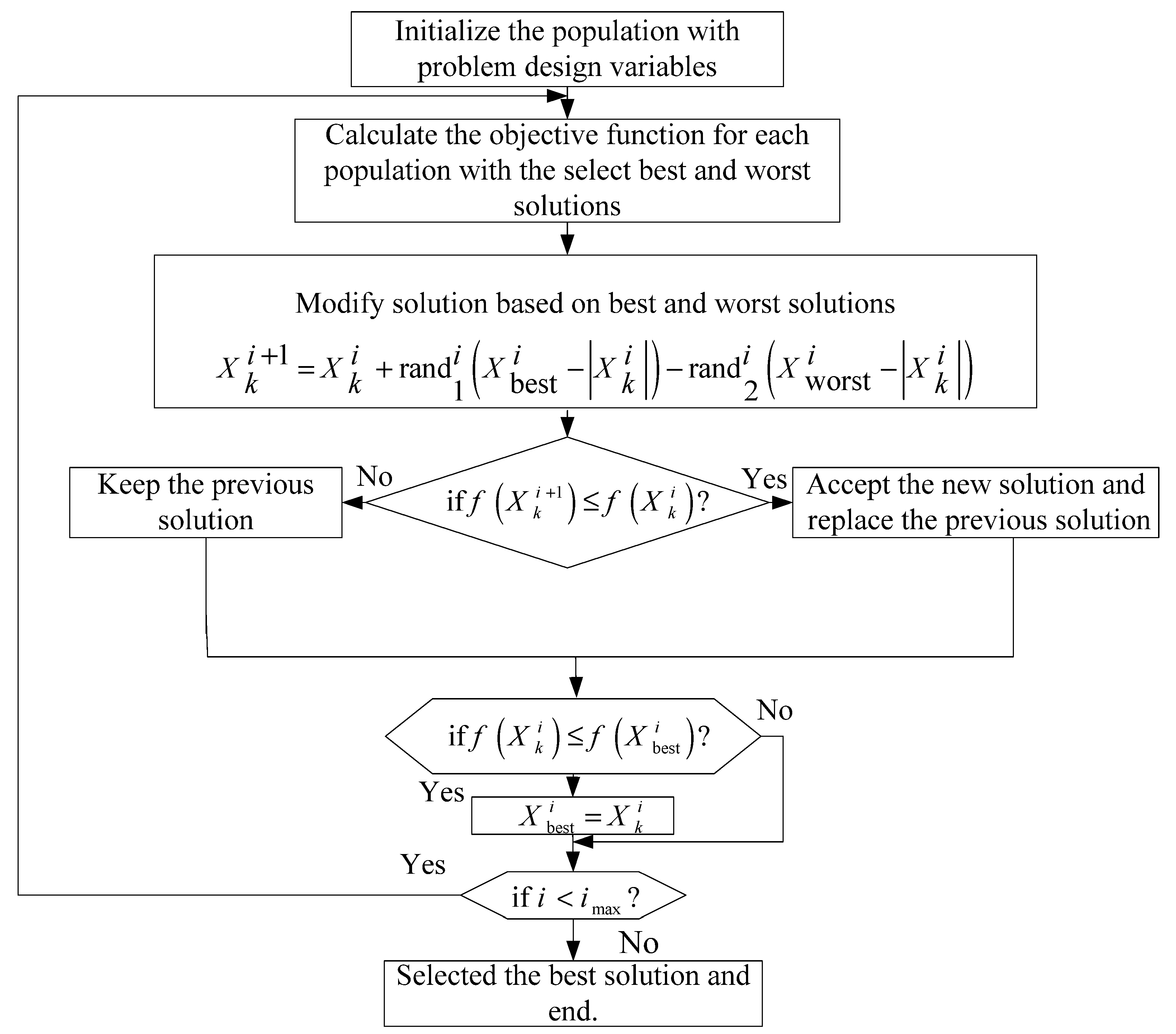
3.2. JAYA Algorithm
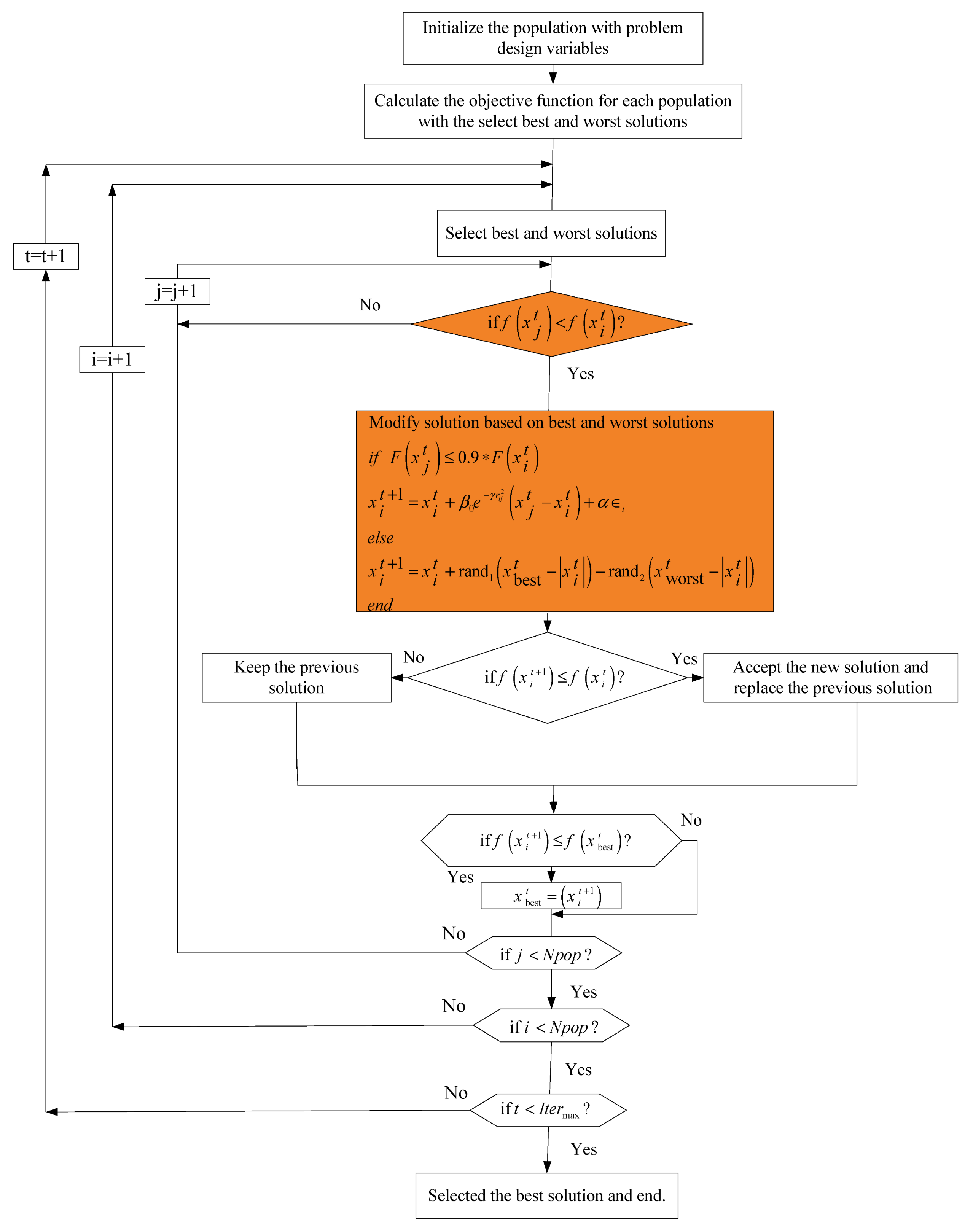
3.3. The Proposed HFAJAYA Optimization Algorithm
4. HFAJAYA for the Multi-Constraint OPF Problems
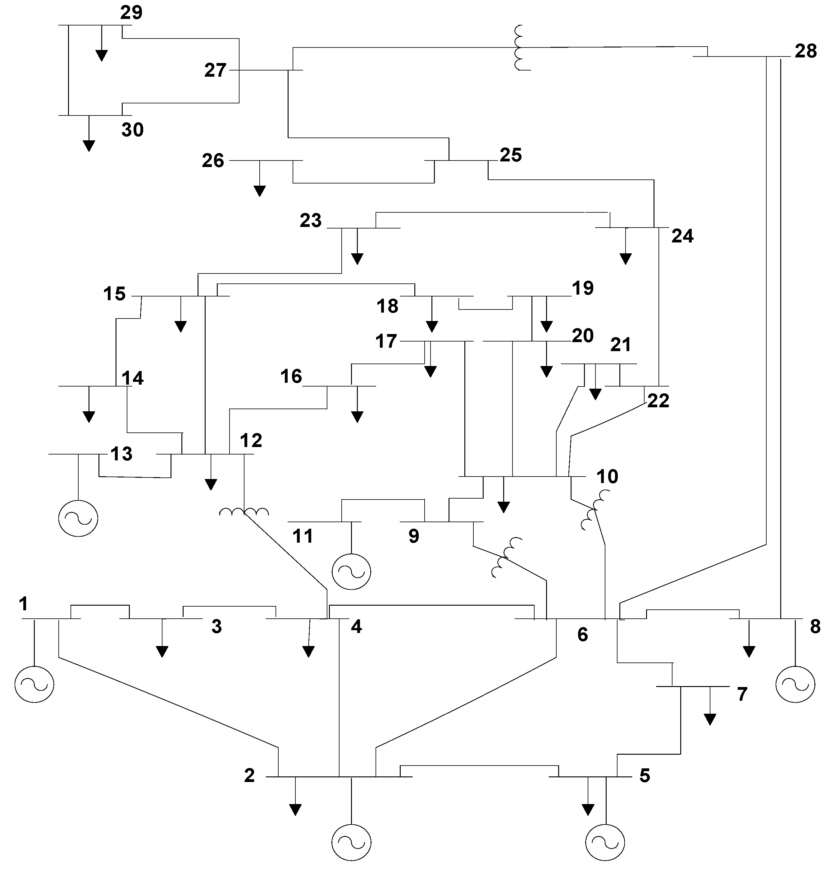
- The considered cases for the IEEE 30-bus system:
4.1. OPF without Stochastic Renewable Energy
4.1.1. Case 1
4.1.2. Case 2
4.1.3. Case 3
4.1.4. Case 4
4.1.5. Case 5
4.1.6. Case 6
4.2. OPF Solutions, Including Stochastic Solar and Wind Power
4.2.1. The Mathematical Modeling of Generating Units, Including Solar and Wind Power
4.2.2. The Units of Wind Power
4.2.3. Solar Power Units
4.2.4. Case 7
4.2.5. Case 8
4.3. Discussion on Results
5. Conclusions
Funding
Institutional Review Board Statement
Informed Consent Statement
Data Availability Statement
Acknowledgments
Conflicts of Interest
Appendix A

| Generator Number | α | b | c | d | e | PGmax | PGmin | Prohibit Zones | |
|---|---|---|---|---|---|---|---|---|---|
| PG1 (MW) | 0.0 | 2 | 0.00375 | 18 | 0.037 | 250 | 50 | [55, 66], [80, 120] | |
| PG2 (MW) | 0.0 | 1.75 | 0.0175 | 16 | 0.038 | 80 | 20 | [21, 24], [45, 55] | |
| PG5 (MW) | 0.0 | 1.0 | 0.0625 | 14 | 0.04 | 50 | 15 | [30, 36] | |
| PG8 (MW) | 0.0 | 3.25 | 0.00834 | 12 | 0.045 | 35 | 10 | [25, 30] | |
| PG11 (MW) | 0.0 | 3 | 0.025 | 13 | 0.042 | 30 | 10 | [25, 28] | |
| PG13 (MW) | 0.0 | 3 | 0.025 | 13.5 | 0.041 | 40 | 12 | [24, 30] | |
| Generator Number | Form MW | To MW | Cost Coefficients | ||
|---|---|---|---|---|---|
| α | b | c | |||
| PG1 (MW) | 50 | 140 | 55 | 0.7 | 0.005 |
| 140 | 200 | 82.5 | 1.05 | 0.0075 | |
| PG2 (MW) | 20 | 55 | 40 | 0.3 | 0.01 |
| 55 | 80 | 80 | 0.6 | 0.02 | |
| Emission Coefficients | ||||||
|---|---|---|---|---|---|---|
| γ | 0.0649 | 0.05638 | 0.04586 | 0.0338 | 0.04586 | 0.05151 |
| β | −0.05554 | −0.06047 | −0.05094 | −0.0355 | −0.05094 | −0.05555 |
| α | 0.04091 | 0.02543 | 0.04258 | 0.05326 | 0.04258 | 0.06131 |
| ξ | 0.0002 | 0.0005 | 0.000001 | 0.002 | 0.000001 | 0.00001 |
| λ | 2.857 | 3.333 | 8 | 2 | 8 | 6.667 |
References
- Roy, P.K.; Ghoshal, S.P.; Thakur, S.S. Biogeography Based Optimization for Multi-Constraint Optimal Power Flow with Emission and Non-Smooth Cost Function. Expert Syst. Appl. 2010, 37, 8221–8228. [Google Scholar] [CrossRef]
- Alanazi, M.S. A Modified Teaching—Learning-Based Optimization for Dynamic Economic Load Dispatch Considering Both Wind Power and Load Demand Uncertainties with Operational Constraints. IEEE Access 2021, 9, 101665–101680. [Google Scholar] [CrossRef]
- Surender Reddy, S.; Srinivasa Rathnam, C. Optimal Power Flow Using Glowworm Swarm Optimization. Int. J. Electr. Power Energy Syst. 2016, 80, 128–139. [Google Scholar] [CrossRef]
- Alghamdi, A.S. Optimal Power Flow of Renewable-Integrated Power Systems Using a Gaussian Bare- Bones Levy-Flight Firefly Algorithm. Front. Energy Res. 2022, 10, 921936. [Google Scholar] [CrossRef]
- Alghamdi, A.S. A New Self-Adaptive Teaching–Learning-Based Optimization with Different Distributions for Optimal Reactive Power Control in Power Networks. Energies 2022, 15, 2759. [Google Scholar] [CrossRef]
- Duman, S.; Li, J.; Wu, L. AC Optimal Power Flow with Thermal-Wind-Solar-Tidal Systems Using the Symbiotic Organisms Search Algorithm. IET Renew. Power Gener. 2021, 15, 278–296. [Google Scholar] [CrossRef]
- Duman, S.; Wu, L.; Li, J. Moth Swarm Algorithm Based Approach for the ACOPF Considering Wind and Tidal Energy. In Proceedings of the International Conference on Artificial Intelligence and Applied Mathematics in Engineering, Antalya, Turkey, 20–22 April 2019; Springer: Berlin/Heidelberg, Germany, 2019; pp. 830–843. [Google Scholar]
- Elattar, E.E. Optimal Power Flow of a Power System Incorporating Stochastic Wind Power Based on Modified Moth Swarm Algorithm. IEEE Access 2019, 7, 89581–89593. [Google Scholar] [CrossRef]
- Mohamed, A.-A.A.; Mohamed, Y.S.; El-Gaafary, A.A.M.; Hemeida, A.M. Optimal Power Flow Using Moth Swarm Algorithm. Electr. Power Syst. Res. 2017, 142, 190–206. [Google Scholar] [CrossRef]
- Bouchekara, H.R.E.H.; Chaib, A.E.; Abido, M.A.; El-Sehiemy, R.A. Optimal Power Flow Using an Improved Colliding Bodies Optimization Algorithm. Appl. Soft Comput. 2016, 42, 119–131. [Google Scholar] [CrossRef]
- Shi, L.; Wang, C.; Yao, L.; Ni, Y.; Bazargan, M. Optimal Power Flow Solution Incorporating Wind Power. IEEE Syst. J. 2011, 6, 233–241. [Google Scholar] [CrossRef]
- Mahdad, B.; Srairi, K.; Bouktir, T. Optimal Power Flow for Large-Scale Power System with Shunt FACTS Using Efficient Parallel GA. Int. J. Electr. Power Energy Syst. 2010, 32, 507–517. [Google Scholar] [CrossRef] [Green Version]
- Warid, W.; Hizam, H.; Mariun, N.; Abdul-Wahab, N. Optimal Power Flow Using the Jaya Algorithm. Energies 2016, 9, 678. [Google Scholar] [CrossRef]
- Elattar, E.E.; ElSayed, S.K. Modified JAYA Algorithm for Optimal Power Flow Incorporating Renewable Energy Sources Considering the Cost, Emission, Power Loss and Voltage Profile Improvement. Energy 2019, 178, 598–609. [Google Scholar] [CrossRef]
- Rezaei Adaryani, M.; Karami, A. Artificial Bee Colony Algorithm for Solving Multi-Objective Optimal Power Flow Problem. Int. J. Electr. Power Energy Syst. 2013, 53, 219–230. [Google Scholar] [CrossRef]
- Abido, M.A. Optimal Power Flow Using Tabu Search Algorithm. Electr. Power Compon. Syst. 2002, 30, 469–483. [Google Scholar] [CrossRef] [Green Version]
- Abaci, K.; Yamacli, V. Differential Search Algorithm for Solving Multi-Objective Optimal Power Flow Problem. Int. J. Electr. Power Energy Syst. 2016, 79, 1–10. [Google Scholar] [CrossRef]
- Ghasemi, M.; Ghavidel, S.; Gitizadeh, M.; Akbari, E. An Improved Teaching–Learning-Based Optimization Algorithm Using Lévy Mutation Strategy for Non-Smooth Optimal Power Flow. Int. J. Electr. Power Energy Syst. 2015, 65, 375–384. [Google Scholar] [CrossRef]
- Daryani, N.; Hagh, M.T.; Teimourzadeh, S. Adaptive Group Search Optimization Algorithm for Multi-Objective Optimal Power Flow Problem. Appl. Soft Comput. 2016, 38, 1012–1024. [Google Scholar] [CrossRef]
- Hazra, J.; Sinha, A.K. A Multi-Objective Optimal Power Flow Using Particle Swarm Optimization. Eur. Trans. Electr. Power 2011, 21, 1028–1045. [Google Scholar] [CrossRef]
- Chandrasekaran, S. Multiobjective Optimal Power Flow Using Interior Search Algorithm: A Case Study on a Real-time Electrical Network. Comput. Intell. 2020, 36, 1078–1096. [Google Scholar] [CrossRef]
- Panda, A.; Tripathy, M.; Barisal, A.K.; Prakash, T. A Modified Bacteria Foraging Based Optimal Power Flow Framework for Hydro-Thermal-Wind Generation System in the Presence of STATCOM. Energy 2017, 124, 720–740. [Google Scholar] [CrossRef]
- Varadarajan, M.; Swarup, K.S. Solving Multi-Objective Optimal Power Flow Using Differential Evolution. IET Gener. Transm. Distrib. 2008, 2, 720. [Google Scholar] [CrossRef]
- Ghasemi, M.; Ghavidel, S.; Akbari, E.; Vahed, A.A. Solving Non-Linear, Non-Smooth and Non-Convex Optimal Power Flow Problems Using Chaotic Invasive Weed Optimization Algorithms Based on Chaos. Energy 2014, 73, 340–353. [Google Scholar] [CrossRef]
- Biswas, P.P.; Suganthan, P.N.; Amaratunga, G.A.J. Optimal Power Flow Solutions Incorporating Stochastic Wind and Solar Power. Energy Convers. Manag. 2017, 148, 1194–1207. [Google Scholar] [CrossRef]
- Li, S.; Gong, W.; Wang, L.; Yan, X.; Hu, C. Optimal Power Flow by Means of Improved Adaptive Differential Evolution. Energy 2020, 198, 117314. [Google Scholar] [CrossRef]
- Pulluri, H.; Naresh, R.; Sharma, V. An Enhanced Self-Adaptive Differential Evolution Based Solution Methodology for Multiobjective Optimal Power Flow. Appl. Soft Comput. 2017, 54, 229–245. [Google Scholar] [CrossRef]
- Basu, M. Multi-Objective Optimal Power Flow with FACTS Devices. Energy Convers. Manag. 2011, 52, 903–910. [Google Scholar] [CrossRef]
- Teeparthi, K.; Vinod Kumar, D.M. Multi-Objective Hybrid PSO-APO Algorithm Based Security Constrained Optimal Power Flow with Wind and Thermal Generators. Eng. Sci. Technol. Int. J. 2017, 20, 411–426. [Google Scholar] [CrossRef]
- Venkateswara Rao, B.; Nagesh Kumar, G.V. Optimal Power Flow by BAT Search Algorithm for Generation Reallocation with Unified Power Flow Controller. Int. J. Electr. Power Energy Syst. 2015, 68, 81–88. [Google Scholar] [CrossRef]
- Ma, R.; Li, X.; Luo, Y.; Wu, X.; Jiang, F. Multi-Objective Dynamic Optimal Power Flow of Wind Integrated Power Systems Considering Demand Response. CSEE J. Power Energy Syst. 2019, 5, 466–473. [Google Scholar] [CrossRef]
- He, X.; Wang, W.; Jiang, J.; Xu, L. An Improved Artificial Bee Colony Algorithm and Its Application to Multi-Objective Optimal Power Flow. Energies 2015, 8, 2412–2437. [Google Scholar] [CrossRef] [Green Version]
- Khorsandi, A.; Hosseinian, S.H.; Ghazanfari, A. Modified Artificial Bee Colony Algorithm Based on Fuzzy Multi-Objective Technique for Optimal Power Flow Problem. Electr. Power Syst. Res. 2013, 95, 206–213. [Google Scholar] [CrossRef]
- Ayan, K.; Kılıç, U.; Baraklı, B. Chaotic Artificial Bee Colony Algorithm Based Solution of Security and Transient Stability Constrained Optimal Power Flow. Int. J. Electr. Power Energy Syst. 2015, 64, 136–147. [Google Scholar] [CrossRef]
- Salkuti, S.R. Optimal Power Flow Using Multi-Objective Glowworm Swarm Optimization Algorithm in a Wind Energy Integrated Power System. Int. J. Green Energy 2019, 16, 1547–1561. [Google Scholar] [CrossRef]
- Duman, S.; Rivera, S.; Li, J.; Wu, L. Optimal Power Flow of Power Systems with Controllable Wind-Photovoltaic Energy Systems via Differential Evolutionary Particle Swarm Optimization. Int. Trans. Electr. Energy Syst. 2020, 30, e12270. [Google Scholar] [CrossRef]
- Attia, A.-F.; El Sehiemy, R.A.; Hasanien, H.M. Optimal Power Flow Solution in Power Systems Using a Novel Sine-Cosine Algorithm. Int. J. Electr. Power Energy Syst. 2018, 99, 331–343. [Google Scholar] [CrossRef]
- Dasgupta, K.; Roy, P.K.; Mukherjee, V. Power Flow Based Hydro-Thermal-Wind Scheduling of Hybrid Power System Using Sine Cosine Algorithm. Electr. Power Syst. Res. 2020, 178, 106018. [Google Scholar] [CrossRef]
- Nguyen, T.T. A High Performance Social Spider Optimization Algorithm for Optimal Power Flow Solution with Single Objective Optimization. Energy 2019, 171, 218–240. [Google Scholar] [CrossRef]
- Saha, A.; Bhattacharya, A.; Das, P.; Chakraborty, A.K. A Novel Approach towards Uncertainty Modeling in Multiobjective Optimal Power Flow with Renewable Integration. Int. Trans. Electr. Energy Syst. 2019, 29, e12136. [Google Scholar] [CrossRef]
- Herbadji, O.; Slimani, L.; Bouktir, T. Optimal Power Flow with Four Conflicting Objective Functions Using Multiobjective Ant Lion Algorithm: A Case Study of the Algerian Electrical Network. Iran. J. Electr. Electron. Eng. 2019, 15, 94–113. [Google Scholar] [CrossRef]
- El-Fergany, A.A.; Hasanien, H.M. Single and Multi-Objective Optimal Power Flow Using Grey Wolf Optimizer and Differential Evolution Algorithms. Electr. Power Compon. Syst. 2015, 43, 1548–1559. [Google Scholar] [CrossRef]
- Niknam, T.; Narimani, M.R.; Aghaei, J.; Tabatabaei, S.; Nayeripour, M. Modified Honey Bee Mating Optimisation to Solve Dynamic Optimal Power Flow Considering Generator Constraints. IET Gener. Transm. Distrib. 2011, 5, 989. [Google Scholar] [CrossRef]
- Ullah, Z.; Wang, S.; Radosavljević, J.; Lai, J. A Solution to the Optimal Power Flow Problem Considering WT and PV Generation. IEEE Access 2019, 7, 46763–46772. [Google Scholar] [CrossRef]
- Yuan, X.; Zhang, B.; Wang, P.; Liang, J.; Yuan, Y.; Huang, Y.; Lei, X. Multi-Objective Optimal Power Flow Based on Improved Strength Pareto Evolutionary Algorithm. Energy 2017, 122, 70–82. [Google Scholar] [CrossRef]
- Güçyetmez, M.; Çam, E. A New Hybrid Algorithm with Genetic-Teaching Learning Optimization (G-TLBO) Technique for Optimizing of Power Flow in Wind-Thermal Power Systems. Electr. Eng. 2016, 98, 145–157. [Google Scholar] [CrossRef]
- Jeddi, B.; Einaddin, A.H.; Kazemzadeh, R. Optimal Power Flow Problem Considering the Cost, Loss, and Emission by Multi-Objective Electromagnetism-like Algorithm. In Proceedings of the 2016 6th Conference on Thermal Power Plants (CTPP), Tehran, Iran, 19–20 January 2016. [Google Scholar]
- Narimani, M.R.; Azizipanah-Abarghooee, R.; Zoghdar-Moghadam-Shahrekohne, B.; Gholami, K. A Novel Approach to Multi-Objective Optimal Power Flow by a New Hybrid Optimization Algorithm Considering Generator Constraints and Multi-Fuel Type. Energy 2013, 49, 119–136. [Google Scholar] [CrossRef]
- Duman, S.; Li, J.; Wu, L.; Guvenc, U. Optimal Power Flow with Stochastic Wind Power and FACTS Devices: A Modified Hybrid PSOGSA with Chaotic Maps Approach. Neural Comput. Appl. 2020, 32, 8463–8492. [Google Scholar] [CrossRef]
- Yang, X.-S. Firefly Algorithms for Multimodal Optimization. In Stochastic Algorithms: Foundations and Applications; Watanabe, O., Zeugmann, T., Eds.; Springer Berlin Heidelberg: Berlin/Heidelberg, Germany, 2009; pp. 169–178. [Google Scholar]
- Lagunes, M.L.; Castillo, O.; Valdez, F.; Soria, J.; Melin, P. Parameter Optimization for Membership Functions of Type-2 Fuzzy Controllers for Autonomous Mobile Robots Using the Firefly Algorithm. In Fuzzy Information Processing; Barreto, G.A., Coelho, R., Eds.; Springer International Publishing: Cham, Switzerland, 2018; pp. 569–579. [Google Scholar]
- Langari, R.K.; Sardar, S.; Mousavi, S.A.A.; Radfar, R. Combined Fuzzy Clustering and Firefly Algorithm for Privacy Preserving in Social Networks. Expert Syst. Appl. 2020, 141, 112968. [Google Scholar] [CrossRef]
- Senthilnath, J.; Omkar, S.N.; Mani, V. Clustering Using Firefly Algorithm: Performance Study. Swarm Evol. Comput. 2011, 1, 164–171. [Google Scholar] [CrossRef]
- Sayadi, M.K.; Hafezalkotob, A.; Naini, S.G.J. Firefly-Inspired Algorithm for Discrete Optimization Problems: An Application to Manufacturing Cell Formation. J. Manuf. Syst. 2013, 32, 78–84. [Google Scholar] [CrossRef]
- Alghamdi, A.S. Greedy Sine-Cosine Non-Hierarchical Grey Wolf Optimizer for Solving Non-Convex Economic Load Dispatch Problems. Energies 2022, 15, 3904. [Google Scholar] [CrossRef]
- Rao, R.V. Jaya: A Simple and New Optimization Algorithm for Solving Constrained and Unconstrained Optimization Problems. Int. J. Ind. Eng. Comput. 2016, 7, 19–34. [Google Scholar] [CrossRef]
- Biswas, P.P.; Suganthan, P.N.; Mallipeddi, R.; Amaratunga, G.A.J. Optimal Power Flow Solutions Using Differential Evolution Algorithm Integrated with Effective Constraint Handling Techniques. Eng. Appl. Artif. Intell. 2018, 68, 81–100. [Google Scholar] [CrossRef]
- Radosavljević, J.; Klimenta, D.; Jevtić, M.; Arsić, N. Optimal Power Flow Using a Hybrid Optimization Algorithm of Particle Swarm Optimization and Gravitational Search Algorithm. Electr. Power Compon. Syst. 2015, 43, 1958–1970. [Google Scholar] [CrossRef]
- Ramesh Kumar, A.; Premalatha, L. Optimal Power Flow for a Deregulated Power System Using Adaptive Real Coded Biogeography-Based Optimization. Int. J. Electr. Power Energy Syst. 2015, 73, 393–399. [Google Scholar] [CrossRef]
- Ongsakul, W.; Tantimaporn, T. Optimal Power Flow by Improved Evolutionary Programming. Electr. Power Compon. Syst. 2006, 34, 79–95. [Google Scholar] [CrossRef]
- Ghasemi, M.; Ghavidel, S.; Rahmani, S.; Roosta, A.; Falah, H. A Novel Hybrid Algorithm of Imperialist Competitive Algorithm and Teaching Learning Algorithm for Optimal Power Flow Problem with Non-Smooth Cost Functions. Eng. Appl. Artif. Intell. 2014, 29, 54–69. [Google Scholar] [CrossRef]
- Ghasemi, M.; Ghavidel, S.; Ghanbarian, M.M.; Gitizadeh, M. Multi-Objective Optimal Electric Power Planning in the Power System Using Gaussian Bare-Bones Imperialist Competitive Algorithm. Inf. Sci. 2015, 294, 286–304. [Google Scholar] [CrossRef]
- Niknam, T.; Narimani, M.R.; Jabbari, M.; Malekpour, A.R. A Modified Shuffle Frog Leaping Algorithm for Multi-Objective Optimal Power Flow. Energy 2011, 36, 6420–6432. [Google Scholar] [CrossRef]
- Sayah, S.; Zehar, K. Modified Differential Evolution Algorithm for Optimal Power Flow with Non-Smooth Cost Functions. Energy Convers. Manag. 2008, 49, 3036–3042. [Google Scholar] [CrossRef]
- Pulluri, H.; Naresh, R.; Sharma, V. A Solution Network Based on Stud Krill Herd Algorithm for Optimal Power Flow Problems. Soft Comput. 2018, 22, 159–176. [Google Scholar] [CrossRef]
- SOOD, Y. Evolutionary Programming Based Optimal Power Flow and Its Validation for Deregulated Power System Analysis. Int. J. Electr. Power Energy Syst. 2007, 29, 65–75. [Google Scholar] [CrossRef]
- Roy, R.; Jadhav, H.T. Optimal Power Flow Solution of Power System Incorporating Stochastic Wind Power Using Gbest Guided Artificial Bee Colony Algorithm. Int. J. Electr. Power Energy Syst. 2015, 64, 562–578. [Google Scholar] [CrossRef]
- Ghasemi, M.; Ghavidel, S.; Ghanbarian, M.M.; Gharibzadeh, M.; Azizi Vahed, A. Multi-Objective Optimal Power Flow Considering the Cost, Emission, Voltage Deviation and Power Losses Using Multi-Objective Modified Imperialist Competitive Algorithm. Energy 2014, 78, 276–289. [Google Scholar] [CrossRef]
| Function Limits | Mathematical Model Property | D = 30 | D = 100 | ||
|---|---|---|---|---|---|
| FA | HFAJAYA | FA | HFAJAYA | ||
| Mean Best Std | Mean Best Std | Mean Best Std | Mean Best Std | ||
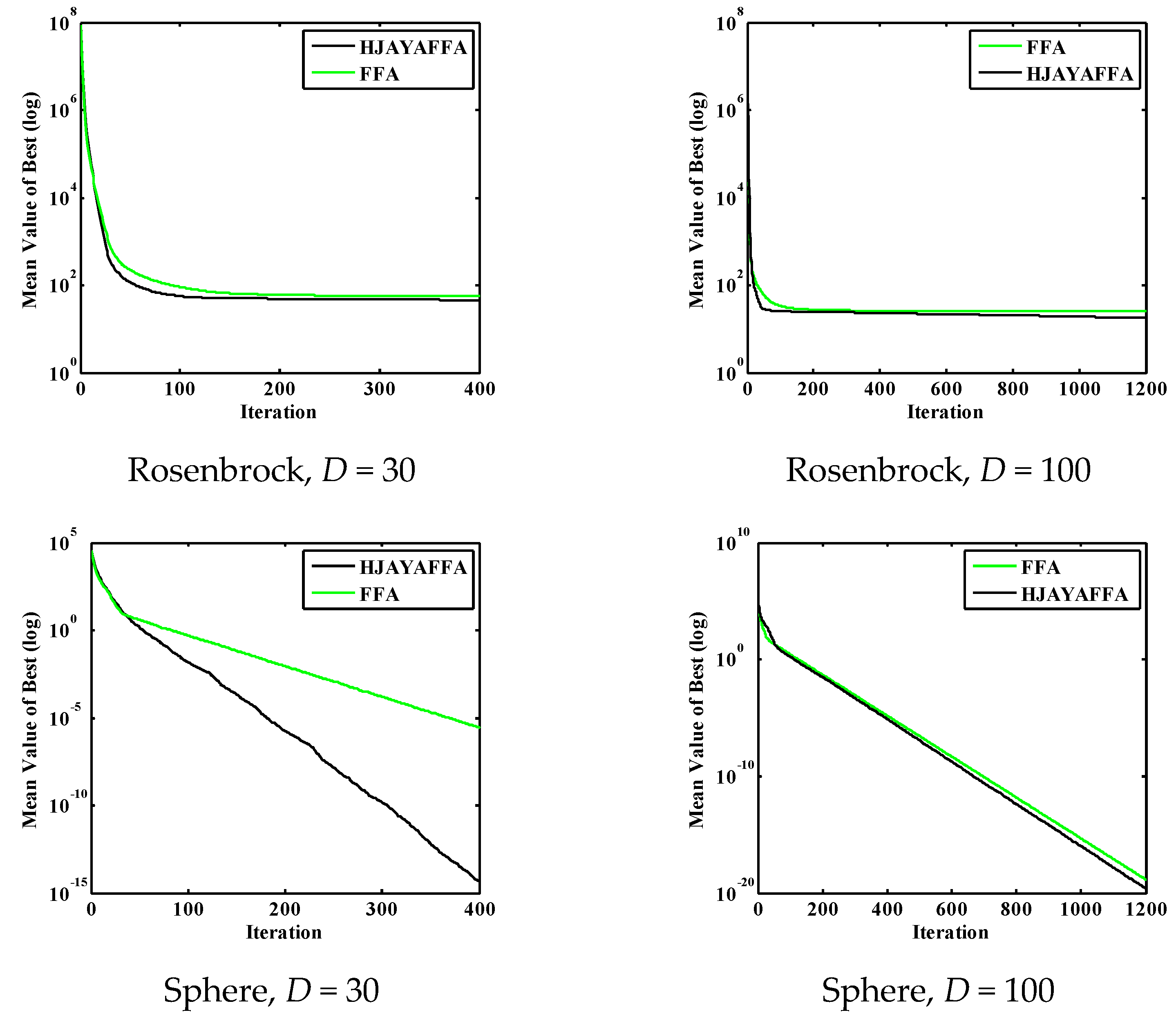
| Rosenbrock [−32, 32] | Unimodal | 56.7494 23.2999 81.0251 | 45.5246 0.1357 29.1884 | 26.3190 23.8039 10.8648 | 17.8910 15.8155 1.1293 |
| Sphere [−100, 100] | Unimodal | 2.7196×10⁻⁶ 1.9314×10⁻⁶ 3.5034×10⁻⁷ | 4.3637 × 10⁻¹⁵ 7.3028 × 10⁻¹⁷ 8.5226 × 10⁻¹⁵ | 1.4702×10⁻¹⁹ 1.3292×10⁻¹⁹ 8.1340×10⁻²¹ | 2.6643 × 10−;20 5.9287 × 10⁻²¹ 2.0183 × 10⁻²⁰ |
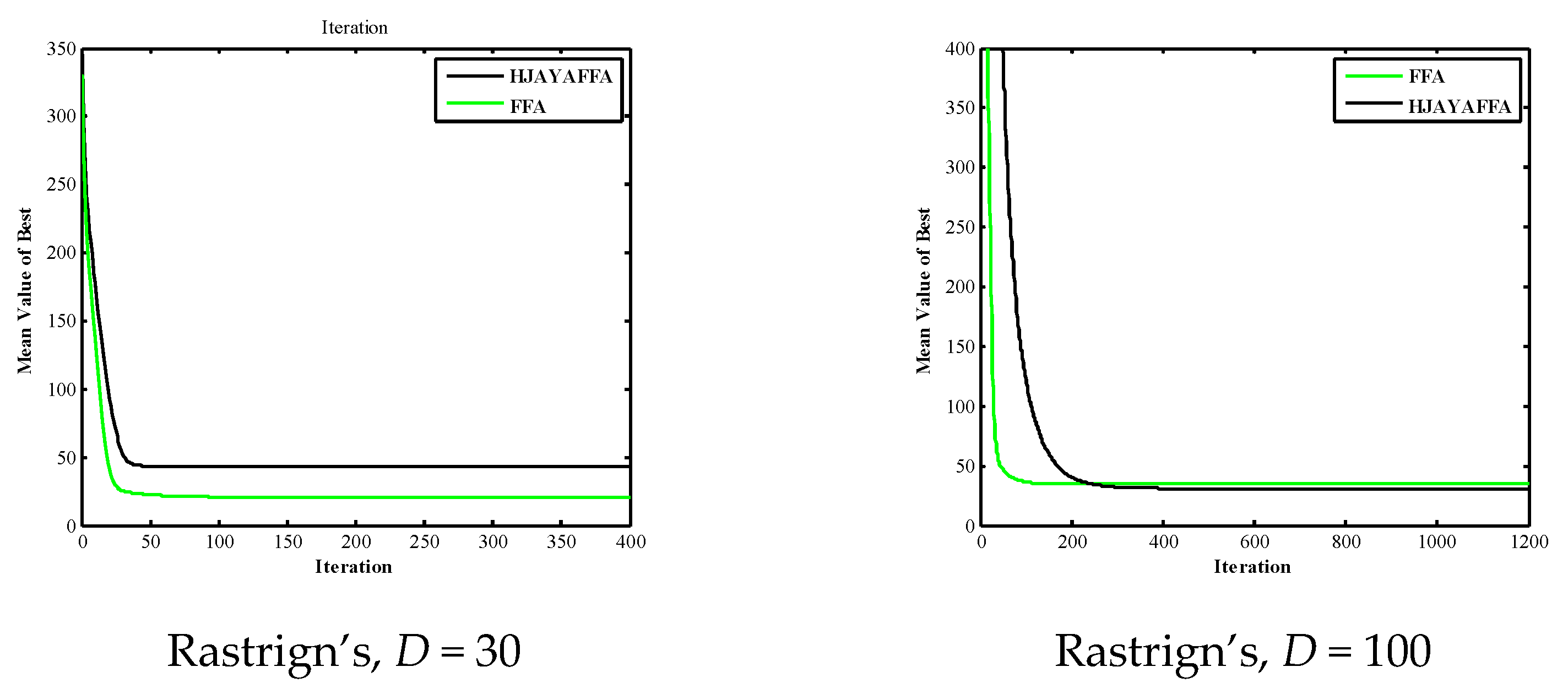
| Rastrign’s [−5.12, 512] | Multimodal | 20.5293 6.9647 6.0745 | 43.5562 4.7033 13.5772 | 34.9728 19.8992 11.8223 | 30.8437 17.8841 8.2046 |
| Variables Optimal Values | Limits | The Cases | ||||||
|---|---|---|---|---|---|---|---|---|
| Min | Max | 1 | 2 | 3 | 4 | 5 | 6 | |
| PG1 (MW) | 50 | 250 | 177.0297 | 139.9985 | 198.7328 | 102.6069 | 176.3325 | 126.7899 |
| PG2 (MW) | 20 | 80 | 48.7224 | 54.9972 | 44.8834 | 55.5590 | 48.8232 | 52.0824 |
| PG5 (MW) | 15 | 50 | 21.3825 | 24.1391 | 18.4734 | 38.1133 | 21.6338 | 30.2948 |
| PG8 (MW) | 10 | 35 | 21.2881 | 4.9826 | 10.0000 | 35.0000 | 22.2391 | 34.9995 |
| PG11 (MW) | 10 | 30 | 11.9890 | 18.6929 | 10.0001 | 30.0000 | 12.2210 | 25.0682 |
| PG13 (MW) | 12 | 40 | 12.0017 | 17.3272 | 12.0000 | 26.6501 | 12.0000 | 20.0045 |
| VG1 (p.u.) | 0.95 | 1.1 | 1.0836 | 1.0735 | 1.0816 | 1.0698 | 1.0423 | 1.0737 |
| VG2 (p.u.) | 0.95 | 1.1 | 1.0605 | 1.0565 | 1.0579 | 1.0576 | 1.0228 | 1.0574 |
| VG5 (p.u.) | 0.95 | 1.1 | 1.0337 | 1.0298 | 1.0302 | 1.0359 | 1.0145 | 1.0323 |
| VG8 (p.u.) | 0.95 | 1.1 | 1.0382 | 1.0405 | 1.0371 | 1.0438 | 1.0055 | 1.0406 |
| VG11 (p.u.) | 0.95 | 1.1 | 1.0991 | 1.0915 | 1.0995 | 1.0834 | 1.0733 | 1.0405 |
| VG13 (p.u.) | 0.95 | 1.1 | 1.0519 | 1.0650 | 1.0633 | 1.0573 | 0.9873 | 1.0242 |
| T6–9 (p.u.) | 0.9 | 1.1 | 1.0713 | 1.0616 | 1.0417 | 1.0653 | 1.0999 | 1.1000 |
| T6–10 (p.u.) | 0.9 | 1.1 | 0.9183 | 0.9112 | 0.9692 | 0.9205 | 0.9000 | 0.9503 |
| T4–12 (p.u.) | 0.9 | 1.1 | 0.9774 | 1.0028 | 0.9951 | 0.9901 | 0.9381 | 1.0334 |
| T28–27(p.u.) | 0.9 | 1.1 | 0.9743 | 0.9743 | 0.9776 | 0.9750 | 0.9710 | 1.0048 |
| QC10 (MVAR) | 0.0 | 5.0 | 2.6745 | 1.1882 | 4.7749 | 4.9569 | 4.9638 | 3.1583 |
| QC12 (MVAR) | 0.0 | 5.0 | 1.2842 | 1.2617 | 1.9178 | 0.1636 | 0.0080 | 0.0291 |
| QC15 (MVAR) | 0.0 | 5.0 | 4.2681 | 4.7107 | 3.7824 | 4.4512 | 5.0000 | 3.9138 |
| QC17 (MVAR) | 0.0 | 5.0 | 5.0000 | 4.2344 | 4.5810 | 5.0000 | 0 | 4.9986 |
| QC20 (MVAR) | 0.0 | 5.0 | 4.2732 | 4.2153 | 4.3853 | 4.2168 | 5.0000 | 4.9972 |
| QC21 (MVAR) | 0.0 | 5.0 | 4.9997 | 4.9164 | 4.9552 | 5.0000 | 5.0000 | 4.9994 |
| QC23 (MVAR) | 0.0 | 5.0 | 3.4064 | 3.0390 | 2.8829 | 3.2778 | 5.0000 | 4.3156 |
| QC24 (MVAR) | 0.0 | 5.0 | 4.9966 | 4.8430 | 4.9368 | 5.0000 | 5.0000 | 4.9969 |
| QC29 (MVAR) | 0.0 | 5.0 | 2.6155 | 2.5157 | 2.6963 | 2.5602 | 2.6384 | 2.6202 |
| Cost (USD/h) | - | - | 800.4800 | 646.5020 | 832.1798 | 859.0165 | 803.7036 | 825.0311 |
| Emission (t/h) | - | - | 0.3659 | 0.2835 | 0.4378 | 0.2289 | 0.3638 | 0.2597 |
| Power losses (MW) | - | - | 9.0134 | 6.7375 | 10.6897 | 4.5293 | 9.8496 | 5.8393 |
| V.D. (p.u.) | - | - | 0.9047 | 0.9041 | 0.8578 | 0.9327 | 0.0948 | 0.2956 |
| Optimizer | Fuel Cost (USD/h) | Emission (t/h) | Power Losses (MW) | V.D. (p.u.) |
|---|---|---|---|---|
| PSOGSA [58] | 800.49859 | - | 9.0339 | 0.12674 |
| JAYA [13] | 800.4794 | - | 9.06481 | 0.1273 |
| MSA [9] | 800.5099 | 0.36645 | 9.0345 | 0.90357 |
| ARCBBO [59] | 800.5159 | 0.3663 | 9.0255 | 0.8867 |
| FPA [9] | 802.7983 | 0.35959 | 9.5406 | 0.36788 |
| GWO [42] | 801.41 | - | 9.30 | - |
| IEP [60] | 802.46 | - | - | - |
| TS [16] | 802.29 | - | - | - |
| MICA-TLA [61] | 801.0488 | - | 9.1895 | - |
| MGBICA [62] | 801.1409 | 0.3296 | - | - |
| ABC [17] | 800.660 | 0.365141 | 9.0328 | 0.9209 |
| SFLA-SA [63] | 801.79 | - | - | - |
| MFO [9] | 800.6863 | 0.36849 | 9.1492 | 0.75768 |
| MHBMO [42] | 801.985 | - | 9.49 | - |
| AGSO [20] | 801.75 | 0.3703 | - | - |
| DE [64] | 802.39 | - | 9.466 | - |
| SKH [65] | 800.5141 | 0.3662 | 9.0282 | - |
| EP [66] | 803.57 | - | - | - |
| MPSO-SFLA [48] | 801.75 | - | 9.54 | - |
| FA | 800.7502 | 0.36532 | 9.0219 | 0.9205 |
| HFAJAYA | 800.4800 | 0.3659 | 9.0134 | 0.9047 |
| Optimizer | Fuel Cost (USD/h) | Emission (t/h) | Power Losses (MW) | V.D. (p.u.) |
|---|---|---|---|---|
| FA | 647.2612 | 0.2835 | 6.7302 | 0.8915 |
| HFAJAYA | 646.5020 | 0.2835 | 6.7375 | 0.9041 |
| LTLBO [18] | 647.4315 | 0.2835 | 6.9347 | 0.8896 |
| MSA [9] | 646.8364 | 0.28352 | 6.8001 | 0.84479 |
| MICA-TLA [61] | 647.1002 | - | 6.8945 | - |
| MPSO-SFLA [48] | 647.55 | - | - | - |
| MDE [64] | 647.846 | - | 7.095 | - |
| GABC [67] | 647.03 | - | 6.8160 | 0.8010 |
| FPA [9] | 651.3768 | 0.28083 | 7.2355 | 0.31259 |
| SSO [39] | 663.3518 | - | - | - |
| MFO [9] | 649.2727 | 0.28336 | 7.2293 | 0.47024 |
| IEP [60] | 649.312 | - | - | - |
| Optimizer | Fuel Cost (USD/h) | Emission (t/h) | Power Losses (MW) | V.D. (p.u.) |
|---|---|---|---|---|
| FA | 832.5596 | 0.4372 | 10.6823 | 0.8539 |
| HFAJAYA | 832.1798 | 0.4378 | 10.6897 | 0.8578 |
| SP-DE [57] | 832.4813 | 0.43651 | 10.6762 | 0.75042 |
| PSO [10] | 832.6871 | - | - | - |
| Optimizer | Fuel cost (USD/h) | Emission (t/h) | Power Losses (MW) | V.D. (p.u.) |
|---|---|---|---|---|
| FA | 859.8325 | 0.2289 | 4.5398 | 0.9330 |
| HFAJAYA | 859.0165 | 0.2289 | 4.5293 | 0.9327 |
| SF-DE [57] | 859.1458 | 0.2289 | 4.5245 | 0.92731 |
| MSA [9] | 859.1915 | 0.2289 | 4.5404 | 0.92852 |
| Optimizer | Fuel Cost (USD/h) | Emission (t/h) | Power Losses (MW) | V.D. (p.u.) |
|---|---|---|---|---|
| FA | 804.9733 | 0.3637 | 9.8837 | 0.0950 |
| HFAJAYA | 803.7036 | 0.3638 | 9.8496 | 0.0948 |
| MOMICA [68] | 804.9611 | 0.3552 | 9.8212 | 0.0952 |
| ECHT-DE [57] | 803.7198 | 0.36384 | 9.8414 | 0.09454 |
| BB-MOPSO [68] | 804.9639 | - | - | 0.1021 |
| MFO [9] | 803.7911 | 0.36355 | 9.8685 | 0.10563 |
| MNSGA-II [68] | 805.0076 | - | - | 0.0989 |
| MPSO [9] | 803.9787 | 0.3636 | 9.9242 | 0.1202 |
| Algorithm | Fuel Cost (USD/h) | Emission (t/h) | Power Losses (MW) | V.D. (p.u.) |
|---|---|---|---|---|
| FA | 828.1568 | 0.2602 | 5.9015 | 0.3137 |
| HFAJAYA | 825.0311 | 0.2597 | 5.8393 | 0.2956 |
| MOMICA [68] | 830.1884 | 0.2523 | 5.5851 | 0.2978 |
| MFO [9] | 830.9135 | 0.25231 | 5.5971 | 0.33164 |
| MNSGA-II [68] | 834.5616 | 0.2527 | 5.6606 | 0.4308 |
| MSA [9] | 830.639 | 0.25258 | 5.6219 | 0.29385 |
| BB-MOPSO [68] | 833.0345 | 0.2479 | 5.6504 | 0.3945 |
| Wind Power Generating Plants | Solar PV Plant | ||||||
|---|---|---|---|---|---|---|---|
| Wind Farm | No. of Turbines | Rated Power, Pwr (MW) | Weibull PDF parameters | Weibull Mean, Mwbl | Rated Power, Psr (MW) | Lognormal PDF parameters | Lognormal Mean, Mlgn |
| 1 (bus 5) | 25 | 75 | c = 9, k = 2 | v = 7.976 m/s | 50 (bus 13) | µ = 6, σ = 0.6 | G = 483 W/m2 |
| 2 (bus 11) | 20 | 60 | c = 10, k = 2 | v = 8.862 m/s | |||
| Variables | Optimal Values | |
|---|---|---|
| PG1 (MW) | 134.90791 | |
| PG2 (MW) | 28.7687 | |
| Pws1 (MW) | 43.8862 | |
| PG3 (MW) | 10 | |
| Pws2 (MW) | 37.049 | |
| Pss (MW) | 34.5606 | |
| VG1 (p.u.) | 1.0717 | |
| VG2 (p.u.) | 1.0568 | |
| VG5 (p.u.) | 1.0348 | |
| VG8 (p.u.) | 1.0547 | |
| VG11 (p.u.) | 1.0982 | |
| VG13 (p.u.) | 1.049 | |
| QG1 (MVAR) | −2.33741 | |
| QG2 (MVAR) | 11.7952 | |
| Qws1 (MVAR) | 22.4203 | |
| QG3(MVAR) | 40 | |
| Qws2 (MVAR) | 30 | |
| Qss (MVAR) | 15.1297 | |
| Fuelvlvcost (USD/h) | 441.4626 | |
| Wind gen cost (USD/h) | 247.0741 | |
| Solar gen cost (USD/h) | 93.7428 | |
| Total Cost (USD/h) | 782.2795 | |
| Emission (t/h) | 1.76202 | |
| Power losses (MW) | 5.7724 | |
| V.D. (p.u.) | 0.45423 |
| Variables | Optimal Values | |
|---|---|---|
| PG1 (MW) | 122.91239 | |
| PG2 (MW) | 31.4629 | |
| Pws1 (MW) | 45.1894 | |
| PG3 (MW) | 10 | |
| Pws2 (MW) | 38.0721 | |
| Pss (MW) | 41.0406 | |
| VG1 (p.u.) | 1.0701 | |
| VG2 (p.u.) | 1.0566 | |
| VG5 (p.u.) | 1.0354 | |
| VG8 (p.u.) | 1.0403 | |
| VG11 (p.u.) | 1.0999 | |
| VG13 (p.u.) | 1.0573 | |
| QG1 (MVAR) | −2.82122 | |
| QG2 (MVAR) | 12.1528 | |
| Qws1 (MVAR) | 22.9933 | |
| QG3(MVAR) | 35.0868 | |
| Qws2 (MVAR) | 30.0 | |
| Qss (MVAR) | 18.2947 | |
| Fuelvlvcost (USD/h) | 422.6759 | |
| Wind gen cost (USD/h) | 255.1889 | |
| Solar gen cost (USD/h) | 115.4701 | |
| Total Cost (USD/h) | 810.5517 | |
| Emission (t/h) | 0.86084 | |
| Power losses (MW) | 5.2775 | |
| V.D. (p.u.) | 0.47175 | |
| Carbon tax (USD/h) | 17.2168 |
| Optimizer | Min | Mean | Max | Std. | Time (s) |
| Case 1 | |||||
| HFAJAYA | 800.4800 | 800.5095 | 800.5378 | 0.0095 | 20.6 |
| FA | 800.7502 | 8001.0924 | 801.6420 | 1.82 | 20.6 |
| Optimizer | Min | Mean | Max | Std. | Time (s) |
| Case 2 | |||||
| HFAJAYA | 646.5020 | 646.6267 | 646.7001 | 0.017 | 20.7 |
| FA | 647.2612 | 647.5939 | 647.2614 | 0.823 | 20.7 |
| Optimizer | Min | Mean | Max | Std. | Time (s) |
| Case 3 | |||||
| HFAJAYA | 832.1798 | 832.3673 | 832.6049 | 0.0097 | 20.7 |
| FA | 832.5596 | 832.8512 | 833.1725 | 0.746 | 20.7 |
| Optimizer | Min | Mean | Max | Std. | Time (s) |
| Case 7 | |||||
| HFAJAYA | 782.2795 | 782.5472 | 782.7363 | 0.0648 | 21.4 |
| FA | 783.8409 | 784.6110 | 785.4923 | 1.84 | 21.5 |
Publisher’s Note: MDPI stays neutral with regard to jurisdictional claims in published maps and institutional affiliations. |
© 2022 by the author. Licensee MDPI, Basel, Switzerland. This article is an open access article distributed under the terms and conditions of the Creative Commons Attribution (CC BY) license (https://creativecommons.org/licenses/by/4.0/).
Share and Cite
Alghamdi, A.S. A Hybrid Firefly–JAYA Algorithm for the Optimal Power Flow Problem Considering Wind and Solar Power Generations. Appl. Sci. 2022, 12, 7193. https://doi.org/10.3390/app12147193
Alghamdi AS. A Hybrid Firefly–JAYA Algorithm for the Optimal Power Flow Problem Considering Wind and Solar Power Generations. Applied Sciences. 2022; 12(14):7193. https://doi.org/10.3390/app12147193
Chicago/Turabian StyleAlghamdi, Ali S. 2022. "A Hybrid Firefly–JAYA Algorithm for the Optimal Power Flow Problem Considering Wind and Solar Power Generations" Applied Sciences 12, no. 14: 7193. https://doi.org/10.3390/app12147193
APA StyleAlghamdi, A. S. (2022). A Hybrid Firefly–JAYA Algorithm for the Optimal Power Flow Problem Considering Wind and Solar Power Generations. Applied Sciences, 12(14), 7193. https://doi.org/10.3390/app12147193