The Optimal and Economic Planning of a Power System Based on the Microgrid Concept with a Modified Seagull Optimization Algorithm Integrating Renewable Resources

Abstract

In the past, planning to develop an electricity generation capacity supply of consumable load, an acceptable level of reliability, and minimum cost has played significant roles. Due to technological development in energy and the support of energy policymakers to make the most of these clean and cheap resources, a significant amount of research has been conducted to make the most of such energy. Constraints such as low capacity, output power uncertainty, and sustainability problems have made using distributed energy sources costly and complex. Theoretically, capacity development planning in a power system is part of macro-energy planning. It is generally based on specific development policies in each country’s national interest. In addition to being economical, the purpose of this planning was to find the best capacity development plan commensurate with the amount of consumption so that the development plan does not go beyond the permissible limits of reliability, environmental issues, and other constraints. On the other hand, due to the considerable growth of divided production, especially energy sources, it is essential to use microgrids. Accordingly, in this research study, in the process of solving the problem of planning and providing load growth by the distributed generation units to maximize reliability and minimize investment costs, the creation of smaller networks was investigated. To optimize zoning, the weighted graph theory method, in which the weight of the edges is the apparent power passing through the lines, was adopted. In addition, reactive power reliability was included in the calculations to improve the economic aspects. Probabilistic modeling for the presence of renewable resources was employed to bring the model to reality. Since the above problem is very complex, a Seagull-based algorithm and chaos theory were utilized to solve this matter. Finally, the suggested method for the sample system is discussed in different scenarios, indicating an improvement in the system’s performance. According to the numerical results, the NSGA, SPEA, and MOPSO have mean values of 68.3%, 50.2%, and 48.3%, which are covered by the proposed optimization algorithm.

1. Introduction

1.1. Aims and Difficulties

With the advancement of technology and the introduction of optimal economic issues in the processes and activities of the power network, new concepts have emerged in the power system. The spread of these new concepts, such as smart microgrids and active networks, has led to fundamental changes in the usual methods of planning and operating the power system. At the same time, the existing electricity network must be exploited optimally. The status of this network for the next few years should be considered [1,2,3]. If the existing production system in the power network cannot meet the consumer’s requirement, it is essential to add new production units. In recent years, the installation of distributed generation units (DGs) in the power grid has increased. These units generally have much less output (from a few kilowatts to several megawatts) and much smaller dimensions compared to the conventional concentrated power plants in the grid. The installation of these production units in the distribution network will have different effects on the network, both at the distribution level and at high levels.

In many cases, these resources are considered serious competitors to other network equipment. The study of the effects of DG installation on the power grid, of course, taking into account the existence of uncertainties in the parameters and input data, can help network operators and planners better manage the network’s development. Including substations and scattered products) and selecting the optimal installation location to meet the required load demand under the constraints of substation capacity, line heat capacity, voltage drop, radial network arrangement, and reliability are many variables that need to be considered. This optimization issue can be a crushing problem in a large-scale and complex combination [4,5].

1.2. Literature Review

Several articles have been presented in these fields [6,7,8,9]. In general, traditional methods refer to models used before discussing the electricity market and the economic justification of each project. New methods are called models that consider the impact of creating a competitive environment in the power system. Additionally, they try to upgrade the network according to the economic criteria of each project. The issue of production investing in both traditional and competitive environments has its own characteristics. In the traditional environment, characteristics including centralized decisions, price stability, access to complete information, and low uncertainty can be mentioned. However, in the new methods, in the form of a competitive environment, there are characteristics such as decentralized decision making, different prices, limited access to information, and high uncertainty [9]. In [10], a dynamic model is proposed to plan the development of distribution networks. In this model, to disturb the system to be responsive to load growth, DG integration with post-development (installation of new transformers) and modernization of feeders are considered, and these methods are compared. Investment, maintenance, operating, and loss costs are the goals of optimization, and optimal load distribution (OPF) was used to minimize them [11]. To reduce losses and increase the system’s reliability, the proposed DG values for a node are considered instead of comparing the load value of that node with the sum of loads of several nodes when disconnected from the network. The faces of the island are compared so that this action optimizes the value obtained. In [12], scattered production sources are also used to reduce the share of losses in addition to capacitors. First, the optimal locations of these sources are determined using voltage index analysis, and the amount of these sources is obtained using the proposed algorithm. In recent years, the focus on a concept, microgrids, has increased. Microgrid planning aimed to determine the output power of energy units is scattered; however, renewable sources’ uncertainty makes this planning difficult. In [13], the problem of the optimal utilization of microgrids has been solved by focusing on energy storage. However, it does not examine the fluctuations of renewable units. In [14], a new method based on optimal power flow in a wind farm is presented. Researchers in [15] presented a method in which the total cost of power generation in a micro-wind grid is optimized by considering its environmental variables. In [16], planning the production of distributed energy sources in the microgrid, with the aim of providing the required energy for electrical and thermal loads, is completed with the lowest possible cost and pollution in compliance with operating rules. In this work, a two-step solution for planning the economical production of microgrids is presented. Uncertainty modeling of wind and solar power generation is completed using the point estimation method. The results are sent to the second stage. The second stage is the program of optimal production of distributed microgrid energy resources to reduce the cost of environmental pollution by using an evolutionary algorithm. Additionally, some authorities have used possible planning methods and solved them in different ways. Researchers in [17] presented a possible method for managing energy in the microgrid, which also includes producing renewable resources. The problem of mixed linear programming with integers was solved by Bandar analysis. Researchers in [18] suggested a possible microgrid energy planning in which different distributed generation technologies, renewable resources, and storage are considered. In this study, the problem of possible planning was solved with the help of intelligent methods. Researchers in [19] assessed the problem of bringing production units into orbit, taking into account the uncertainty of wind and solar and load consumption, which are intended to be optimized, and reduce costs and pollution. In this study, several valid scenarios for the uncertainty of wind, solar, and load sources are considered. Under different scenarios, an algorithm for cost and pollution minimization (their mathematical hope) is presented. In [20], an optimal method for designing multiple microgrids is considered, which examines the reliability and security of the distribution system to collect the distribution network for microgrids considering network reliability. Researchers in [21] proposed a multi-objective economic method considering the probabilistic nature of distributed renewable generation resources to design a single microgrid. The design of microgrids based on self-healing against possible accidents in the distribution network was investigated in [22]. In this reference, network partitioning was evaluated with the aim of studying the least loading of the system. The purpose [23] of zoning distribution networks was to improve the reliability of the entire system. Researchers in [24] is suggested an optimal method for producing distributed renewable sources. The design of microgrids using graph theories was proposed in [25]. In this paper, the structure design of microgrids using graph partitioning theory as a circular structure with system reliability was investigated.

1.3. Novelties and Motivations

Reviewing the published articles in this field, it can be concluded that the structuring of the power system based on the microgrid model has not been completed simultaneously for the economic base and the qualities of reliability. Additionally, in probabilistic model research, wind and solar sources as a source with uncertainty have not been determined. In addition, solving the above problem by considering cases related to these principles will be very complex. Using the methods used in the articles cannot guarantee an optimal answer. Therefore, there is a current need to present an optimization algorithm that will be more efficient. After reviewing the mentioned works, the use of solar radiation causes the forecast of production of these sources to be accompanied by uncertainty. For example, in planning for the next day, it is impossible to precisely determine the amount of renewable energy production. Forecasting the future is filled with mistakes, which challenges energy planning. Since most distribution systems are now traditional networks fed by the global network, their transformation into smaller networks in the presence of distributed generation sources with probabilistic, non-probabilistic production and reactive power supply requires new design methods. Given that scattered products are an integral part of microgrids, planning and exploiting these resources in new networks requires a new design. In addition, published articles use methods that are not guaranteed to find the optimal answer. It is possible to be in local points by increasing the number of constraints and decision variables. Here, the graph theory model is used to create microgrids to cover these cases. The zoning step to create microgrids in the distribution network is associated with a planning problem. To more accurately model the problem of distributed generation with probabilistic nature and loads on an hourly basis, all costs and complete indicators to consider power for the reliability of microgrids are also considered. Accordingly, the main essential novelties and highlights of this paper are summarized as follows:

• Employed the reliability indices in optimal and secure reactive power planning.
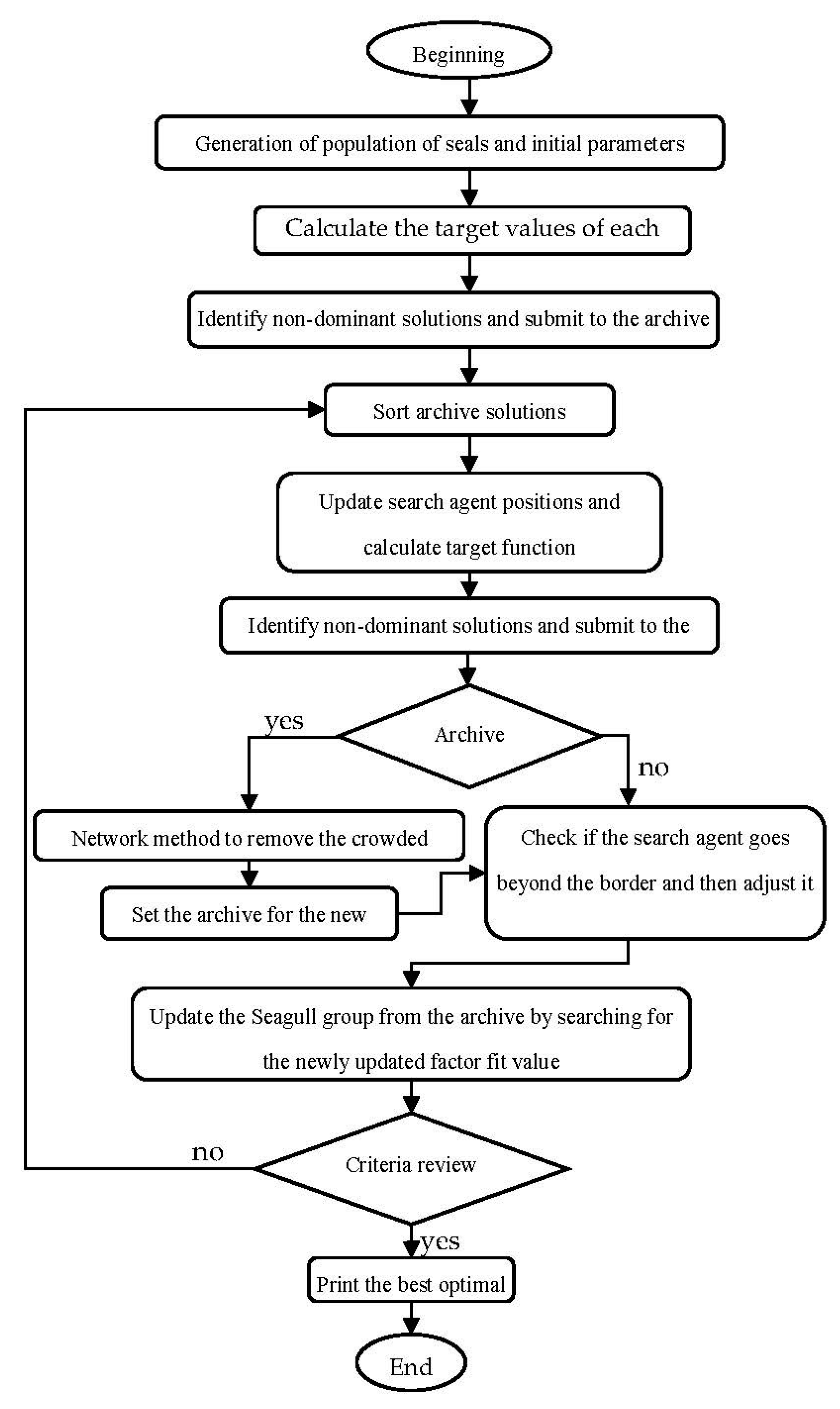
• Proposed a modified version of the Seagull optimization algorithm.
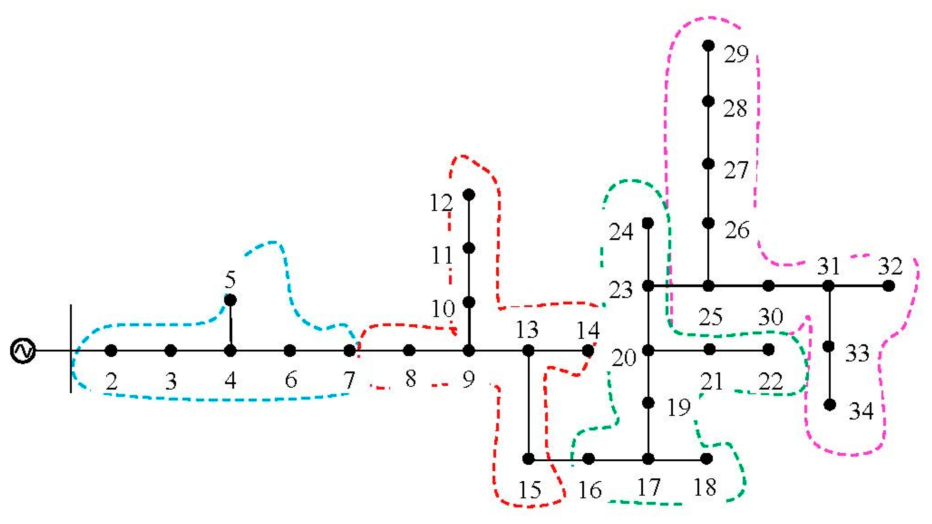
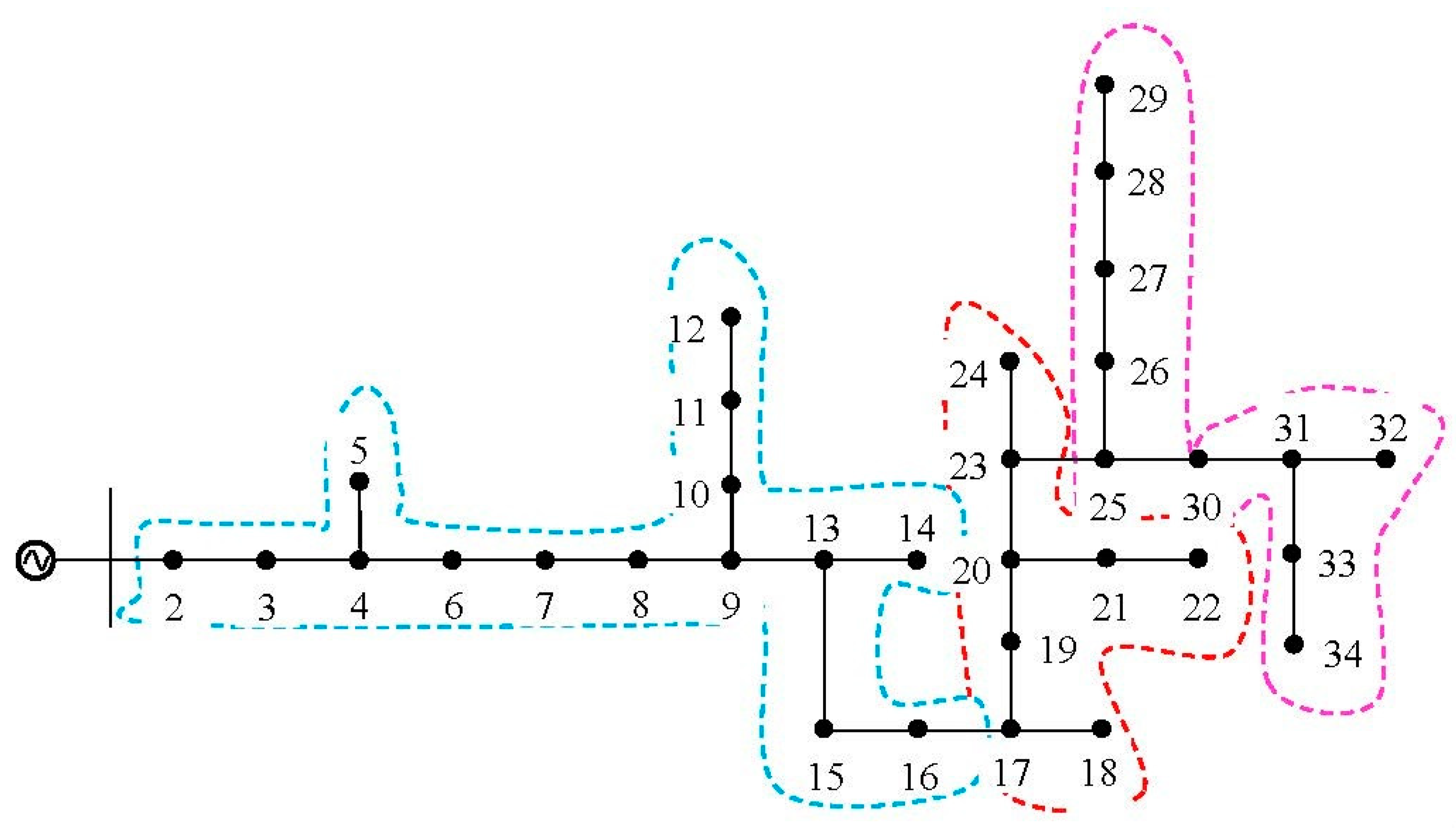
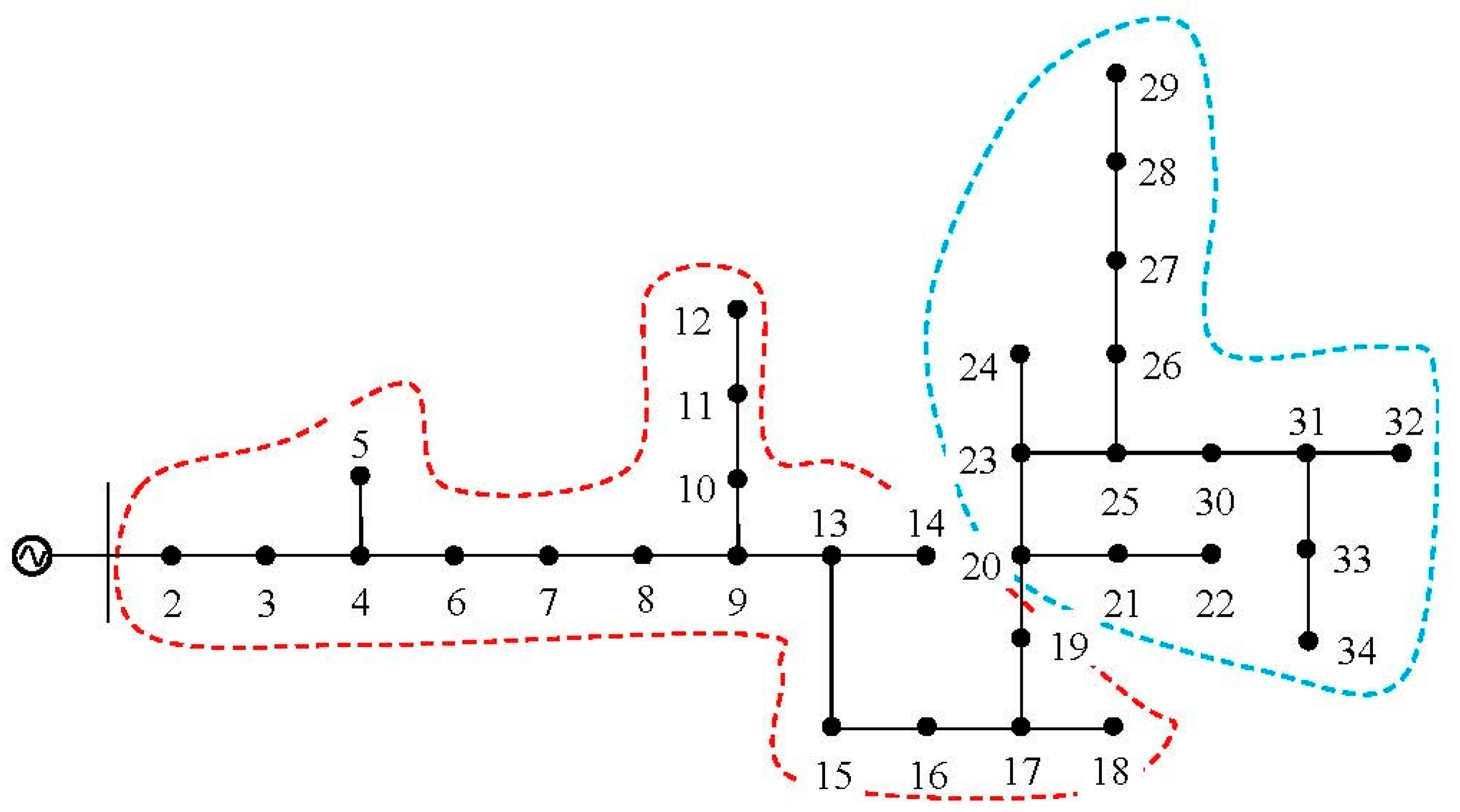
• Used the graph method to determine the boundaries of microgrids and evaluate its capacity in the power system.
• Investigated microgrid performance in various operating conditions.
• Considered the probabilistic and uncertainty items of renewable resources.

1.4. Paper Layout

The rest of the article is organized as follows: the system modeling and related mathematics of objective functions and constraints are presented. Additionally, an optimization algorithm is suggested to solve the matter, and the results of the simulations and numerical and comparative analyses are presented and discussed.

2. Modeling the Problem under Study

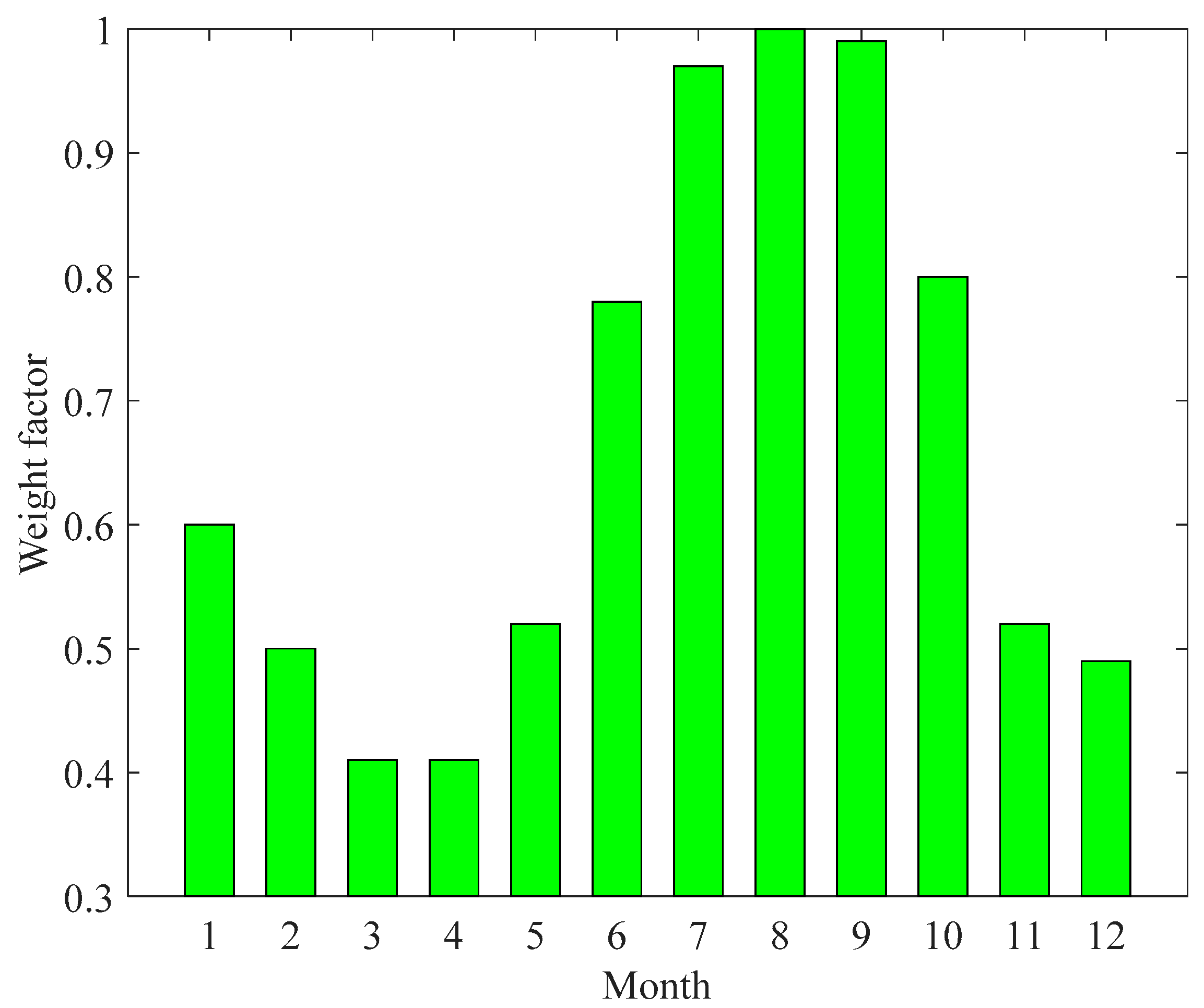
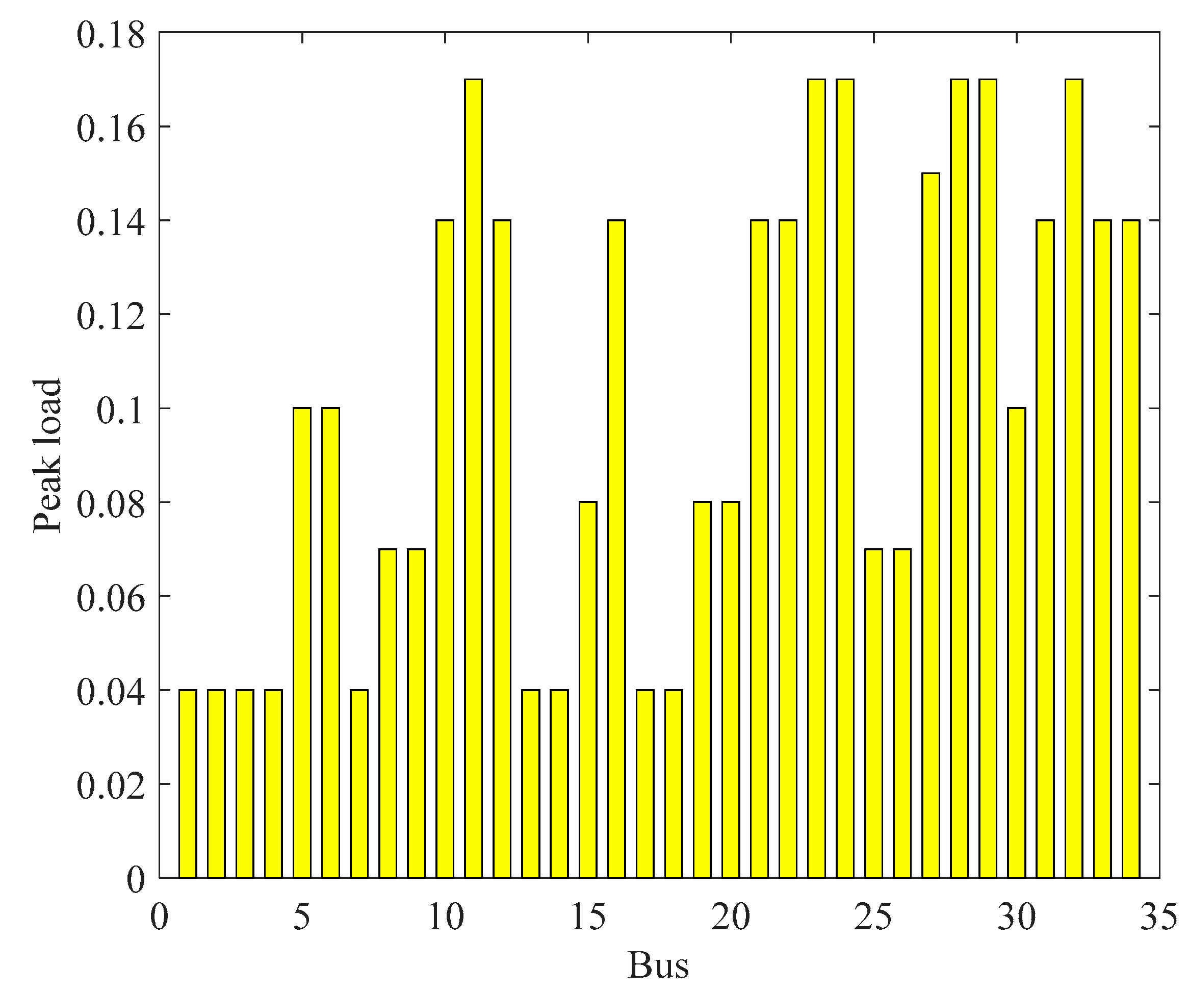
In this section, the necessary relations and explanations for modeling the studied problem are presented.

2.1. Load Modeling

Climatic positions are affected by the system, and many of these events are repetitive. They happen for a year. Load models of different times can be obtained by using historical data. In this study, information is modeled in Figure 1, Figure 2 and Figure 3. Equation (1) is predicted at another time [4].

$$L_i(t)=w(h)\times w(m)\times L_p(i)$$

(1)

Due to the demand for high-quality and reliable electricity, one of the critical factors is the necessary readiness to supply the energy required by consumers in the operation of the network. For this purpose, in predicting network conditions for planning and utilization of available resources, due to the possibility of error, values are measured and sampled in the past, and the resulting answers have some uncertainty. However, the most critical error in these predicted values is not considering the uncertainty that exists in predicting the future of the network. Therefore, the distribution network operator can achieve a more efficient network operation by considering the uncertainty in these variables. If y = f(Z) is a multi-objective function, and Z is described as an indefinite vector with a corresponding density function. In this method, different scenarios are calculated according to the probability density function (PDF) associated with each uncertain variable of production Z_s and the value of y as follows:

$$y={\displaystyle \sum _{s\in {\mathsf{\Omega }}_s}{\pi }_s\times f\left(Z_s\right)}$$

(2)

The ${\mathsf{\Omega }}_s$ state probability is the sum of all the states considered for the uncertain parameter $Z$. If there are several variables with different scenarios, the ${\pi }_s$ probability related to the $s$ condition is calculated as follows:

$${\pi }_s={\displaystyle \prod _{x\in \gamma }{\pi }_x}\hspace{1em}\hspace{1em}\forall s\in {\mathsf{\Omega }}_s$$

(3)

The ${\pi }_x$ probability of an uncertain parameter $x$ and $\gamma$ is the set of uncertain parameters.

2.2. Production of Wind Turbine

The Weibal distribution function is considered to model wind speed due to its high accuracy in describing the probable wind speed [26]:

$$f\left(x|\lambda ,k\right)=\frac{k}{\lambda }{\left(\frac{\lambda }{x}\right)}^{k-1}{e}^{-{\left(\frac{x}{\lambda }\right)}^k}$$

(4)

where $k$ is the shape parameter and the $\lambda$ is the scale parameter. The following linear estimation equation is used to obtain the wind power distribution and shown in Figure 4:

$$\mathsf{\Omega }=\{\begin{array}{ll}0\hfill & ifX\le V_{ci}orX>V_{co}\hfill \\ \alpha +\beta X\hfill & if{V}_{ci}\le X\le V_r\hfill \\ M\hfill & if{V}_r\le X\le V_{co}\hfill \end{array}$$

(5)

where $\mathsf{\Omega }$ indicates the injected power by the wind power. The $X$ actual wind speed shows the maximum wind turbine output power, the linear coefficients of the equation, the normal wind speed, and the maximum and minimum wind speed for which power is not generated. The trend of wind speed and power is the same.

2.3. Photovoltaic System

To show the random PV production and energy demand, the normal distribution function with knowledge of the mean value and variance shown in Figure 5 is considered. The description of the normal distribution function is as follows:

$$f\left(x|m,{\vartheta }^2\right)=\frac{1}{\sqrt{2\pi }\vartheta }\exp \left(-\frac{{\left(x-m\right)}^2}{2{\vartheta }^2}\right)\hspace{1em}-\infty <x<\infty$$

(6)

The $m$ means the input variable ${\vartheta }^2$ is variance. The probability density function diagram is subdivided into the number of different probability levels according to the required accuracy to implement the model based on the scenario. In the normal distribution, the probability of each scenario and its mean are obtained based on Equations (7) and (8).

$${\pi }_{\rho }={\displaystyle \underset{S_i}{\oint }f\left(x|m,{\vartheta }^2\right)dx}$$

(7)

$$p{\rho }_s={\displaystyle \underset{S_i}{\oint }xf\left(x|m,{\vartheta }^2\right)dx}$$

(8)

The ${\pi }_{\rho }$ is probability of $S$ occurrence of my PV generation $p{\rho }_s$ scenario is the average in each of the PV scenarios. According to Figure 5, scenarios for constructing the final set of scenarios according to Equation (2) are combined as follows [27]:

$${\pi }_s={\pi }_w\times {\pi }_{\rho }\times {\pi }_l$$

(9)

where ${\pi }_w$, ${\pi }_{\rho }$, and ${\pi }_l$ in turn, show the probability scenarios of $w$ the wind farm, $\rho$ solar power plant, and $l$ load. The sum of the number of scenarios is obtained from the $w_n\times {\rho }_n\times l_n$ relation, in which $w_n,{\rho }_n,l_n$ are the number of states considered for load, PV, and wind, respectively.

2.4. Grid Zoning by Graph Method

Due to advances in electricity generation and the increasing use of distributed generation (DG) in distribution systems, it is necessary to convert existing distribution networks into smaller networks (microgrids) or a set of networks to improve the efficiency of systems. It is small so that it can be operated independently. The graph method described below is used to achieve the mentioned goals resulting from dividing and converting a traditional distribution network into microgrids containing scattered products. Recent advances in mathematics, especially in its applications, have led to the dramatic development of graph theory, with graph theory now being used for research in various fields, such as electrical networks, coding, computer science, and chemistry. Given the differences in goals in the optimization problem, the result will not be the only answer. Different solutions, each successful in several optimized functions, can be considered as optimal. One of the advantages of the optimization algorithm with several functions is to provide a set of optimal answers.

There is a problem in zoning a graph $G=(V,e)$ that includes n vertices. The edges of a graph may also be weighted, called a weighted graph. The concept of a weighted graph, in which each edge is assigned a number as its weight, has been used in many applications by the matrix W, which resembles the neighborhood matrix A with dimensions n × n, is stated [4]:

$$A=[{\alpha }_{ij}]\hspace{1em}\hspace{1em}i=1,\dots ,n\hspace{1em}j=1,\dots ,n$$

(10)

If there is an edge between vertices, i and j then ${\alpha }_{ij}=1$; otherwise, ${\alpha }_{ij}=0$. To form the matrix W, the same procedure is performed as for the neighborhood matrix A, with the difference that instead of a numeric one, the weight of that edge is placed:

$$W=[w_{ij}]\hspace{1em}\hspace{1em}i=1,\dots ,n\hspace{1em}j=1,\dots ,n$$

(11)

If the edge is between the vertices, then $w_{ij}=weight\mathrm{of}\mathrm{edge}\mathrm{between}ij$ and otherwise $w_{ij}=0$. A weighted graph was used to model the distribution network with all the conditions of a graph. For zoning this graph and more accurate simulation of the weight distribution system of each edge, the apparent power of the lines is obtained from the load distribution program. After forming this graph and obtaining the corresponding matrix, several other graphs are needed to solve the zoning problem, which are defined as follows. The degree gradient matrix is defined in such a way that all non-original diameter arrays are zero, and the original diameter arrays are obtained from the sum of the arrays of each row of the matrix [4]:

$$D=[dj]\hspace{1em}\hspace{1em}i=1,\dots ,n\hspace{1em}j=1,\dots ,n$$

(12)

If the edge is between vertices i and j, then $d_{ij}={\displaystyle {\sum }_{k=1}^n{w}_{ik}},i=j$; otherwise, $d=0,i\ne j$. The row sum of this matrix is equal to zero, so it has a specific value of zero. On the other hand, because the positive matrix is semi-definite, their other eigenvalues are absolute values. This matrix contains essential information from the graph configuration used here for zoning [28]. The problem is finding an area of vertex sets $P=\{P_1,\dots ,P_K\}$ based on the weight of the edges. Zoning based on the extraction spectrum or the same values and special vectors of the matrix corresponding to the system graph is provided to all the areas simultaneously by using the information in the special vector. After sorting the eigenvalues in ascending order $k,{\lambda }_1,\dots ,{\lambda }_k$, the eigenvalues $x_1,\dots ,x_k$ are smaller, and the eigenvectors correspond to these eigenvalues. By putting these special vectors together, a vector with dimensions is obtained that is used to form the zoning matrix as follows:

$$P=ZX{X}^{T}Z$$

(13)

where Z is a diagonal matrix with the following components and $x_{ih}^2$ matrix X components:

$$z_{ij}=\frac{1}{\sqrt{{\displaystyle {\sum }_{h=1}^k{x}_{ih}^2}}}$$

(14)

The material of the matrix $P_{ij}$ in relation (6) is the cosine of the angle between two rows of i and j vectors and indicates the proximity of the vertices to each other. The first vertex is randomly selected, and it can be considered as the boundary of the first region (for example, the $C1$ vertex). To find the second vertex, the minimum value $P_{ic1}$ is calculated per $i=1,\dots ,n$. The following equation is used to find the boundaries of other regions [4]:

$$Min\mathrm{Y}=P_{ic1}+P_{ic2}+\dots +P_{ick}$$

(15)

In general, in a weighted graph, the regions are selected according to the correlation between them, which is due to the use of special values and the Laplacian matrix of the graph. To select areas using the graph method, first, a bus is considered as the boundary of the first area, and other areas are obtained by using the matrix (proximity matrix) relative to that bus. Now, by changing the first selected bus in the first area, the corresponding bus in the matrix is changed from a close point of view, and the boundaries of other areas will also change relative to it. In addition, according to the network topology for each system, the number of areas does not exceed a certain value obtained in the simulation. As the network is limited, changing the bus does not achieve any number of divisions at first.

2.5. Assessing Reliability and Proposed Indicators

Based on the purpose of this work, which is to improve the reactive power of the network in the planning stage, first, the effect of reactive power on a reliability parameter is investigated. Then, four reliability indicators, including unsecured energy and unsecured clock, were combined to form a single index due to a lack of active and reactive power. Providing reactive power locally in a power system causes the reactive power component of the current passing through the lines to be relatively compensated. Consequently, the current size is reduced. Reducing the current size will reduce the active and reactive power losses proportional to the square of the current and the feeder temperature. According to [4], the expected life of insulation materials decreases exponentially with an increasing temperature. As a result, the feeder failure rate will decrease after the optimal placement of reactive power sources, and the distribution network reliability level will increase. Here, the branch has a component $(I{b}^r=I{b}^{0,r})$ and $\lambda b^0$ is an error rate. After compensation, the reactive current component of this branch will be zero, and the error rate $\lambda b^f$ will be changed. The mathematical modeling is as follows [4]:

$$\{\begin{array}{l}{I}_b^r=I_b^{0,r}\Rightarrow {\lambda }_b={\lambda }_b^0\\ I_b^r=0\Rightarrow {\lambda }_b={\lambda }_b^f\end{array}\forall b\in Sb\hspace{1em}Sb=\left\{1,\dots ,Nomber\mathit{of}\mathit{branches}\right\}$$

(16)

To evaluate the effect of compensating the reactive power component of the current on the failure rate, four mathematical functions, including linear, power, exponential, and logarithmic functions, can be considered. Fixed values of these functions $(A,B)$ are obtained by using test results. In this study, it is hypothesized that complete compensation of the reactive power component of the current reduces the feeder failure rate by a maximum of 28% [29]. The normalized feeder failure rate curves versus the normalized value of the reactive power component of the current are demonstrated in Figure 6.

Here, the linear function is used to model the error rate, while other functions are readily applicable to the problem. After modeling the effect of reactive power on the initial index (failure rate) and reliability for active and reactive power planning, we need to examine some additional indicators. For this purpose, the energy supply indicators and the hour supply due to a lack of active power and reactive are used as follows [30]:

$$EN{S}_P={\displaystyle {\sum }_{i=1}^{nc}L{C}_{P(i)}·{\lambda }_i}$$

(17)

$$EN{S}_Q={\displaystyle {\sum }_{i=1}^{nc}L{C}_{Q(i)}}·{\lambda }_i$$

(18)

$$VN{S}_P={\displaystyle {\sum }_{i=1}^{nc}Q{C}_{P(i)}·{\lambda }_i}$$

(19)

$$VN{S}_Q={\displaystyle {\sum }_{i=1}^{nc}Q{C}_{Q(i)}·{\lambda }_i}$$

(20)

In the above relations, ${\lambda }_i$ is the annual unavailability of the i load point, nc is events, $Q{C}_{p(i)},L{C}_{p(i)}$ is the amount of active and reactive load not applied, $Q{C}_{Q(i)},L{C}_{Q(i)}$ is the amount of active and reactive load not applied, $EN{S}_p$ and $EN{S}_Q$ are the energy applied due to a lack of active power, $VN{S}_p$ and $VN{S}_Q$ are reactive, and VAR represents unsecured clocks caused by a lack of active and reactive power.

2.6. Micro-Network Performance

For a distribution system consisting of several microgrids with distributed generation sources, it is necessary to recalculate the index of unsupplied energy. A microgrid was utilized to assess the reliability indicators. With such a design, in the event of an error in the microgrid, the exact part is turned off and separated from the rest of the system. This error causes the downstream microgrid to shut down unless there is enough scattered generation in other microgrids to supply loads. In the design phase, to minimize blackouts, the microgrid’s unsupplied energy, which is equal to the base value plus the unsupplied amount of energy, results from a mismatch between load and output. In other words, in addition to the amount of unsecured power of the microgrid, a positive number is added as a penalty coefficient. Therefore, the unsupplied energy and the amount and hour of unsupplied power for the microgrid can be calculated as follows [4]:

$$EN{S}_{p\_MG}=EN{S}_{P\_MG}{|}_{self}+(1-p_{MG})\times {\displaystyle \sum _{i=1}^{us}EN{S}_{Pi}}$$

(21)

$$EN{S}_{Q\_MG}=EN{S}_{Q\_MG}{|}_{self}+(1-p_{MG})\times {\displaystyle \sum _{i=1}^{us}EN{S}_{Qi}}$$

(22)

$$EV{S}_{P\_MG}=EV{S}_{P\_MG}{|}_{self}+(1-p_{MG})\times {\displaystyle \sum _{i=1}^{us}EV{S}_{Pi}}$$

(23)

$$EV{S}_{Q\_MG}=EV{S}_{Q\_MG}{|}_{self}+(1-p_{MG})\times {\displaystyle \sum _{i=1}^{us}EV{S}_{Qi}}$$

(24)

The subtitle represents the microgrid index, $p_{mg}$ probability number is the part of the year in which the output of the microgrid is more than the load, and it is calculated by using the probability states of the output-load. The general process of assessing reliability includes the following steps:

Step 1: Enter network information and its components, such as reliability data $EN{S}_p$ and $VN{S}_p$ network parameters.

Step 2: Calculate the amount of local compensated reactive power and the new value of feeder failure rate.

Step 3: If $Pi$ is bigger than $Pdi$, the algorithm goes to the next step; otherwise, the difference between the output and loads is calculated, updated, and completed.

Step 4: If $Qi$ is greater than $Qdi$, the algorithm goes to the next step; otherwise, the difference between the output and the proportional active and reactive load in all buses is calculated, updated, and completed.

Step 5: Calculate system reliability indicators.

Step 6: The planning problem compensates for the lack of active and reactive power by choosing the location and type of scattered products until the indicators reach their minimum value.

Step 7: If all the conditions are considered, the algorithm transfer to another step; otherwise, it transfers to 3 for the next state.

Step 8: Print the results.

2.7. Problem Objective Function

To solve the problem of planning, different objective functions or a combination of several objective functions can be considered multi-objective. There are three objective functions in optimization, which are:

(A)

Costs.

(B)

Reduce system line losses.

(C)

Reliability indicators.

All system development costs are included in two terms, the fixed costs (the construction of new units of distributed generation and reactive power sources and the cost of updating new feeders) and variable costs (the cost of maintenance and operation of the system, which is basically this cost). Existing posts are power supplies that can power at a given variable price ceiling. The cost function is described by [4]:

$$\mathrm{Cos}{t}_{total}=C_{FC}+C_{WT}+C_{PV}+C_{MS}+C_Q$$

(25)

Support is common in many parts of the world. The cost of a fuel cell is equal to [31]:

$$C_{FC.i}=0.04\times kW{h}^{-1}\times \frac{P_{FC,i}}{{\eta }_i}$$

(26)

$$PL{R}_i=\frac{P_{g,i}}{P_{\max ,i}}$$

(27)

$$\{\begin{array}{ll}if& PL{R}_i<0.05\Rightarrow {\eta }_i=0.2716\\ if& {\mathit{PLR}}_i\ge 0.05\Rightarrow {\eta }_i=0.2716PL{R}_i^5-2.9996PL{R}_i^4+3.6503PL{R}_i^3-2.0704PL{R}_i^2+0.3747\end{array}$$

(28)

The technology of using wind and solar to generate electricity is the new fastest-growing source of electricity supply globally. Wind energy is mainly generated by huge three-bladed wind turbines mounted on top of tall turrets, which work like reverse fans. Instead of using electricity to generate wind, these turbines utilize the wind to generate electricity. The resulting savings primarily preserve fossil energy resources and, more importantly, convert them into large amounts of high value-added petrochemicals. Secondly, the production of electricity from this type of energy is free of any environmental pollution, which contributes significantly to preserving the healthy nature of the human environment and thus provides a path to sustainable economic and social development. The following relations can express the cost function for wind and solar systems:

$$C_{PV,i}=a+b\times P_{PV,i}$$

(29)

$$C_{WT,i}=a+b\times P_{WT,i}$$

(30)

where $a=\frac{C_{Cap}(k{W}^{-1})\times Cap(kW)\times Gr}{Lif{e}_{time}(Year)\times 365\times 24\times LF}$ and $b=C_F(k{W}^{-1})+C_{O\&M}(k{W}^{-1})$ are involved in this relationship. The cost of power purchased from the main network is equal to [4]:

$$C_{MS}=price.P_{MC}$$

(31)

In recent years, the electricity industry in some countries of the world has become a competitive energy market in various ways, referred to as the restructured electricity industry. In the restructured electricity industry, the transmission system is a means of access for electricity sellers and buyers, which is unique and remains in the hands of the government. Its operation is left to the independent system operator. In such systems, where the production, transmission, distribution, and sale of electricity are made by different organs and companies, the accurate pricing of power or energy has a special feature and complexity. To transfer power with suitable and safe reliability from the point of the system (vendor), one of the most important services is the reactive power supply service in the system, without which it is not possible to transfer real power in the power system. For various reasons, such as novelty and complexity, the issue of reactive power service pricing in the restructured electricity industry has received less attention. The cost of installing reactive power sources is equal to [32]:

$$C_Q={\displaystyle {\sum }_{i=1}^{nc}f{c}_i}+C_i{Q}_i$$

(32)

The goal is to minimize system line losses after installation and $DG$ power injection into the distribution network. We have a goal for this function:

$$P_{Loss}={\displaystyle {\sum }_{i=1}^{Nbr}{R}_i}\times {\left|I_i\right|}^2$$

(33)

The expected cost of customer disconnection (E_cost) in this paper is calculated as follows [33]:

$$E_{\cos t}={\displaystyle {\sum }_{i=1}^{nl}IEA{R}_i·EN{S}_i}$$

(34)

$nl$ is the number of types of loads, $EAR$ is the rate of assessment of power outages in dollars per kilowatt-hour, and $ENS$ is the energy is not provided, which in this formula can be replaced by the four indicators previously defined. By combining the four indicators as follows, a cost index for unsupplied energy is defined as follows [4]:

$$E_{\cos t}={\displaystyle {\sum }_{i=1}^{nl}IEA{R}_i\times EN{S}_{pi}+}{\displaystyle {\sum }_{i=1}^{nl}IEAR\times EN{S}_{Qi}+{\displaystyle {\sum }_{i=1}^{nl}IEA{R}_i\times EV{S}_{pi}+{\displaystyle {\sum }_{i=1}^{nl}IEA{R}_i\times EV{S}_{Qi}}}}$$

(35)

2.8. Problem Constraints

The constraints on the capacity of the electric distribution system planning are as follows, and these power distribution equations are the same as the conventional load distribution equations and must be established for each load level in the power grid [4]:

$${\displaystyle \sum P_{DG}\pm {\displaystyle \sum P_{DESRs}-{\displaystyle \sum P_{Load}=V_{t,i}{\displaystyle {\sum }_{j=1}^{Nbus}{V}_{t,j}(G_{i,j}\times \cos {\theta }_{ij}+B_{i,j}\times \sin {\theta }_{ij})}}}}\hspace{1em}\forall j,t$$

(36)

$${\displaystyle \sum Q_{DG}\pm {\displaystyle \sum Q_{DESRs}-{\displaystyle \sum Q_{Load}=V_{t,i}{\displaystyle {\sum }_{j=1}^{Nbus}{V}_{t,j}(G_{i,j}\times \cos {\theta }_{ij}-B_{i,j}\times \sin {\theta }_{ij})}}}}\hspace{1em}\forall j,t$$

(37)

Operation constraints: these constraints are mostly related to the physical issues and the capacity of the elements of the power network, which are:

-

Line flow limits:

$$\left|S_{ij}\right|=\left|V_i^2{G}_{ij}-V_i{V}_i(G_{ij}\times \cos {\theta }_{ij}+B_{i,j}\times \sin {\theta }_{ij})\right|\le S_{ij}^{MAX}$$

(38)

-

Voltage size changes, as follows:

$$V_i^{MIN}\le V_i\le V_i^{MAX}\hspace{1em}i=1,2,3,\dots ,N$$

(39)

-

Limiting the production of active and reactive power of generators, as follows:

$$P_{DGi}^{MIN}\le P_{DGi}\le P_{DGi}^{MAX}$$

(40)

$$Q_{DGi}^{MIN}\le Q_{DGi}\le Q_{DGi}^{MAX}$$

(41)

Capacity constraint $DG$: according to [34], in island mode operation for $DG$ with non-probabilistic output must be at least 80% by this condition:

$$0.6\times P_{Li}\le P_{FCi}$$

(42)

In an extensive unit distribution system $DG$, power is reversed to the power system via substation transformers. This reverse current leads to an increase in the losses and overheating of the feeder; therefore, the network has the unique right to limit the output $DG$ to 60% of the nominal power of the post:

$${\displaystyle {\sum }_{i=1}^{N_{DG}}{P}_{DGi}\le 0.6\times P_{rated\_tr}}$$

(43)

3. Proposed Optimization Algorithm

This paper related to the natural behavior of two Seagulls (Laridae) [35]. In modeling this algorithm, different parts must be considered, which are described in detail below.

3.1. Migration (Exploration)

The model simulates how groups move from one place to another. Avoid collisions: to avoid collisions between adjacent items (e.g., other Seagulls), variable A is utilized to calculate the search status.

$${\overrightarrow{C}}_s=A\times {\overrightarrow{P}}_s\left(x\right)$$

(44)

${\overrightarrow{C}}_s$ is the search agent status, ${\overrightarrow{P}}_s$ is the search agent stream status, x indicates the repetition of the stream, and A indicates the search agent behavior.

$$A=f_c-(x\times \left(f_c / Ma{x}_{iteration}\right)$$

(45)

Here, $x=0, 1, 2, \dots , Ma{x}_{iteration}$ iteration $f_c$ is used for controlling frequency variable A.

(A)

Move in the direction of neighbor after avoiding collisions between neighbors as follows:

$${\overrightarrow{M}}_s=B\times \left({\overrightarrow{P}}_{bs}\left(x\right)-{\overrightarrow{P}}_s\left(x\right)\right)$$

(46)

where ${\overrightarrow{M}}_s$ shows positions of the search agent ${\overrightarrow{P}}_s$ relative to search agent ${\overrightarrow{P}}_{bs}$ (i.e., the best Seagull). Behavior B is random. B is obtained as follows:

$$B=2\times A^2\times rd$$

(47)

rd is a number from 0 to 1.

(B)

Stay close to the search agent: finally, the search is followed by considering the best search agent.

$${\overrightarrow{D}}_s=|{\overrightarrow{C}}_s+{\overrightarrow{M}}_s|$$

(48)

where $\overrightarrow{D}$ indicates the distance of factor and best-fit search factor (i.e., the best Seagull with the lowest fit value).

3.2. Attack (Exploitation)

The purpose of exploitation is to extractthe history and experience of the search process (see Figure 5). This behavior is described on pages x, y, and z:

$$x’=r\times \cos \left(k\right)$$

(49)

$$y’=r\times \sin \left(k\right)$$

(50)

$$z’=r\times k$$

(51)

$$r=u\times e^{kv}$$

(52)

The r is the radius of each helical rotation, and u and v are constants for defining helix shape. The status of the search agent is obtained by Equations (52)–(54).

$${\overrightarrow{P}}_s\left(x\right)=({\overrightarrow{D}}_s\times x’\times y’\times z’)+{\overrightarrow{P}}_{bs}\left(x\right)$$

(53)

where stores ${\overrightarrow{P}}_s\left(x\right)$ is the best solution and the proposed SOA starts with a randomly generated population. The SOA is a global optimizer which is better for its ability to explore and exploit.

3.3. Chaos Model

Because information is searched in the space by a turbulence technique and rationale is the nonlinear structure of the problem under study, the formula of the dimensional d problem is stated as:

$$c_d^{s+1}={\mu }_d^s(1-c_d^s),0\le c_0\le 1$$

(54)

s is equal to 0, 1, and μ is equal to 4.

3.4. Multi-Objective-Fuzzy Model

As mentioned, the concept of special optimization is used to solve optimization problems. Based on Pareto’s concept of dominance, the criterion of optimality is stated as:

X₁ overcomes X₂ if and only if two positions are met. The expression is stated as follows:

$$\begin{array}{l}{X}_1\prec X_2\iff ({\forall }_i\in \{1,2,\dots ,n\}:f_i(X_1)\le \\ f_i(X_2))^({\exists }_i\in \{1,2,\dots ,n\}:f_i(X_1)\le f_i(X_2))\end{array}$$

(55)

Additionally, the $X\in X_f$ decision vector concerns $A\subseteq X_f$, the unsuccessful set, if and only if

$${\exists }_a\in A:X\prec a$$

(56)

X is Pareto’s optimal if and only if it is unfavorable to XF [36]. The set of all faulty decision vectors in set A is assumed as follows:

$$P(A)=\{a\in A|a\mathrm{is}\mathrm{Non}-\mathrm{dominated}A\}$$

(57)

The set P(A) with respect to A is an unfavorable set, and the corresponding set of vectors F(P(A)) is its unfavorable edge. In addition, the set XP = P(Xf) defines the Pareto optimal set and YP = F(Xp) defines the Pareto optimal front. This section introduces a fuzzy decision function with a membership function (μc) that can accommodate the exact amount of variables. The set f_i is stated via membership function μ_i:

$${\mu }_i=(f_i^{\max }-f_i)/(f_i^{\max }-f_i^{\min })$$

(58)

f_i^max and f_i^min are the upper and lower limits of the i-th objective function:

$$FD{M}_i=\{\begin{array}{cc}0& {\mu }_i\le 0\\ {\mu }_i& 0<{\mu }_i<1\\ 1& {\mu }_i\ge 1\end{array}$$

(59)

k is the non-dominated solution, and the FDMk membership function is:

$$FD{M}^k=\frac{{\displaystyle \sum _{i=1}^{2}FD{M}_i^k}}{{\displaystyle \sum _{j=1}^M{\displaystyle \sum _{i=1}^{2}FD{M}_i^j}}}$$

(60)

The flowchart of the model of problem-solving is presented in Figure 7.

4. Simulation Results

Here, the studied system and simulation results are presented. It should be noted that the simulation in the software version 2016 was completed with a personal computer with 8 GB of RAM and a 3 GHz, 5-core processor.

4.1. Introducing Studied System

In this paper, solar generators, wind turbines, and fuel cells are considered units. Investment costs and other issue data are presented in

Table 1. Distributed production cost data.

	$\mathit{W}\mathit{T}$	$\mathit{P}\mathit{V}$	$\mathit{F}\mathit{C}$
$\mathrm{Investment}\cos \mathrm{t}({\ast \mathrm{kW}}^{-1}$)	1500	6675	-
$\mathrm{Capacity}(\mathrm{kW}$)	750	600	1000
Annual interest rate	1	1	-
$\mathrm{Life}\mathrm{span}(\mathrm{Year}$)	20	20	-
Power factor	1	1	Variable
$\mathrm{Fuel}\cos \mathrm{t}{(\ast \mathrm{kWh}}^{-1})$	0	0	-
$\mathrm{Maintenance}\cos \mathrm{t}{(\ast \mathrm{kWh}}^{-1})$	0/005	0/005	-

. The cost of purchasing energy from the national grid is USD 0.2 per kilowatt on a one-year planning horizon. The fixed cost of installing a reactive power supply $f{c}_i$ is estimated at USD 1000, and the variable cost of a reactive power supply $c_i$ is estimated at USD 30 per kilowatt.

The consumer load specifications and power outage assessment rates are presented in

Table 2. Initial network load data.

Type of Load	Amount	Percentage	$\mathit{I}\mathit{E}\mathit{A}\mathit{R}$
$\mathrm{Important}(Active)$	$5.21\mathrm{MW}$	70%	$2000(\$/\mathrm{kWh})$
Normal (Active)	$2.23\mathrm{MW}$	30%	$500(\$/\mathrm{kWh})$
$\mathrm{Important}(\mathrm{Re}active)$	$1.04\mathrm{MVar}$	70%	$200(\$/\mathrm{KVarh})$
$\mathrm{Normal}(\mathrm{Re}active)$	$0.44\mathrm{MVar}$	30%	$20(\$/\mathrm{KVarh})$

.

Other assumptions of the problem are:

• For the microgrid to succeed, at least 60% of the load must be supplied by the non-probabilistic output, which is included as a constraint.
• Renewable units are operated with a unit power factor [37].
• There is no energy storage option, so if necessary, non-renewable sources are adjusted according to the load requirement, i.e., no excess is allowed. This strategy only applies during the operation of the island. However, when connected to the network, the franchisee uses the program to inject the generated power into the system.
• In the case of an upstream error, the load-cutting strategy is only performed in the case of islands with priority loads.
• All network loads are considered with a constant power factor.
• In the planning stage, according to the costs of purchasing energy and the cost of installing distributed products, the amount of energy production within the microgrid is determined. In the case of connected to the network, their utilization is determined according to the cost of production of distributed products and the energy purchased.
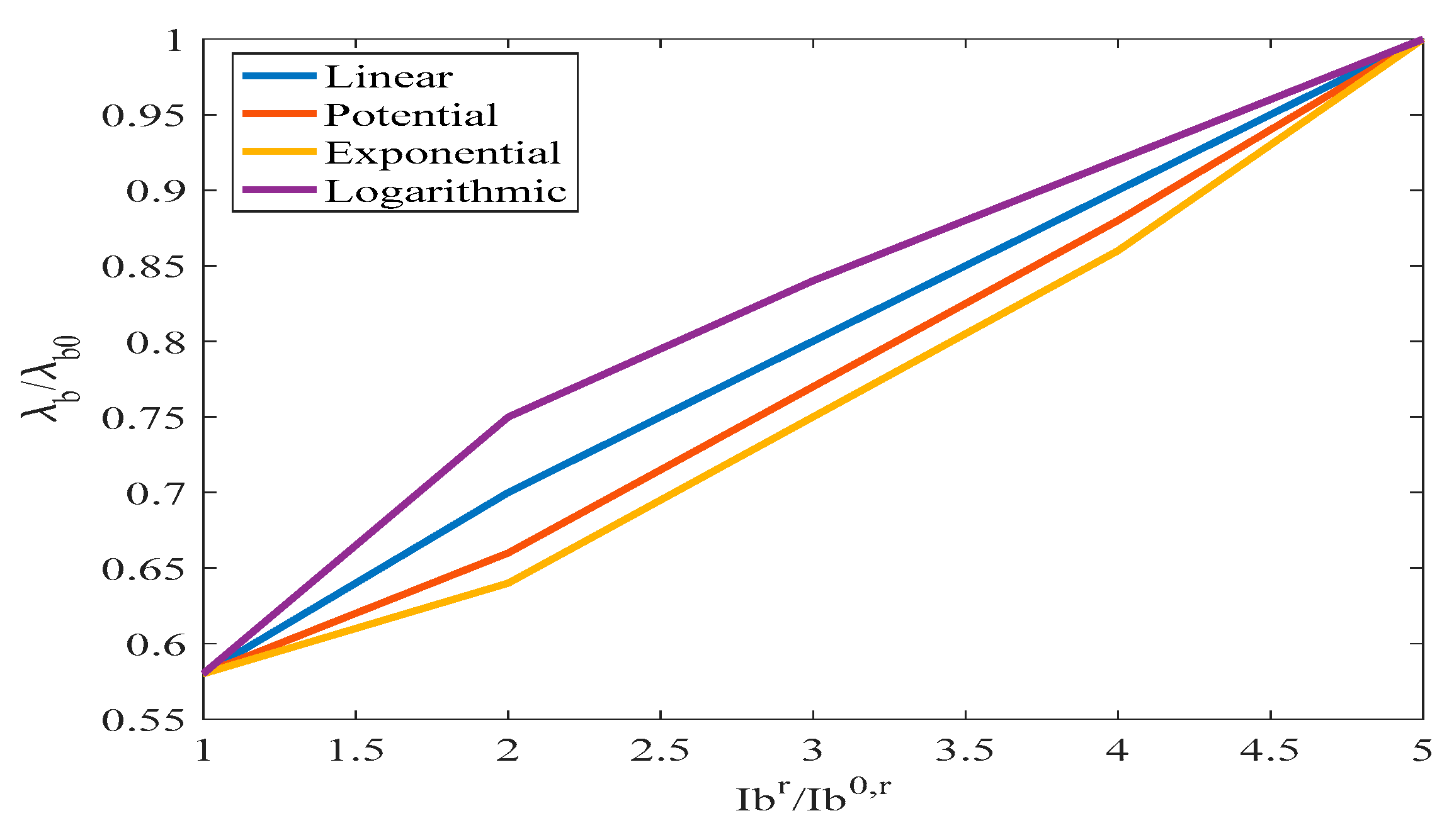
• In this work, the improvement of potential microgrid reliability due to line capacity liberalization is considered.

In the standard 34-bus distribution system, demand of 6.456 MW was adopted to evaluate the proposed method. Voltage and apparent power are the basis of choice for 12.66 kV and 100 MV analysis.

4.2. Results and Numerical Analysis

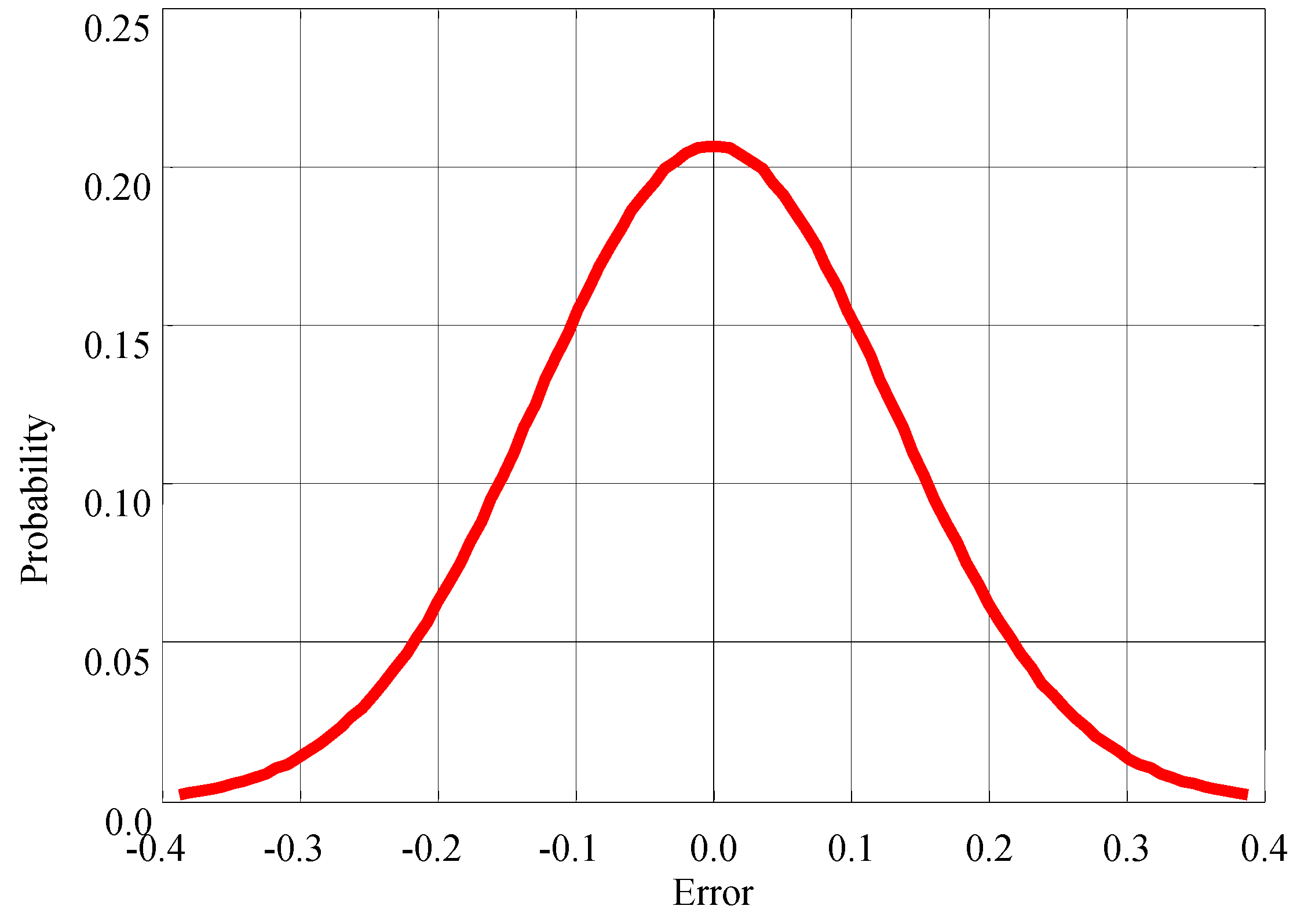
In this paper, the base’s sweep load method is modified to consider the dispersed production units. To implement the proposed method, first, the number, type, size, and location of distributed generation units and reactive power sources are obtained. It should be noted that the amount of resource capacity obtained to some extent makes the results more practical with capacities close to it. Since the problem of zoning by the graph to obtain the boundaries of the areas to install the power switch depends on the first step of the network designer, scenarios are considered, and it cannot be divided into more than four areas. The results will be presented in three scenarios.

(A) The first scenario

The maximum number of areas is divided into four areas. Figure 8 reveals the network under study and the scope of each area.

Table 3. Specifications of resources installed in the network in terms of $\mathrm{kW}$ and $\mathrm{kVAr}$.

Microgrid	$\mathbf{Place}\mathit{D}\mathit{G}$	$\mathbf{Type}\mathit{D}\mathit{G}$	$\mathbf{Size}\mathit{D}\mathit{G}$	$\mathbf{Source}\mathbf{Location}\mathit{Q}$	Source Size Q
1	3, 4	$FC,WT$	500, 300	2 $(FC)$	440
2	8, 11	$WT,FC$	432, 498	12 $(FC)$	439
3	17, 20	$FC,FC$	476, 300	23, 21 $(FC)$	495, 600
4	25, 28, 33	$WT,PV,FC$	421, 532, 602	34, 33 $(FC)$	456, 575

presents the locations of distributed generation sources and the location of sources and their size. In this table, the second column shows the location of the scattered products, the third column shows their type, and the fourth column shows their capacity. The fifth column shows the location of reactive power sources, including the capacitor or reactive power injected by the fuel cell, and the last column shows the amount of the reactive power.

Table 4. Expected unmet energy supply (in terms of $\mathrm{MWh}$ and $\mathrm{MVArh}$ ) due to lack of active and reactive power.

Microgrid	$\mathit{E}\mathit{N}{\mathit{S}}_{\mathit{P}}$	$\mathit{E}\mathit{N}{\mathit{S}}_{\mathit{Q}}$	$\mathit{E}\mathit{V}{\mathit{S}}_{\mathit{P}}$	$\mathit{E}\mathit{V}{\mathit{S}}_{\mathit{Q}}$
1	47.32	7.18	47.18	9.32
2	42.72	5.03	38.53	6.45
3	21.95	3.43	22.07	4.57
4	18.74	4.65	17.84	3.53

lists the unsupplied energy in each area. The total cost of operation, the expected cost of disconnecting the customer, and the average total loss for operation, in this case, are USD 23.15 billion, USD 2.54 million, and 91.10 kW. Reactive power effects on the depletion of line capacity to improve reliability are considered. Otherwise, the expected cut-off cost will be higher than the actual amount obtained and equal USD 3.12 million.

(B) The second scenario

In this scenario, the network is divided into three areas by changing the initial conjecture. Figure 9 depicts the network under study and the scope of each area.

Table 5. Specifications of resources installed in the network in terms of $\mathrm{kW}$ and $\mathrm{kVAr}$.

Microgrid	$\mathbf{Place}\mathit{D}\mathit{G}$	$\mathbf{Type}\mathit{D}\mathit{G}$	$\mathbf{Size}\mathit{D}\mathit{G}$	$\mathbf{Source}\mathbf{Location}\mathit{Q}$	$\mathbf{Source}\mathbf{Size}\mathit{Q}$
1	11, 7, 5, 2	$FC,PV.WT,PV$	332, 386, 342, 632	$5,(FC)$2	453, 322
2	25, 23, 22	$FC,FC,PV,PV$	268, 332, 564, 621	$21(FC)$$,19(FC)$	321, 298
3	35, 31, 27, 25	$FC,PV,WT,WT$	267, 432, 610, 457	$34,28(FC)$	465, 298

presents the locations of distributed generation sources and their types and size.

Table 6. Expected unmet energy supply (in terms of $\mathrm{MWh}$ and $\mathrm{MVArh}$ ) due to lack of active and reactive power.

Microgrid	$\mathit{E}\mathit{N}{\mathit{S}}_{\mathit{P}}$	$\mathit{E}\mathit{N}{\mathit{S}}_{\mathit{Q}}$	$\mathit{E}\mathit{V}{\mathit{S}}_{\mathit{P}}$	$\mathit{E}\mathit{V}{\mathit{S}}_{\mathit{Q}}$
1	88.32	11.29	92.32	17.25
2	42.21	8.52	43.54	5.64
3	15.54	3.32	20.86	3.68

lists the unsupplied energy in each area. The total cost of operation, the expected cost of disconnecting the customer, and the average total loss for operation, in this case, are USD 17.12 billion, USD 3.12 million, and 54,029 kW. It should be noted that the amount of cut-off cost without considering the capacity of the lines due to local compensation of reactive power is USD 3.24 million.

(C) The third scenario

In the last scenario, by selecting another number for the first region, the last possible state is obtained, including two regions. Figure 10 shows the studied network and the scope of each area.

Table 7. Specifications of resources installed in the network by $\mathrm{kVAr}$ and $\mathrm{kW}$.

Microgrid	$\mathbf{Place}\mathit{D}\mathit{G}$	$\mathbf{Type}\mathit{D}\mathit{G}$	$\mathbf{Size}\mathit{D}\mathit{G}$	$\mathbf{Source}\mathbf{Location}\mathit{Q}$	$\mathbf{Source}\mathbf{Size}\mathit{Q}$
1	2, 5, 6, 7, 15	$WT,PV,WT,FC,FC$	473, 387, 498, 428, 592, 445	8, 2 (FC),16 (FC)	387, 399, 386
2	16, 24, 26, 31, 34	$FC,WT,FC,FC,WT$	427, 489, 433, 429, 459	17 (FC), 27 (FC), 33 (FC), 34	400,395,376,310

presents the optimal locations of distributed generation sources and their type and size.

Table 8. Expected unmet energy supply (in terms of $\mathrm{MWh}$ and $\mathrm{MVArh}$ ) due to lack of active and reactive power.

Microgrids	$\mathit{E}\mathit{N}{\mathit{S}}_{\mathit{P}}$	$\mathit{E}\mathit{N}{\mathit{S}}_{\mathit{Q}}$	$\mathit{E}\mathit{V}{\mathit{S}}_{\mathit{P}}$	$\mathit{E}\mathit{V}{\mathit{S}}_{\mathit{Q}}$
1	16/52	24/23	175/57	30/36
2	55/83	8/89	56/23	8/19

lists the unsupplied energy in each area. The total cost of operation, the expected cost of disconnecting the customer, and the average total losses for operation, in this case, are USD 32.16 billion, USD 4.87 million, and 148.09 kW. The estimated cut-off cost, excluding line capacity depletion due to local reactive power compensation, is USD 5.89 million.

Different modes are possible for zoning. By comparing these three cases from the point of view of reliability index and total costs, zoning of the network into two microgrids will have high investment costs and cut-off costs, which result from the high unsupplied energy due to lack of active, reactive power according to Table 8. Therefore, this state of topology will not be appropriate. However, for the case where the network is divided into three and four microgrids, it is observed that the zoning of the system is divided into four microgrids in low supply, as detailed in Table 4. In addition, the design of three microgrids will have fewer losses, indicating that this design is more appropriate. For a better comparison, in

Table 9. Comparison of design with the creation of different microgrids.

Number of Microgrids	Total Cost	${\mathit{E}}_{\mathbf{cos}\mathit{t}}$	Losses	$\mathbf{Reactive}{\mathit{E}}_{\mathbf{cos}\mathit{t}}\mathbf{without}\mathbf{Power}\mathbf{Compensation}$
2	23.15	2.54	91.10	3.12
3	17.12	3.12	54.029	3.24
4	32.16	4.87	148.09	5.89

, the design results are given to create the number of different microgrids.

4.3. Error Analysis

To investigate the reliability of the study distribution system, errors are considered in different parts of the system. For this purpose, assuming that the fault location is detected in the ground state where the network is not zoned, the downstream fault network is separated so that the fault-free parts can be exploited. However, in the zoned state, even with the separation of the lower part, more than 70% of the microgrid load is provided. It should be noted that because the steady-state conditions of the system are considered in the design, the dynamics and transient state of the system are not considered. Therefore, the operator can prevent the shutdown of the microgrids created by using two corrective actions to remove the load and increase the non-probabilistic production. For this purpose, three errors were applied in each of the three microgrids obtained from Scenario 2. Assuming that the first error is in the first microgrid and the range of 2 to 11 buses, if the network is not operating as a microgrid, all the buses after the error will be located without electricity. However, in the microgrid mode, the second and third microgrids will be located. They can be retrieved after an error occurs and disconnected from the upstream area and provide other network loads as an island by eliminating lower priority loads. Suppose the error occurs in the second microgrid, e.g., in the range of 13 to 23, after recovery. In that case, only the microgrid between the error and the start of the third microgrid will be without electricity. The necessary loads of the third microgrid will be provided with a suitable reloading plan. In the end, with an error in the third microgrid in the range of 25 to 34 buses from the fault location to the end of the network, all these loads will be disconnected, and in this case, there is no difference in the middle of any of the operating modes. In

Table 10. Error analysis in the designed microgrid.

Type of Operation	Error (%)	$\mathit{E}\mathit{N}{\mathit{S}}_{\mathit{P}}$	$\mathit{E}\mathit{N}{\mathit{S}}_{\mathit{Q}}$	$\mathit{V}\mathit{N}{\mathit{S}}_{\mathit{Q}}$	$\mathit{V}\mathit{N}{\mathit{S}}_{\mathit{Q}}$
Traditional distribution system	5	142.21	19.32	144.32	25.28
	18	75.24	10.24	81.54	12.65
	30	27.06	4.57	25.75	4.32
Microgrid	5	101.45	13.67	112.15	15.51
	18	64.79	6.13	71.28	10.78
	30	26.37	3.25	26.32	4.32

, for example, an error is applied in each microgrids, and the reliability index is evaluated in the two cases mentioned.

At the same time, the investment cost of installing circuit breakers and creating separate operating centers for each microgrid to create the ability to become an island is cost-effective in terms of improving network reliability due to the return on the investment use of renewable products. Therefore, the importance of considering the issue of planning combined with the zoning of current conventional networks and the transition to new self-sufficient microgrids is evident.

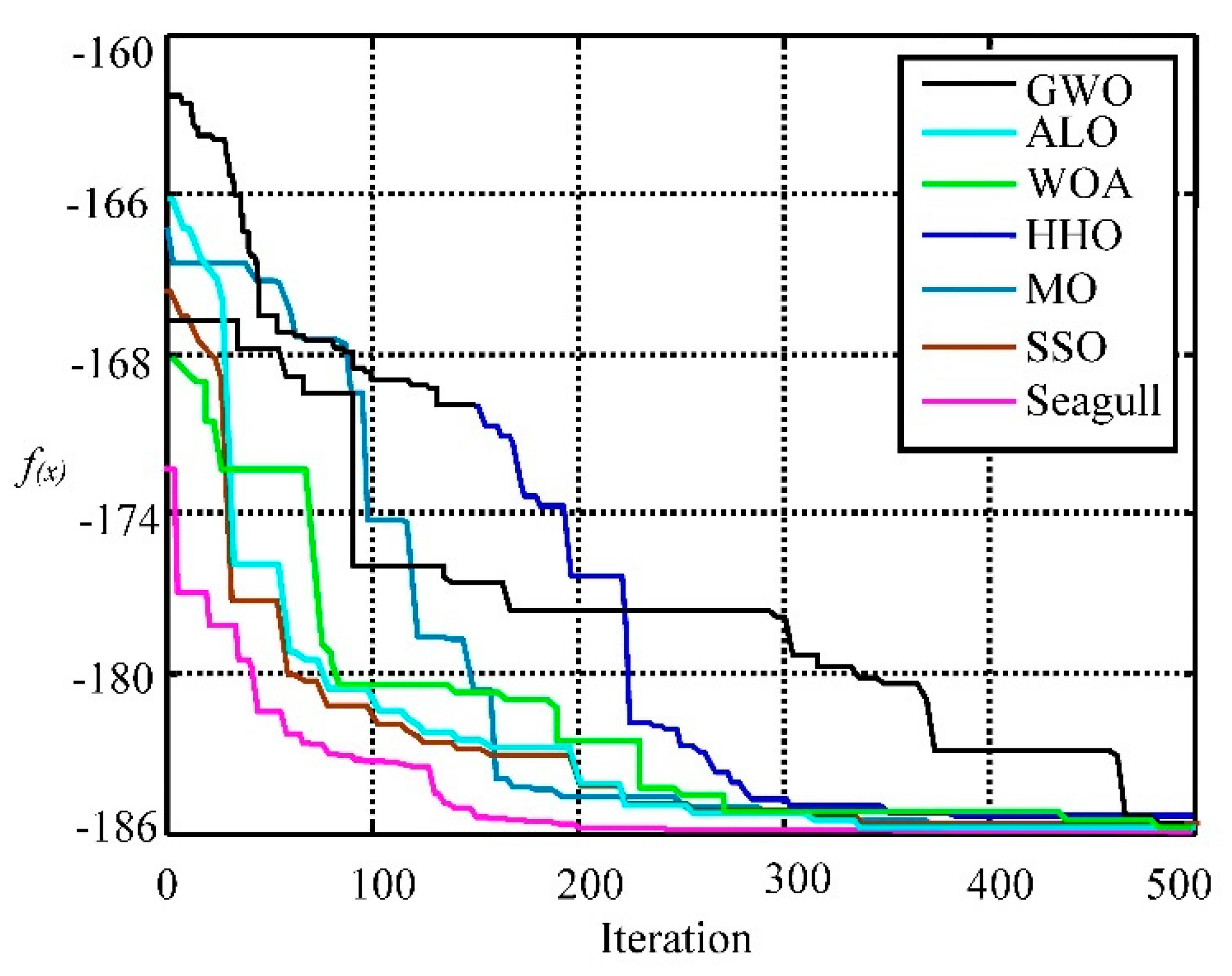
4.4. Algorithm Analysis

The optimal coefficients of the suggested model are obtained by various test functions. The first initial population is 60, σ = 0.3, λ = N/2, repetition is 300, and the results are compared with NSGA, SPEA, and MOPSO models. The convergence of the optimal Pareto set (C-metric (C): C-metric) to cover the above objectives is considered:

Suppose S₁ and $S_2\subseteq S$ sets of answers and C-metric is pairs $(S_1,S_2)$ and $[0,1]$ distances according to the following relation:

$$C(S_1,S_2)=\frac{\left|\right\{a_2\in S_2,\exists a_1\in S_1:a_1\prec a_2\left\}\right|}{\left|S_2\right|}$$

(61)

If $C(S_1,S_2)=1$, answers in set S₂ override the answers S₁. If $C(S_1,S_2)=0$, no S₂ answers are covered via S₁. Both $C(S_1,S_2)$ and $C(S_2,S_1)$ are compared, and obtained data are presented in

Table 11. Comparison of algorithms based on C-metric criteria.

	C(B1,B2)	C(B2,B1)	C(B1,B3)	C(B3,B1)	C(B1,B4)	C(B4,B1)
Best	0.752	0.0038	0.524	0.0214	0.501	0.0318
Average	0.683	0.001112	0.502	0.0238	0.483	0.0315
Std	0.0029	0.00012	0.0036	0.00021	0.00221	0.00012

. The NSGA, SPEA, and MOPSO are the mean values of 68.3%, 50.2%, and 48.3%, which are covered by our model. According to the data presented in Table 5, our model is worked better than other models.

The following test function was selected to compare the performance of the proposed method, GWO, ALO, WOA, Harris Hawks Optimizer (HHO), Moth optimization (MO), and sine cosine optimization (SSO):

$$f(x)=({\displaystyle \sum _{i=1}^{5}i\cos ((i+1)x_1+i)})({\displaystyle \sum _{i=1}^{5}i\cos ((i+1)x_2+i)})$$

(62)

The reason for choosing this function is the existence of local points and flat plates and its many valleys and peaks. Figure 11 demonstrates a 3D view to better understand this function. It should be noted that the minimum value of this function is equal to −7309/186. To make a good comparison between the proposed methods, the number of initial populations and repetition of the program for all sexes are equal to 50 and 200, respectively. Figure 12 shows a convergence comparison of the methods used. From the obtained results, it can be seen that the proposed method achieves convergence in less time and, at the same time, gives a better optimal answer compared to other methods. From the closeness between the maximum and the minimum answer, it can be seen that the proposed algorithm has less standard deviation, which indicates its better resistance to solving the optimization problem.

5. Conclusions

In the planning step for distribution networks, the optimal design of microgrids is a crucial matter. One of the most critical goals in the design of microgrids is to provide a load with the highest reliability and lowest cost. The construction of microgrids in the distribution system has many advantages in minimizing the interaction between the microgrids, preventing the progression of errors, and ultimately increasing the reliability of consumers and distribution companies. In this research study, considering the importance of both cost and reliability aspects, several approaches are created and compared to optimally design the concept of microgrids in an active distribution network. Initially, the distribution system is developed by introducing different types of units, such as wind turbines, solar generators, and fuel cell generators. Due to the nature of renewable sources and hourly load characteristics, these products’ appropriate location and size to minimize total losses and cost and reliability criteria are optimally determined. Simultaneously, by using graph theory and obtaining the zoning matrix, the system is divided into optimal microgrids that are modified to consider different areas of the indicators. Since such a problem has its own complexity, the developed Seagull algorithm is used to solve it. In this algorithm, the concept of dynamic archiving with the ability to store non-dominant Pareto answers is used. The roulette cycle method is used to find suitable archived answers. Finally, the proposed method and model for a sample system in different scenarios are discussed. Various zoning scenarios were considered to obtain the best zoning mode and the most reliable microgrid considering the costs. This strategy will make it easier to control each microgrid and protect healthy areas of the network during disruptions. In addition, in most studies, the problem is seen as a single objective using weighting coefficients. However, as can be seen here, the importance of considering the conflict between goals is unavoidable. Therefore, since the third approach provides more choices for the system designer, and it usually makes more sense to consider several goals simultaneously in practice, the third approach is better than the first and second approaches.

According to the hypothetical errors, the comparison of the corresponding rows in the table above shows that in the programming mode—considering the island capability, for example, $EN{S}_P$, $EN{S}_Q$, $VN{S}_Q$, and $VN{S}_P$, the index for the first error was improved by 29.67, 31.37, 25.32, and 35.12%, respectively. For other errors, improvements are also observed.

In future work, the presence of electric vehicles and energy storage resources as equipment used in microgrids to implement demand-side management programs will be discussed. In addition, the environmental pollution along with the economic aspect and reliability can be discussed.

References

1. Paliwal, P. Securing Reliability Constrained Technology Combination for Isolated Micro-Grid Using Multi-Agent Based Optimization. Iran. J. Electr. Electron. Eng. 2022, 18, 2180. [Google Scholar]
2. Mishra, S.; Bordin, C.; Tomasgard, A.; Palu, I. A multi-agent system approach for optimal microgrid expansion planning under uncertainty. Int. J. Electr. Power Energy Syst. 2019, 109, 696–709. [Google Scholar] [CrossRef]
3. Kiran, R.S.; Reddy, S.S. A mixed integer optimization model for reliability indices enhancement in Micro-grid system with renewable generation and energy storage. Mater. Today Proc. 2021, in press. [Google Scholar] [CrossRef]
4. Nayeripour, M.; Hasanvand, S.; Fallahzadeh-Abarghouei, H. Capacity Expansion Planning with Respect to Reliability in Order to Transform an Existing Distribution Network into Micro-Grid. Tabriz J. Electr. Eng. 2017, 47, 761–774. [Google Scholar]
5. Cheng, L.; Wan, Y.; Qi, N.; Zhou, Y. Coordinated operation strategy of distribution network with the multi-station integrated system considering the risk of controllable resources. Int. J. Electr. Power Energy Syst. 2022, 137, 107793. [Google Scholar] [CrossRef]
6. Navidi, M.; Moghaddas Tafreshi, S.M.; Anvari-Moghaddam, A. Sub-Transmission Network Expansion Planning Considering Regional Energy Systems: A Bi-Level Approach. Electronics 2019, 8, 1416. [Google Scholar] [CrossRef] [Green Version]
7. Khan, B.; Alhelou, H.H.; Mebrahtu, F. A holistic analysis of distribution system reliability assessment methods with conventional and renewable energy sources. AIMS Energy 2019, 7, 413–429. [Google Scholar] [CrossRef]
8. Su, S.; Hu, Y.; He, L.; Yamashita, K.; Wang, S. An assessment procedure of distribution network reliability considering photovoltaic power integration. IEEE Access 2019, 7, 60171–60185. [Google Scholar] [CrossRef]
9. Gomes, P.V.; Saraiva, J.T. State-of-the-art of transmission expansion planning: A survey from restructuring to renewable and distributed electricity markets. Int. J. Electr. Power Energy Syst. 2019, 111, 411–424. [Google Scholar] [CrossRef]
10. Javadi, M.S.; Esmaeel Nezhad, A. Multi-objective, multi-year dynamic generation and transmission expansion planning-renewable energy sources integration for Iran’s National Power Grid. Int. Trans. Electr. Energy Syst. 2019, 29, e2810. [Google Scholar] [CrossRef]
11. Pourjamal, Y.; Ajami, A. A novel approach to minimizing power losses and improving reliability through DG placement and sizing. J. Electr. Eng. 2001, 42, 1–11. [Google Scholar]
12. Lakum, A.; Mahajan, V. A novel approach for optimal placement and sizing of active power filters in radial distribution system with nonlinear distributed generation using adaptive grey wolf optimizer. Eng. Sci. Technol. Int. J. 2021, 24, 911–924. [Google Scholar] [CrossRef]
13. Iris, Ç.; Lam, J.S.L. Optimal energy management and operations planning in seaports with smart grid while harnessing renewable energy under uncertainty. Omega 2021, 103, 102445. [Google Scholar] [CrossRef]
14. Khazaei, J. Optimal Flow of MVDC Shipboard Microgrids with Hybrid Storage Enhanced with Capacitive and Resistive Droop Controllers. IEEE Trans. Power Syst. 2021, 36, 3728–3739. [Google Scholar] [CrossRef]
15. Panda, A.; Mishra, U.; Aviso, K.B. Optimizing hybrid power systems with compressed air energy storage. Energy 2020, 205, 117962. [Google Scholar] [CrossRef]
16. Tooryan, F.; HassanzadehFard, H.; Collins, E.R.; Jin, S.; Ramezani, B. Smart integration of renewable energy resources, electrical, and thermal energy storage in microgrid applications. Energy 2020, 212, 118716. [Google Scholar] [CrossRef]
17. Hong, Y.Y.; Apolinario, G.F.D. Uncertainty in Unit Commitment in Power Systems: A Review of Models, Methods, and Applications. Energies 2021, 14, 6658. [Google Scholar] [CrossRef]
18. Sepehrzad, R.; Mahmoodi, A.; Ghalebi, S.Y.; Moridi, A.R.; Seifi, A.R. Intelligent hierarchical energy and power management to control the voltage and frequency of micro-grids based on power uncertainties and communication latency. Electr. Power Syst. Res. 2022, 202, 107567. [Google Scholar] [CrossRef]
19. Nandi, A.; Kamboj, V.K.; Khatri, M. Hybrid chaotic approaches to solve profit based unit commitment with plug-in electric vehicle and renewable energy sources in winter and summer. Mater. Today Proc. 2022, in press. [Google Scholar] [CrossRef]
20. Riou, M.; Dupriez-Robin, F.; Grondin, D.; Le Loup, C.; Benne, M.; Tran, Q.T. Multi-Objective Optimization of Autonomous Microgrids with Reliability Consideration. Energies 2021, 14, 4466. [Google Scholar] [CrossRef]
21. Guo, L.; Liu, W.; Jiao, B.; Hong, B.; Wang, C. Multi-objective stochastic optimal planning method for stand-alone microgrid system. IET Gener. Transm. Distrib. 2014, 8, 1263–1273. [Google Scholar] [CrossRef]
22. Wang, Z.; Chen, B.; Wang, J.; Chen, C. Networked microgrids for self-healing power systems. IEEE Trans. Smart Grid 2015, 7, 310–319. [Google Scholar] [CrossRef]
23. Wang, Z.; Wang, J. Self-healing resilient distribution systems based on sectionalization into microgrids. IEEE Trans. Power Syst. 2015, 30, 3139–3149. [Google Scholar] [CrossRef]
24. Prabatha, T.; Karunathilake, H.; Shotorbani, A.M.; Sadiq, R.; Hewage, K. Community-level decentralized energy system planning under uncertainty: A comparison of mathematical models for strategy development. Appl. Energy 2021, 283, 116304. [Google Scholar] [CrossRef]
25. Dai, Y.; Ma, X.; Hu, Z.; Li, Z.; Li, Y. Optimization of Deep Belief Network and Its Application on Equivalent Modeling for Micro-Grid. In Proceedings of the 2021 40th Chinese Control Conference (CCC), Shanghai, China, 26–28 July 2021; pp. 1224–1229. [Google Scholar]
26. Nispel, A.; Ekwaro-Osire, S.; Dias, J.P.; Cunha, A. Uncertainty Quantification for Fatigue Life of Offshore Wind Turbine Structure. ASCE-ASME J. Risk Uncertain. Eng. Syst. Part B Mech. Eng. 2021, 7, 040901. [Google Scholar] [CrossRef]
27. Rezaei, N.; Pezhmani, Y.; Khazali, A. Economic-environmental risk-averse optimal heat and power energy management of a grid-connected multi microgrid system considering demand response and bidding strategy. Energy 2022, 240, 122844. [Google Scholar] [CrossRef]
28. Upadhyaya, P.; Jarlbering, E.; Tudisco, F. The self-consistent field iteration for p-spectral clustering. arXiv 2021, arXiv:2111.09750. [Google Scholar]
29. Rahmani-andebili, M. Reliability and economic-driven switchable capacitor placement in distribution network. IET Gener. Transm. Distrib. 2015, 9, 1572–1579. [Google Scholar] [CrossRef]
30. Qin, W.; Wang, P.; Han, X.; Du, X. Reactive power aspects in reliability assessment of power systems. IEEE Trans. Power Syst. 2010, 26, 85–92. [Google Scholar] [CrossRef]
31. Nayeripour, M.; Fallahzadeh-Abarghouei, H.; Hasanvand, S.; Hassanzadeh, M.E. Interactive fuzzy binary shuffled frog leaping algorithm for multi-objective reliable economic power distribution system expansion planning. J. Intell. Fuzzy Syst. 2015, 29, 351–363. [Google Scholar] [CrossRef]
32. Ramesh, S.; Kannan, S.; Baskar, S. Application of modified NSGA-II algorithm to multi-objective reactive power planning. Appl. Soft Comput. 2012, 12, 741–753. [Google Scholar] [CrossRef]
33. Wang, S.; Li, Z.; Wu, L.; Shahidehpour, M.; Li, Z. New metrics for assessing the reliability and economics of microgrids in distribution system. IEEE Trans. Power Syst. 2013, 28, 2852–2861. [Google Scholar] [CrossRef]
34. Atwa, Y.M.; El-Saadany, E.F.; Salama, M.M.A.; Seethapathy, R.; Assam, M.; Conti, S. Adequacy evaluation of distribution system including wind/solar DG during different modes of operation. IEEE Trans. Power Syst. 2011, 26, 1945–1952. [Google Scholar] [CrossRef]
35. Surya, V.; Senthilselvi, A. Identification of oil authenticity and adulteration using deep long short-term memory-based neural network with seagull optimization algorithm. Neural Comput. Appl. 2022, 34, 7611–7625. [Google Scholar] [CrossRef]
36. Li, B.; Tian, X.; Zhang, M. Modeling and multi-objective optimization method of machine tool energy consumption considering tool wear. Int. J. Precis. Eng. Manuf. Green Technol. 2022, 9, 127–141. [Google Scholar] [CrossRef]
37. Willis, H.L. Power Distribution Planning Reference Book; CRC Press: Boca Raton, FL, USA, 1997. [Google Scholar]
Figure 1. Hourly load factor curve.
Applsci 12 04743 g001
Figure 2. Monthly load factor curve.
Applsci 12 04743 g002
Figure 3. The amount of peak load per bus.
Applsci 12 04743 g003
Figure 4. Production power and wind speed.
Applsci 12 04743 g004
Figure 5. Density function of production probability by PV.
Applsci 12 04743 g005
Figure 6. Branch failure rate (pu) versus reactive current component (pu).
Applsci 12 04743 g006
Figure 7. Flowchart of the proposed method in problem-solving.
Applsci 12 04743 g007
Figure 8. Network zoning to 4 microgrids. Which each zone in separated with different colors.
Applsci 12 04743 g008
Figure 9. Network zoning into 3 microgrids. Which each zone in separated with different colors.
Applsci 12 04743 g009
Figure 10. Network zoning into 2 microgrids in the third scenario. Which each zone in separated with different colors.
Applsci 12 04743 g010
Figure 11. Three-dimensional view of the standard test function.
Applsci 12 04743 g011
Figure 12. Convergence of proposed methods to solve the standard test function.
Applsci 12 04743 g012