
Countrywide Mapping of Plant Ecological Communities with 101 Legends including Land Cover Types for the First Time at 10 m Resolution through Convolutional Learning of Satellite Images


Abstract
:1. Introduction
2. Materials and Methods
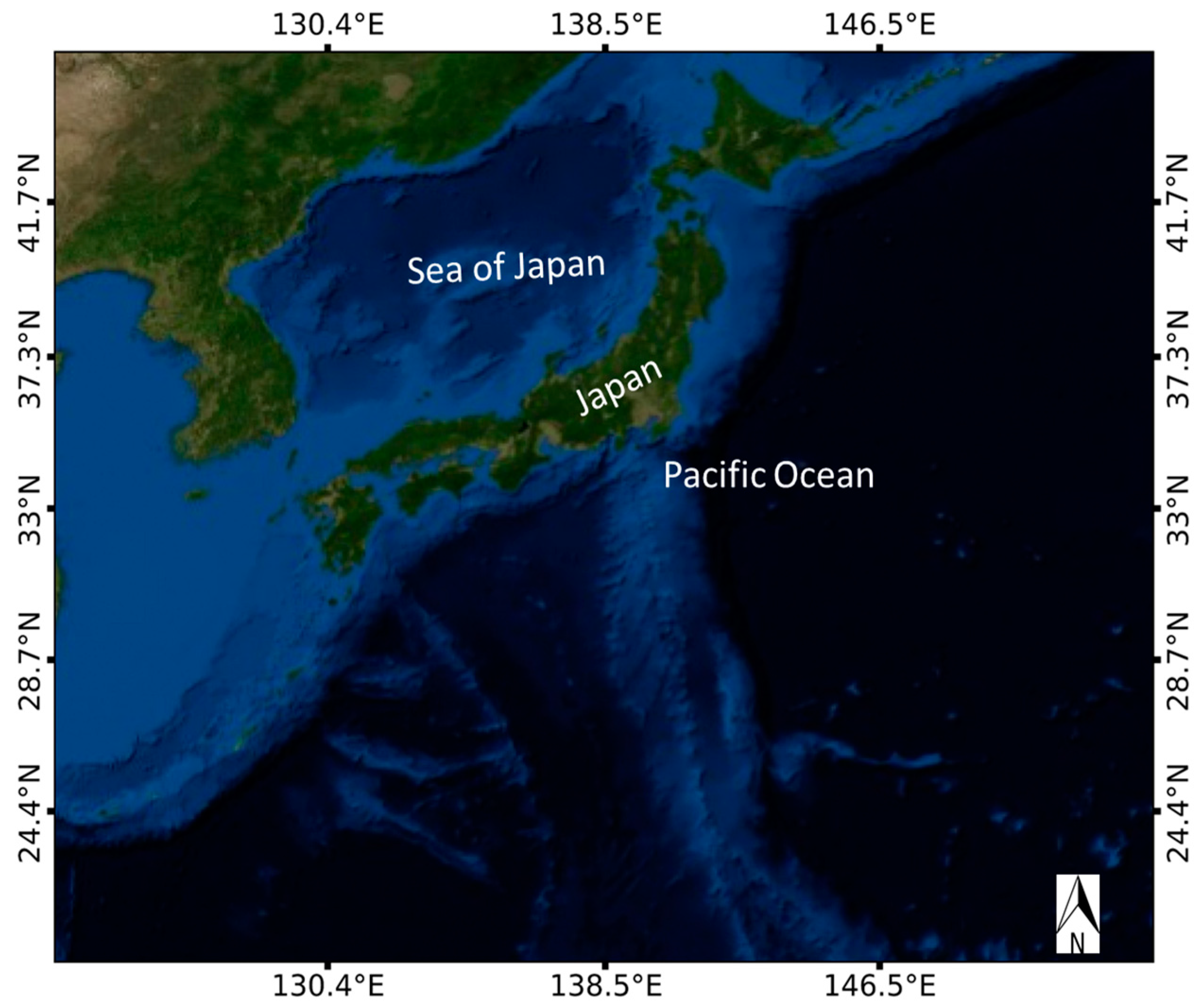
2.1. Study Area
2.2. Preparation of Ground Truth Data
2.3. Processing of Satellite Data
2.4. Deep Convolutional Learning and Mapping
3. Results
3.1. Cross-Validation Accuracies
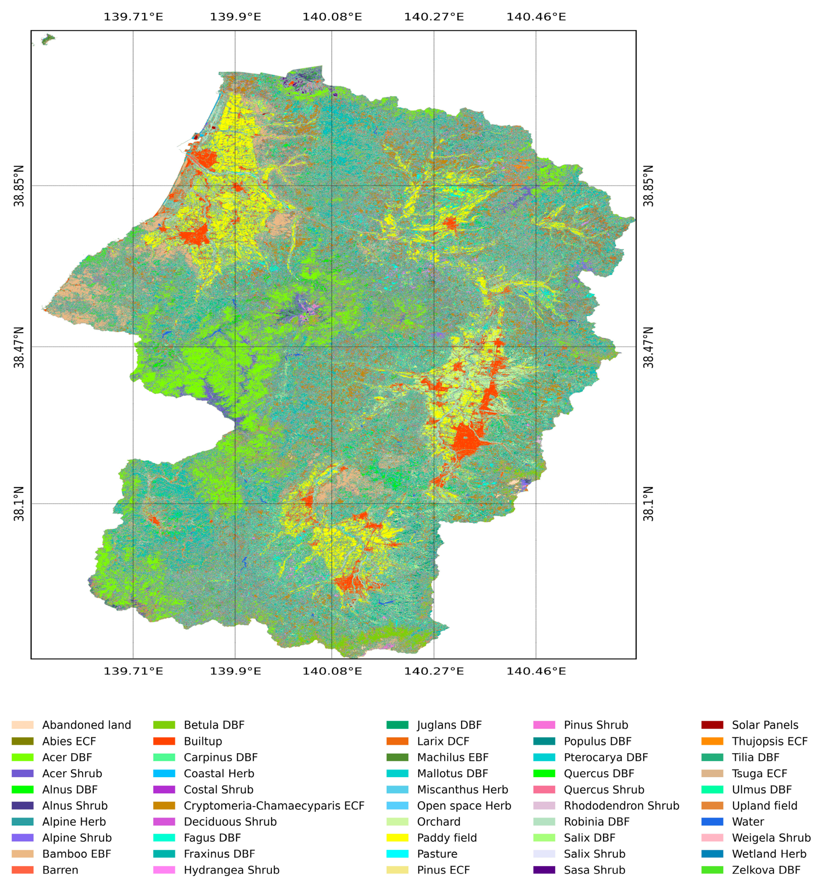
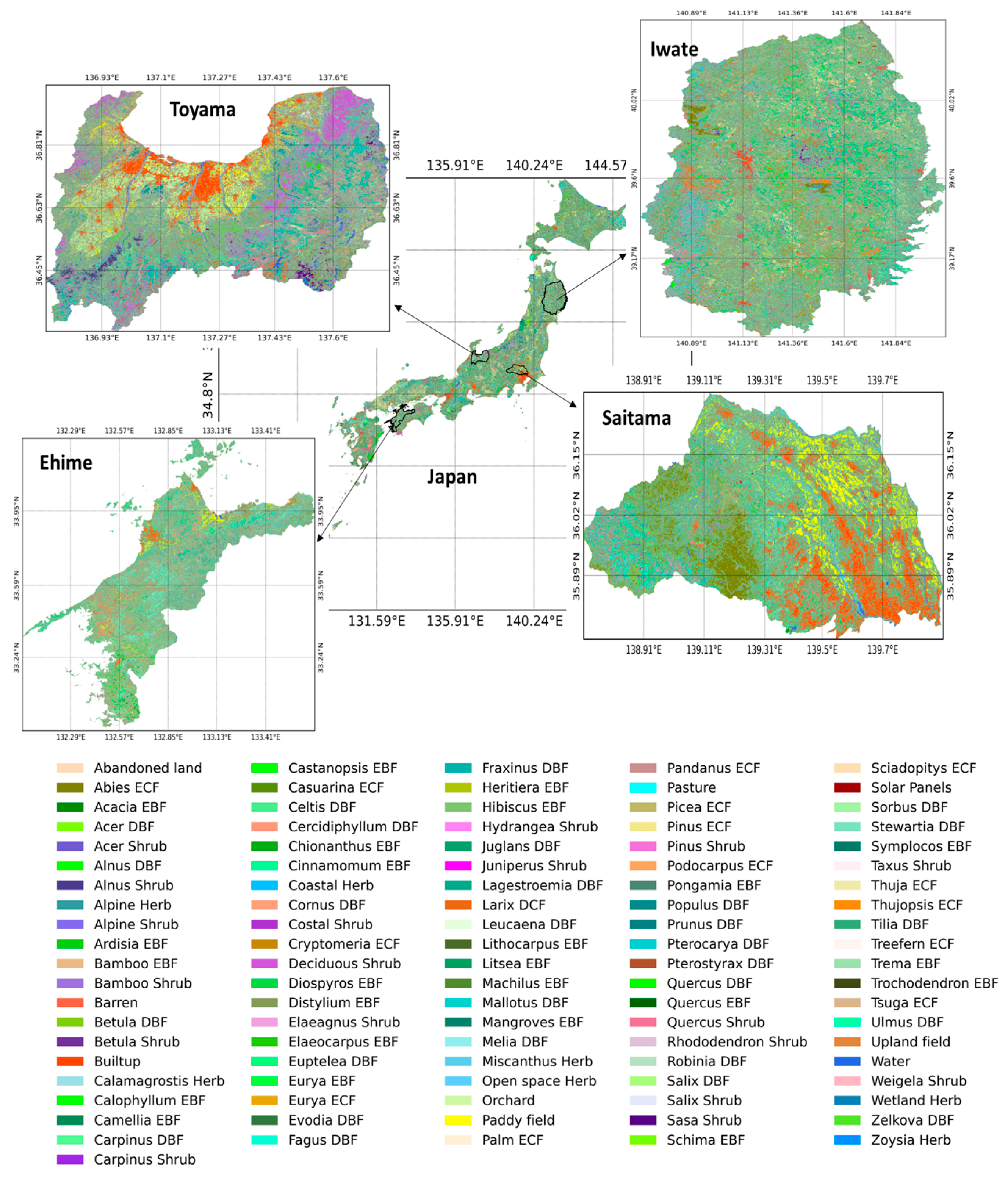
3.2. Prefecture-Wise Ecological Communities Maps
3.3. Countrywide Distribution of Ecological Communities
4. Discussion
5. Conclusions
Supplementary Materials
Funding
Acknowledgments
Conflicts of Interest
References
- Foley, J.A.; DeFries, R.; Asner, G.P.; Barford, C.; Bonan, G.; Carpenter, S.R.; Chapin, F.S.; Coe, M.T.; Daily, G.C.; Gibbs, H.K.; et al. Global Consequences of Land Use. Science 2005, 309, 570–574. [Google Scholar] [CrossRef] [Green Version]
- Chen, B.; Zhang, X.; Tao, J.; Wu, J.; Wang, J.; Shi, P.; Zhang, Y.; Yu, C. The Impact of Climate Change and Anthropogenic Activities on Alpine Grassland over the Qinghai-Tibet Plateau. Agric. For. Meteorol. 2014, 189–190, 11–18. [Google Scholar] [CrossRef]
- Lehosmaa, K.; Jyväsjärvi, J.; Virtanen, R.; Ilmonen, J.; Saastamoinen, J.; Muotka, T. Anthropogenic Habitat Disturbance Induces a Major Biodiversity Change in Habitat Specialist Bryophytes of Boreal Springs. Biol. Conserv. 2017, 215, 169–178. [Google Scholar] [CrossRef]
- Grimm, N.B.; Chapin, F.S.; Bierwagen, B.; Gonzalez, P.; Groffman, P.M.; Luo, Y.; Melton, F.; Nadelhoffer, K.; Pairis, A.; Raymond, P.A.; et al. The Impacts of Climate Change on Ecosystem Structure and Function. Front. Ecol. Environ. 2013, 11, 474–482. [Google Scholar] [CrossRef] [Green Version]
- Schirpke, U.; Kohler, M.; Leitinger, G.; Fontana, V.; Tasser, E.; Tappeiner, U. Future Impacts of Changing Land-Use and Climate on Ecosystem Services of Mountain Grassland and Their Resilience. Ecosyst. Serv. 2017, 26, 79–94. [Google Scholar] [CrossRef] [PubMed]
- Li, D.; Wu, S.; Liu, L.; Zhang, Y.; Li, S. Vulnerability of the Global Terrestrial Ecosystems to Climate Change. Glob. Chang. Biol. 2018, 24, 4095–4106. [Google Scholar] [CrossRef]
- Kuchler, A.W. Problems in Classifying and Mapping Vegetation for Ecological Regionalization. Ecology 1973, 54, 512–523. [Google Scholar] [CrossRef]
- Henderson, E.B.; Bell, D.M.; Gregory, M.J. Vegetation Mapping to Support Greater Sage-grouse Habitat Monitoring and Management: Multi- or Univariate Approach? Ecosphere 2019, 10, e02838. [Google Scholar] [CrossRef]
- Schrodt, F.; de la Barreda Bautista, B.; Williams, C.; Boyd, D.S.; Schaepman-Strub, G.; Santos, M.J. Integrating Biodiversity, Remote Sensing, and Auxiliary Information for the Study of Ecosystem Functioning and Conservation at Large Spatial Scales. In Remote Sensing of Plant Biodiversity; Cavender-Bares, J., Gamon, J.A., Townsend, P.A., Eds.; Springer International Publishing: Cham, Switzerland, 2020; pp. 449–484. ISBN 978-3-030-33156-6. [Google Scholar]
- Bowler, D.E.; Bjorkman, A.D.; Dornelas, M.; Myers-Smith, I.H.; Navarro, L.M.; Niamir, A.; Supp, S.R.; Waldock, C.; Winter, M.; Vellend, M.; et al. Mapping Human Pressures on Biodiversity across the Planet Uncovers Anthropogenic Threat Complexes. People Nat. 2020, 2, 380–394. [Google Scholar] [CrossRef] [Green Version]
- Iverson, L.R.; Graham, R.L.; Cook, E.A. Applications of Satellite Remote Sensing to Forested Ecosystems. Landscape Ecol. 1989, 3, 131–143. [Google Scholar] [CrossRef]
- Pettorelli, N.; Schulte to Bühne, H.; Tulloch, A.; Dubois, G.; Macinnis-Ng, C.; Queirós, A.M.; Keith, D.A.; Wegmann, M.; Schrodt, F.; Stellmes, M.; et al. Satellite Remote Sensing of Ecosystem Functions: Opportunities, Challenges and Way Forward. Remote Sens. Ecol. Conserv. 2018, 4, 71–93. [Google Scholar] [CrossRef]
- Guo, X.; Coops, N.C.; Gergel, S.E.; Bater, C.W.; Nielsen, S.E.; Stadt, J.J.; Drever, M. Integrating Airborne Lidar and Satellite Imagery to Model Habitat Connectivity Dynamics for Spatial Conservation Prioritization. Landsc. Ecol. 2018, 33, 491–511. [Google Scholar] [CrossRef]
- Babí Almenar, J.; Bolowich, A.; Elliot, T.; Geneletti, D.; Sonnemann, G.; Rugani, B. Assessing Habitat Loss, Fragmentation and Ecological Connectivity in Luxembourg to Support Spatial Planning. Landsc. Urban Plan. 2019, 189, 335–351. [Google Scholar] [CrossRef]
- Fu, W.; Ma, J.; Chen, P.; Chen, F. Remote Sensing Satellites for Digital Earth. In Manual of Digital Earth; Guo, H., Goodchild, M.F., Annoni, A., Eds.; Springer: Singapore, 2020; pp. 55–123. ISBN 978-981-329-914-6. [Google Scholar]
- Rhodes, C.J.; Henrys, P.; Siriwardena, G.M.; Whittingham, M.J.; Norton, L.R. The Relative Value of Field Survey and Remote Sensing for Biodiversity Assessment. Methods Ecol. Evol. 2015, 6, 772–781. [Google Scholar] [CrossRef]
- Macintyre, P.; van Niekerk, A.; Mucina, L. Efficacy of Multi-Season Sentinel-2 Imagery for Compositional Vegetation Classification. Int. J. Appl. Earth Obs. Geoinf. 2020, 85, 101980. [Google Scholar] [CrossRef]
- Brook, R.K.; Kenkel, N.C. A Multivariate Approach to Vegetation Mapping of Manitoba’s Hudson Bay Lowlands. International J. Remote Sens. 2002, 23, 4761–4776. [Google Scholar] [CrossRef]
- Xie, Y.; Sha, Z.; Yu, M. Remote Sensing Imagery in Vegetation Mapping: A Review. J. Plant Ecol. 2008, 1, 9–23. [Google Scholar] [CrossRef]
- Ustin, S.L.; Middleton, E.M. Current and Near-Term Advances in Earth Observation for Ecological Applications. Ecol. Process 2021, 10, 1. [Google Scholar] [CrossRef]
- Adam, E.; Mutanga, O.; Rugege, D. Multispectral and Hyperspectral Remote Sensing for Identification and Mapping of Wetland Vegetation: A Review. Wetl. Ecol. Manag. 2010, 18, 281–296. [Google Scholar] [CrossRef]
- Natividade, J.; Prado, J.; Marques, L. Low-Cost Multi-Spectral Vegetation Classification Using an Unmanned Aerial Vehicle. In Proceedings of the 2017 IEEE International Conference on Autonomous Robot Systems and Competitions (ICARSC), Coimbra, Portugal, 26–28 April 2017; IEEE: Piscataway, NJ, USA, 2017; pp. 336–342. [Google Scholar]
- Langford, Z.L.; Kumar, J.; Hoffman, F.M.; Breen, A.L.; Iversen, C.M. Arctic Vegetation Mapping Using Unsupervised Training Datasets and Convolutional Neural Networks. Remote Sens. 2019, 11, 69. [Google Scholar] [CrossRef] [Green Version]
- Westinga, E.; Beltran, A.P.R.; de Bie, C.A.J.M.; van Gils, H.A.M.J. A Novel Approach to Optimize Hierarchical Vegetation Mapping from Hyper-Temporal NDVI Imagery, Demonstrated at National Level for Namibia. Int. J. Appl. Earth Obs. Geoinf. 2020, 91, 102152. [Google Scholar] [CrossRef]
- Yeo, S.; Lafon, V.; Alard, D.; Curti, C.; Dehouck, A.; Benot, M.-L. Classification and Mapping of Saltmarsh Vegetation Combining Multispectral Images with Field Data. Estuar. Coast. Shelf Sci. 2020, 236, 106643. [Google Scholar] [CrossRef]
- Lassiter, A.; Darbari, M. Assessing Alternative Methods for Unsupervised Segmentation of Urban Vegetation in Very High-Resolution Multispectral Aerial Imagery. PLoS ONE 2020, 15, e0230856. [Google Scholar] [CrossRef] [PubMed]
- Shih, H.; Stow, D.A.; Tsai, Y.H. Guidance on and Comparison of Machine Learning Classifiers for Landsat-Based Land Cover and Land Use Mapping. Int. J. Remote Sens. 2019, 40, 1248–1274. [Google Scholar] [CrossRef]
- Talukdar, S.; Singha, P.; Mahato, S.; Shahfahad; Pal, S.; Liou, Y.-A.; Rahman, A. Land-Use Land-Cover Classification by Machine Learning Classifiers for Satellite Observations—A Review. Remote Sens. 2020, 12, 1135. [Google Scholar] [CrossRef] [Green Version]
- Furuya, D.E.G.; Aguiar, J.A.F.; Estrabis, N.V.; Pinheiro, M.M.F.; Furuya, M.T.G.; Pereira, D.R.; Gonçalves, W.N.; Liesenberg, V.; Li, J.; Marcato Junior, J.; et al. A Machine Learning Approach for Mapping Forest Vegetation in Riparian Zones in an Atlantic Biome Environment Using Sentinel-2 Imagery. Remote Sens. 2020, 12, 4086. [Google Scholar] [CrossRef]
- Hamylton, S.M.; Morris, R.H.; Carvalho, R.C.; Roder, N.; Barlow, P.; Mills, K.; Wang, L. Evaluating Techniques for Mapping Island Vegetation from Unmanned Aerial Vehicle (UAV) Images: Pixel Classification, Visual Interpretation and Machine Learning Approaches. Int. J. Appl. Earth Obs. Geoinf. 2020, 89, 102085. [Google Scholar] [CrossRef]
- Pan, X.; Wang, Z.; Gao, Y.; Dang, X.; Han, Y. Detailed and Automated Classification of Land Use/Land Cover Using Machine Learning Algorithms in Google Earth Engine. Geocarto Int. 2021. [Google Scholar] [CrossRef]
- Breiman, L. Random Forests. Mach. Learn. 2001, 45, 5–32. [Google Scholar] [CrossRef] [Green Version]
- Chang, C.-C.; Lin, C.-J. LIBSVM: A Library for Support Vector Machines. ACM Trans. Intell. Syst. Technol. 2011, 2, 1–27. [Google Scholar] [CrossRef]
- Chen, T.; Guestrin, C. XGBoost: A Scalable Tree Boosting System. In Proceedings of the 22nd ACM SIGKDD International Conference on Knowledge Discovery and Data Mining, San Francisco, CA, USA, 13–17 August 2016; ACM: New York, NY, USA, 2016; pp. 785–794. [Google Scholar]
- Szantoi, Z.; Escobedo, F.J.; Abd-Elrahman, A.; Pearlstine, L.; Dewitt, B.; Smith, S. Classifying Spatially Heterogeneous Wetland Communities Using Machine Learning Algorithms and Spectral and Textural Features. Env. Monit. Assess. 2015, 187, 262. [Google Scholar] [CrossRef] [PubMed]
- Hird, J.; DeLancey, E.; McDermid, G.; Kariyeva, J. Google Earth Engine, Open-Access Satellite Data, and Machine Learning in Support of Large-Area Probabilistic Wetland Mapping. Remote Sens. 2017, 9, 1315. [Google Scholar] [CrossRef] [Green Version]
- Whyte, A.; Ferentinos, K.P.; Petropoulos, G.P. A New Synergistic Approach for Monitoring Wetlands Using Sentinels -1 and 2 Data with Object-Based Machine Learning Algorithms. Environ. Model. Softw. 2018, 104, 40–54. [Google Scholar] [CrossRef] [Green Version]
- Zhang, X.; Feng, X.; Jiang, H. Object-Oriented Method for Urban Vegetation Mapping Using IKONOS Imagery. Int. J. Remote Sens. 2010, 31, 177–196. [Google Scholar] [CrossRef]
- Ouerghemmi, W.; Gadal, S.; Mozgeris, G.; Jonikavicius, D. Urban Vegetation Mapping by Airborne Hyperspetral Imagery; Feasibility and Limitations. In Proceedings of the 2018 9th Workshop on Hyperspectral Image and Signal Processing: Evolution in Remote Sensing (WHISPERS), Amsterdam, The Netherlands, 23–26 September 2018; IEEE: Piscataway, NJ, USA, 2018; pp. 1–5. [Google Scholar]
- Vaglio Laurin, G.; Puletti, N.; Hawthorne, W.; Liesenberg, V.; Corona, P.; Papale, D.; Chen, Q.; Valentini, R. Discrimination of Tropical Forest Types, Dominant Species, and Mapping of Functional Guilds by Hyperspectral and Simulated Multispectral Sentinel-2 Data. Remote Sens. Environ. 2016, 176, 163–176. [Google Scholar] [CrossRef] [Green Version]
- Grabska, E.; Frantz, D.; Ostapowicz, K. Evaluation of Machine Learning Algorithms for Forest Stand Species Mapping Using Sentinel-2 Imagery and Environmental Data in the Polish Carpathians. Remote Sens. Environ. 2020, 251, 112103. [Google Scholar] [CrossRef]
- Su, L. Optimizing Support Vector Machine Learning for Semi-Arid Vegetation Mapping by Using Clustering Analysis. ISPRS J. Photogramm. Remote Sens. 2009, 64, 407–413. [Google Scholar] [CrossRef]
- Adam, E.; Mureriwa, N.; Newete, S. Mapping Prosopis Glandulosa (Mesquite) in the Semi-Arid Environment of South Africa Using High-Resolution WorldView-2 Imagery and Machine Learning Classifiers. J. Arid Environ. 2017, 145, 43–51. [Google Scholar] [CrossRef]
- Nguyen, U.; Glenn, E.P.; Dang, T.D.; Pham, L.T.H. Mapping Vegetation Types in Semi-Arid Riparian Regions Using Random Forest and Object-Based Image Approach: A Case Study of the Colorado River Ecosystem, Grand Canyon, Arizona. Ecol. Inform. 2019, 50, 43–50. [Google Scholar] [CrossRef]
- Yuan, H.; Van Der Wiele, C.; Khorram, S. An Automated Artificial Neural Network System for Land Use/Land Cover Classification from Landsat TM Imagery. Remote Sens. 2009, 1, 243–265. [Google Scholar] [CrossRef] [Green Version]
- Alqadhi, S.; Mallick, J.; Balha, A.; Bindajam, A.; Singh, C.K.; Hoa, P.V. Spatial and Decadal Prediction of Land Use/Land Cover Using Multi-Layer Perceptron-Neural Network (MLP-NN) Algorithm for a Semi-Arid Region of Asir, Saudi Arabia. Earth Sci. Inf. 2021, 14, 1547–1562. [Google Scholar] [CrossRef]
- Kussul, N.; Lavreniuk, M.; Skakun, S.; Shelestov, A. Deep Learning Classification of Land Cover and Crop Types Using Remote Sensing Data. IEEE Geosci. Remote Sens. Lett. 2017, 14, 778–782. [Google Scholar] [CrossRef]
- Zhang, C.; Sargent, I.; Pan, X.; Li, H.; Gardiner, A.; Hare, J.; Atkinson, P.M. Joint Deep Learning for Land Cover and Land Use Classification. Remote Sens. Environ. 2019, 221, 173–187. [Google Scholar] [CrossRef] [Green Version]
- Ienco, D.; Gaetano, R.; Dupaquier, C.; Maurel, P. Land Cover Classification via Multitemporal Spatial Data by Deep Recurrent Neural Networks. IEEE Geosci. Remote Sens. Lett. 2017, 14, 1685–1689. [Google Scholar] [CrossRef] [Green Version]
- Sun, Z.; Di, L.; Fang, H. Using Long Short-Term Memory Recurrent Neural Network in Land Cover Classification on Landsat and Cropland Data Layer Time Series. Int. J. Remote Sens. 2019, 40, 593–614. [Google Scholar] [CrossRef]
- Mazzia, V.; Khaliq, A.; Chiaberge, M. Improvement in Land Cover and Crop Classification Based on Temporal Features Learning from Sentinel-2 Data Using Recurrent-Convolutional Neural Network (R-CNN). Appl. Sci. 2019, 10, 238. [Google Scholar] [CrossRef] [Green Version]
- Zhu, Y.; Geis, C.; So, E.; Jin, Y. Multitemporal Relearning With Convolutional LSTM Models for Land Use Classification. IEEE J. Sel. Top. Appl. Earth Obs. Remote Sens. 2021, 14, 3251–3265. [Google Scholar] [CrossRef]
- Rußwurm, M.; Körner, M. Self-Attention for Raw Optical Satellite Time Series Classification. ISPRS J. Photogramm. Remote Sens. 2020, 169, 421–435. [Google Scholar] [CrossRef]
- Praveen, B.; Menon, V. A Bidirectional Deep-Learning-Based Spectral Attention Mechanism for Hyperspectral Data Classification. Remote Sens. 2022, 14, 217. [Google Scholar] [CrossRef]
- Grekousis, G.; Mountrakis, G.; Kavouras, M. An Overview of 21 Global and 43 Regional Land-Cover Mapping Products. Int. J. Remote Sens. 2015, 36, 5309–5335. [Google Scholar] [CrossRef]
- Running, S.W.; Loveland, T.R.; Pierce, L.L.; Nemani, R.R.; Hunt, E.R. A Remote Sensing Based Vegetation Classification Logic for Global Land Cover Analysis. Remote Sens. Environ. 1995, 51, 39–48. [Google Scholar] [CrossRef]
- Cihlar, J. Land Cover Mapping of Large Areas from Satellites: Status and Research Priorities. Int. J. Remote Sens. 2000, 21, 1093–1114. [Google Scholar] [CrossRef]
- Kaplan, G. Broad-Leaved and Coniferous Forest Classification in Google Earth Engine Using Sentinel Imagery. In Proceedings of the 1st International Electronic Conference on Forests—Forests for a Better Future: Sustainability, Innovation, Interdisciplinarity, Online, 15–30 November 2020; p. 64. [Google Scholar]
- Poore, M.E.D. The Use of Phytosociological Methods in Ecological Investigations: I. The Braun-Blanquet System. J. Ecol. 1955, 43, 226. [Google Scholar] [CrossRef]
- Köppen, W. Das Geographische System Der Klimate. 1936. Available online: https://cir.nii.ac.jp/crid/1571417124443846784 (accessed on 10 April 2022).
- Metzger, M.J.; Bunce, R.G.H.; Jongman, R.H.G.; Sayre, R.; Trabucco, A.; Zomer, R. A High-Resolution Bioclimate Map of the World: A Unifying Framework for Global Biodiversity Research and Monitoring: High-Resolution Bioclimate Map of the World. Glob. Ecol. Biogeogr. 2013, 22, 630–638. [Google Scholar] [CrossRef] [Green Version]
- Bailey, R.G. Ecosystem Geography: From Ecoregions to Sites; Springer Science & Business Media: Berlin/Heidelberg, Germany, 2009; ISBN 0-387-89515-9. [Google Scholar]
- Bailey, R.G. Suggested Hierarchy of Criteria for Multi-Scale Ecosystem Mapping. Landsc. Urban Plan. 1987, 14, 313–319. [Google Scholar] [CrossRef] [Green Version]
- Küchler, A.W. A Physiognomic Classification of Vegetation. Ann. Assoc. Am. Geogr. 1949, 39, 201–210. [Google Scholar] [CrossRef]
- Beard, J.S. The Physiognomic Approach. In Classification of Plant Communities; Whittaker, R.H., Ed.; Springer: Dordrecht, The Netherlands, 1978; pp. 33–64. ISBN 978-94-009-9183-5. [Google Scholar]
- Braun-Blanquet, J.P.; Schoenichen, W. Grundzuge Der Vegetationskunde. Auf Wien 1964, 865. [Google Scholar] [CrossRef]
- Theurillat, J.; Willner, W.; Fernández-González, F.; Bültmann, H.; Čarni, A.; Gigante, D.; Mucina, L.; Weber, H. International Code of Phytosociological Nomenclature. 4th Edition. Appl. Veg. Sci. 2021, 24, e12491. [Google Scholar] [CrossRef] [Green Version]
- Bredenkamp, G.; Chytrý, M.; Fischer, H.S.; Neuhäuslová, Z.; van der Maarel, E. Vegetation Mapping: Theory, Methods and Case Studies: Introduction. Appl. Veg. Sci. 1998, 1, 162–164. [Google Scholar] [CrossRef]
- Sharma, R.C. Genus-Physiognomy-Ecosystem (GPE) System for Satellite-Based Classification of Plant Communities. Ecologies 2021, 2, 203–213. [Google Scholar] [CrossRef]
- Drusch, M.; Del Bello, U.; Carlier, S.; Colin, O.; Fernandez, V.; Gascon, F.; Hoersch, B.; Isola, C.; Laberinti, P.; Martimort, P.; et al. Sentinel-2: ESA’s Optical High-Resolution Mission for GMES Operational Services. Remote Sens. Environ. 2012, 120, 25–36. [Google Scholar] [CrossRef]
- Rouse, J.W.; Haas, R.H.; Schell, J.A.; Deering, D.W. Monitoring Vegetation Systems in the Great Plains with ERTS. NASA Spec. Publ. 1974, 351, 309. [Google Scholar]
- McFeeters, S.K. The Use of the Normalized Difference Water Index (NDWI) in the Delineation of Open Water Features. Int. J. Remote Sens. 1996, 17, 1425–1432. [Google Scholar] [CrossRef]
- Riggs, G.A.; Hall, D.K.; Salomonson, V.V. A Snow Index for the Landsat Thematic Mapper and Moderate Resolution Imaging Spectroradiometer. In Proceedings of the IGARSS ’94—1994 IEEE International Geoscience and Remote Sensing Symposium, Pasadena, CA, USA, 8–12 August 1994; IEEE: Piscataway, NJ, USA, 1994; Volume 4, pp. 1942–1944. [Google Scholar]
- Chandrasekar, K.; Sesha Sai, M.V.R.; Roy, P.S.; Dwevedi, R.S. Land Surface Water Index (LSWI) Response to Rainfall and NDVI Using the MODIS Vegetation Index Product. Int. J. Remote Sens. 2010, 31, 3987–4005. [Google Scholar] [CrossRef]
- Falkowski, M.J.; Gessler, P.E.; Morgan, P.; Hudak, A.T.; Smith, A.M.S. Characterizing and Mapping Forest Fire Fuels Using ASTER Imagery and Gradient Modeling. For. Ecol. Manag. 2005, 217, 129–146. [Google Scholar] [CrossRef] [Green Version]
- Gitelson, A.; Merzlyak, M.N. Spectral Reflectance Changes Associated with Autumn Senescence of Aesculus hippocastanum L. and Acer platanoides L. Leaves. Spectral Features and Relation to Chlorophyll Estimation. J. Plant Physiol. 1994, 143, 286–292. [Google Scholar] [CrossRef]
- Maccioni, A.; Agati, G.; Mazzinghi, P. New Vegetation Indices for Remote Measurement of Chlorophylls Based on Leaf Directional Reflectance Spectra. J. Photochem. Photobiol. B Biol. 2001, 61, 52–61. [Google Scholar] [CrossRef]
- Schmidhuber, J. Deep Learning in Neural Networks: An Overview. Neural Netw. 2015, 61, 85–117. [Google Scholar] [CrossRef] [Green Version]
- LeCun, Y.; Bengio, Y.; Hinton, G. Deep Learning. Nature 2015, 521, 436–444. [Google Scholar] [CrossRef]
- Goutte, C.; Gaussier, E. A Probabilistic Interpretation of Precision, Recall and F-Score, with Implication for Evaluation. In Advances in Information Retrieval; Losada, D.E., Fernández-Luna, J.M., Eds.; Springer: Berlin/Heidelberg, Germany, 2005; Volume 3408, pp. 345–359. ISBN 978-3-540-25295-5. [Google Scholar]
- Carrasco, L.; O’Neil, A.; Morton, R.; Rowland, C. Evaluating Combinations of Temporally Aggregated Sentinel-1, Sentinel-2 and Landsat 8 for Land Cover Mapping with Google Earth Engine. Remote Sens. 2019, 11, 288. [Google Scholar] [CrossRef] [Green Version]
- González-González, A.; Clerici, N.; Quesada, B. A 30 M-Resolution Land Use-Land Cover Product for the Colombian Andes and Amazon Using Cloud-Computing. Int. J. Appl. Earth Obs. Geoinf. 2022, 107, 102688. [Google Scholar] [CrossRef]
- Chen, J.; Chen, J.; Liao, A.; Cao, X.; Chen, L.; Chen, X.; He, C.; Han, G.; Peng, S.; Lu, M.; et al. Global Land Cover Mapping at 30 m Resolution: A POK-Based Operational Approach. ISPRS J. Photogramm. Remote Sens. 2015, 103, 7–27. [Google Scholar] [CrossRef] [Green Version]
- Li, Q.; Qiu, C.; Ma, L.; Schmitt, M.; Zhu, X. Mapping the Land Cover of Africa at 10 m Resolution from Multi-Source Remote Sensing Data with Google Earth Engine. Remote Sens. 2020, 12, 602. [Google Scholar] [CrossRef] [Green Version]
- Venter, Z.S.; Sydenham, M.A.K. Continental-Scale Land Cover Mapping at 10 m Resolution Over Europe (ELC10). Remote Sens. 2021, 13, 2301. [Google Scholar] [CrossRef]
- Inglada, J.; Vincent, A.; Arias, M.; Tardy, B.; Morin, D.; Rodes, I. Operational High Resolution Land Cover Map Production at the Country Scale Using Satellite Image Time Series. Remote Sens. 2017, 9, 95. [Google Scholar] [CrossRef] [Green Version]
- Hościło, A.; Lewandowska, A. Mapping Forest Type and Tree Species on a Regional Scale Using Multi-Temporal Sentinel-2 Data. Remote Sens. 2019, 11, 929. [Google Scholar] [CrossRef] [Green Version]
- Hartling, S.; Sagan, V.; Sidike, P.; Maimaitijiang, M.; Carron, J. Urban Tree Species Classification Using a WorldView-2/3 and LiDAR Data Fusion Approach and Deep Learning. Sensors 2019, 19, 1284. [Google Scholar] [CrossRef] [Green Version]
- Jombo, S.; Adam, E.; Tesfamichael, S. Classification of Urban Tree Species Using LiDAR Data and WorldView-2 Satellite Imagery in a Heterogeneous Environment. Geocarto Int. 2022, 12, 1–24. [Google Scholar] [CrossRef]
- Carbonell-Rivera, J.P.; Torralba, J.; Estornell, J.; Ruiz, L.Á.; Crespo-Peremarch, P. Classification of Mediterranean Shrub Species from UAV Point Clouds. Remote Sens. 2022, 14, 199. [Google Scholar] [CrossRef]
- Pasquarella, V.J.; Holden, C.E.; Woodcock, C.E. Improved Mapping of Forest Type Using Spectral-Temporal Landsat Features. Remote Sens. Environ. 2018, 210, 193–207. [Google Scholar] [CrossRef]
- Liu, Y.; Gong, W.; Hu, X.; Gong, J. Forest Type Identification with Random Forest Using Sentinel-1A, Sentinel-2A, Multi-Temporal Landsat-8 and DEM Data. Remote Sens. 2018, 10, 946. [Google Scholar] [CrossRef] [Green Version]
- Wessel, M.; Brandmeier, M.; Tiede, D. Evaluation of Different Machine Learning Algorithms for Scalable Classification of Tree Types and Tree Species Based on Sentinel-2 Data. Remote Sens. 2018, 10, 1419. [Google Scholar] [CrossRef] [Green Version]
- Yu, Y.; Li, M.; Fu, Y. Forest Type Identification by Random Forest Classification Combined with SPOT and Multitemporal SAR Data. J. For. Res. 2018, 29, 1407–1414. [Google Scholar] [CrossRef]
- Orynbaikyzy, A.; Gessner, U.; Conrad, C. Crop Type Classification Using a Combination of Optical and Radar Remote Sensing Data: A Review. Int. J. Remote Sens. 2019, 40, 6553–6595. [Google Scholar] [CrossRef]
- Sun, C.; Bian, Y.; Zhou, T.; Pan, J. Using of Multi-Source and Multi-Temporal Remote Sensing Data Improves Crop-Type Mapping in the Subtropical Agriculture Region. Sensors 2019, 19, 2401. [Google Scholar] [CrossRef] [Green Version]
- Tufail, R.; Ahmad, A.; Javed, M.A.; Ahmad, S.R. A Machine Learning Approach for Accurate Crop Type Mapping Using Combined SAR and Optical Time Series Data. Adv. Space Res. 2022, 69, 331–346. [Google Scholar] [CrossRef]
- Hernandez, R.R.; Easter, S.B.; Murphy-Mariscal, M.L.; Maestre, F.T.; Tavassoli, M.; Allen, E.B.; Barrows, C.W.; Belnap, J.; Ochoa-Hueso, R.; Ravi, S.; et al. Environmental Impacts of Utility-Scale Solar Energy. Renew. Sustain. Energy Rev. 2014, 29, 766–779. [Google Scholar] [CrossRef] [Green Version]
- Dhar, A.; Naeth, M.A.; Jennings, P.D.; Gamal El-Din, M. Perspectives on Environmental Impacts and a Land Reclamation Strategy for Solar and Wind Energy Systems. Sci. Total Environ. 2020, 718, 134602. [Google Scholar] [CrossRef]
- Ghorbanian, A.; Kakooei, M.; Amani, M.; Mahdavi, S.; Mohammadzadeh, A.; Hasanlou, M. Improved Land Cover Map of Iran Using Sentinel Imagery within Google Earth Engine and a Novel Automatic Workflow for Land Cover Classification Using Migrated Training Samples. ISPRS J. Photogramm. Remote Sens. 2020, 167, 276–288. [Google Scholar] [CrossRef]
- Shafizadeh-Moghadam, H.; Khazaei, M.; Alavipanah, S.K.; Weng, Q. Google Earth Engine for Large-Scale Land Use and Land Cover Mapping: An Object-Based Classification Approach Using Spectral, Textural and Topographical Factors. GISci. Remote Sens. 2021, 58, 914–928. [Google Scholar] [CrossRef]
- Pizarro, S.E.; Pricope, N.G.; Vargas-Machuca, D.; Huanca, O.; Ñaupari, J. Mapping Land Cover Types for Highland Andean Ecosystems in Peru Using Google Earth Engine. Remote Sens. 2022, 14, 1562. [Google Scholar] [CrossRef]
- Pelletier, C.; Webb, G.; Petitjean, F. Temporal Convolutional Neural Network for the Classification of Satellite Image Time Series. Remote Sens. 2019, 11, 523. [Google Scholar] [CrossRef] [Green Version]
- Vali, A.; Comai, S.; Matteucci, M. Deep Learning for Land Use and Land Cover Classification Based on Hyperspectral and Multispectral Earth Observation Data: A Review. Remote Sens. 2020, 12, 2495. [Google Scholar] [CrossRef]
- Safari, K.; Prasad, S.; Labate, D. A Multiscale Deep Learning Approach for High-Resolution Hyperspectral Image Classification. IEEE Geosci. Remote Sens. Lett. 2021, 18, 167–171. [Google Scholar] [CrossRef]
- Ghayour, L.; Neshat, A.; Paryani, S.; Shahabi, H.; Shirzadi, A.; Chen, W.; Al-Ansari, N.; Geertsema, M.; Pourmehdi Amiri, M.; Gholamnia, M.; et al. Performance Evaluation of Sentinel-2 and Landsat 8 OLI Data for Land Cover/Use Classification Using a Comparison between Machine Learning Algorithms. Remote Sens. 2021, 13, 1349. [Google Scholar] [CrossRef]
- Li, D.; Ke, Y.; Gong, H.; Li, X. Object-Based Urban Tree Species Classification Using Bi-Temporal WorldView-2 and WorldView-3 Images. Remote Sens. 2015, 7, 16917–16937. [Google Scholar] [CrossRef] [Green Version]
- Karlson, M.; Ostwald, M.; Reese, H.; Bazié, H.R.; Tankoano, B. Assessing the Potential of Multi-Seasonal WorldView-2 Imagery for Mapping West African Agroforestry Tree Species. Int. J. Appl. Earth Obs. Geoinf. 2016, 50, 80–88. [Google Scholar] [CrossRef]
- Adamo, M.; Tomaselli, V.; Tarantino, C.; Vicario, S.; Veronico, G.; Lucas, R.; Blonda, P. Knowledge-Based Classification of Grassland Ecosystem Based on Multi-Temporal WorldView-2 Data and FAO-LCCS Taxonomy. Remote Sens. 2020, 12, 1447. [Google Scholar] [CrossRef]
- Kluczek, M.; Zagajewski, B.; Kycko, M. Airborne HySpex Hyperspectral Versus Multitemporal Sentinel-2 Images for Mountain Plant Communities Mapping. Remote Sens. 2022, 14, 1209. [Google Scholar] [CrossRef]
- Bhatt, P.; Maclean, A.; Dickinson, Y.; Kumar, C. Fine-Scale Mapping of Natural Ecological Communities Using Machine Learning Approaches. Remote Sens. 2022, 14, 563. [Google Scholar] [CrossRef]
- Martínez Prentice, R.; Villoslada Peciña, M.; Ward, R.D.; Bergamo, T.F.; Joyce, C.B.; Sepp, K. Machine Learning Classification and Accuracy Assessment from High-Resolution Images of Coastal Wetlands. Remote Sens. 2021, 13, 3669. [Google Scholar] [CrossRef]

| 1. Abandoned land | 35. Elaeagnus Shrub | 69. Populus DBF |
| 2. Abies ECF | 36. Elaeocarpus EBF | 70. Prunus DBF |
| 3. Acacia EBF | 37. Euptelea DBF | 71. Pterocarya DBF |
| 4. Acer DBF | 38. Eurya EBF | 72. Pterostyrax DBF |
| 5. Acer Shrub | 39. Eurya ECF | 73. Quercus DBF |
| 6. Alnus DBF | 40. Evodia DBF | 74. Quercus EBF |
| 7. Alnus Shrub | 41. Fagus DBF | 75. Quercus Shrub |
| 8. Alpine Herb | 42. Fraxinus DBF | 76. Rhododendron Shrub |
| 9. Alpine Shrub | 43. Heritiera EBF | 77. Robinia DBF |
| 10. Ardisia EBF | 44. Hibiscus EBF | 78. Salix DBF |
| 11. Bamboo EBF | 45. Hydrangea Shrub | 79. Salix Shrub |
| 12. Bamboo Shrub | 46. Juglans DBF | 80. Sasa Shrub |
| 13. Barren | 47. Juniperus Shrub | 81. Schima EBF |
| 14. Betula DBF | 48. Lagestroemia DBF | 82. Sciadopitys ECF |
| 15. Betula Shrub | 49. Larix DCF | 83. Solar panels |
| 16. Built-up | 50. Leucaena DBF | 84. Sorbus DBF |
| 17. Calamagrostis Herb | 51. Lithocarpus EBF | 85. Stewartia DBF |
| 18. Calophyllum EBF | 52. Litsea EBF | 86. Symplocos EBF |
| 19. Camellia EBF | 53. Machilus EBF | 87. Taxus Shrub |
| 20. Carpinus DBF | 54. Mallotus DBF | 88. Thuja ECF |
| 21. Carpinus Shrub | 55. Mangroves EBF | 89. Thujopsis ECF |
| 22. Castanopsis EBF | 56. Melia DBF | 90. Tilia DBF |
| 23. Casuarina ECF | 57. Miscanthus Herb | 91. Treefern ECF |
| 24. Celtis DBF | 58. Open space Herb | 92. Trema EBF |
| 25. Cercidiphyllum DBF | 59. Orchard | 93. Trochodendron EBF |
| 26. Chionanthus EBF | 60. Paddy field | 94. Tsuga ECF |
| 27. Cinnamomum EBF | 61. Palm ECF | 95. Ulmus DBF |
| 28. Coastal Herb | 62. Pandanus ECF | 96. Upland field |
| 29. Cornus DBF | 63. Pasture | 97. Water |
| 30. Costal Shrub | 64. Picea ECF | 98. Weigela Shrub |
| 31. Cryptomeria ECF | 65. Pinus ECF | 99. Wetland Herb |
| 32. Deciduous Shrub | 66. Pinus Shrub | 100. Zelkova DBF |
| 33. Diospyros EBF | 67. Podocarpus ECF | 101. Zoysia Herb |
| 34. Distylium EBF | 68. Pongamia EBF |
| Spectral Indexes | Reference |
|---|---|
| Normalized difference vegetation index (NDVI) | Rouse et al. [71] |
| Normalized difference water index (NDWI) | McFeeters [72] |
| Normalized difference snow index (NDSI) | Riggs et al. [73] |
| Land surface water index (LSWI) | Chandrasekar et al. [74] |
| Green red vegetation index (GRVI) | Falkowski et al. [75] |
| Red edge normalized difference vegetation index (RENDVI) | Gitelson and Merzlyak [76] |
| Normalized inner reflectance in the green and red edge (NDVIRE) | Maccioni et al. [77] |
| Legend | Kappa | F1-Score | Legend | Kappa | F1-Score |
|---|---|---|---|---|---|
| Abandoned land | 0.785 | 0.786 | Open space Herb | 0.854 | 0.855 |
| Abies ECF | 0.845 | 0.846 | Orchard | 0.708 | 0.709 |
| Acer DBF | 0.924 | 0.929 | Paddy field | 0.818 | 0.819 |
| Acer Shrub | 0.907 | 0.910 | Pasture | 0.904 | 0.906 |
| Alnus DBF | 0.839 | 0.843 | Pinus ECF | 0.849 | 0.850 |
| Alnus Shrub | 0.905 | 0.908 | Pinus Shrub | 0.981 | 0.982 |
| Alpine Herb | 0.925 | 0.926 | Populus DBF | 1.000 | 1.000 |
| Alpine Shrub | 0.944 | 0.944 | Pterocarya DBF | 0.815 | 0.817 |
| Bamboo EBF | 0.943 | 0.945 | Quercus DBF | 0.792 | 0.794 |
| Barren | 0.812 | 0.814 | Quercus Shrub | 0.886 | 0.887 |
| Betula DBF | 0.920 | 0.924 | Rhododendron Shrub | 0.980 | 0.980 |
| Built-up | 0.984 | 0.990 | Robinia DBF | 0.852 | 0.859 |
| Carpinus DBF | 0.863 | 0.863 | Salix DBF | 0.773 | 0.775 |
| Coastal Herb | 0.921 | 0.921 | Salix Shrub | 0.837 | 0.838 |
| Coastal Shrub | 0.961 | 0.961 | Sasa Shrub | 0.880 | 0.881 |
| Cryptomeria ECF | 0.789 | 0.791 | Solar panels | 0.985 | 0.986 |
| Deciduous Shrub | 0.953 | 0.953 | Thujopsis ECF | 0.966 | 0.967 |
| Fagus DBF | 0.867 | 0.868 | Tilia DBF | 0.966 | 0.966 |
| Fraxinus DBF | 0.950 | 0.951 | Tsuga ECF | 0.806 | 0.807 |
| Hydrangea Shrub | 0.793 | 0.795 | Ulmus DBF | 0.750 | 0.750 |
| Juglans DBF | 0.729 | 0.732 | Upland field | 0.793 | 0.794 |
| Larix DCF | 0.879 | 0.880 | Water | 0.843 | 0.844 |
| Machilus EBF | 0.932 | 0.932 | Weigela Shrub | 0.883 | 0.884 |
| Mallotus DBF | 0.935 | 0.935 | Wetland Herb | 0.859 | 0.860 |
| Miscanthus Herb | 0.759 | 0.761 | Zelkova DBF | 0.852 | 0.853 |
| Prefectures | Class | Kappa | F1-Score | Prefectures | Class | Kappa | F1-Score |
|---|---|---|---|---|---|---|---|
| Aichi | 37 | 0.784 | 0.786 | Miyagi | 50 | 0.806 | 0.808 |
| Akita | 51 | 0.828 | 0.831 | Miyazaki | 49 | 0.819 | 0.821 |
| Aomori | 47 | 0.814 | 0.817 | Nagano | 52 | 0.788 | 0.791 |
| Chiba | 32 | 0.768 | 0.771 | Nagasaki | 51 | 0.834 | 0.836 |
| Ehime | 44 | 0.795 | 0.797 | Nara | 42 | 0.807 | 0.810 |
| Fukui | 41 | 0.816 | 0.820 | Niigata | 53 | 0.864 | 0.865 |
| Fukuoka | 38 | 0.766 | 0.768 | Oita | 46 | 0.800 | 0.802 |
| Fukushima | 51 | 0.819 | 0.822 | Okayama | 41 | 0.799 | 0.802 |
| Gifu | 51 | 0.812 | 0.814 | Okinawa | 43 | 0.802 | 0.805 |
| Gunma | 48 | 0.790 | 0.792 | Osaka | 29 | 0.794 | 0.797 |
| Hiroshima | 45 | 0.817 | 0.820 | Saga | 37 | 0.818 | 0.821 |
| HokkaidoA | 44 | 0.819 | 0.822 | Saitama | 39 | 0.759 | 0.762 |
| HokkaidoB | 40 | 0.836 | 0.838 | Shiga | 42 | 0.832 | 0.835 |
| Hyogo | 49 | 0.799 | 0.801 | Shimane | 44 | 0.813 | 0.816 |
| Ibaraki | 40 | 0.742 | 0.744 | Shizuoka | 50 | 0.753 | 0.755 |
| Ishikawa | 45 | 0.811 | 0.814 | Tochigi | 49 | 0.819 | 0.821 |
| Iwate | 48 | 0.820 | 0.822 | Tokushima | 48 | 0.784 | 0.786 |
| Kagawa | 35 | 0.709 | 0.711 | Tokyo | 46 | 0.825 | 0.828 |
| Kagoshima | 62 | 0.809 | 0.812 | Tottori | 39 | 0.811 | 0.814 |
| Kanagawa | 43 | 0.732 | 0.734 | Toyama | 51 | 0.819 | 0.822 |
| Kochi | 48 | 0.805 | 0.808 | Wakayama | 37 | 0.762 | 0.765 |
| Kumamoto | 44 | 0.817 | 0.819 | Yamagata | 50 | 0.874 | 0.875 |
| Kyoto | 41 | 0.838 | 0.840 | Yamaguchi | 42 | 0.790 | 0.792 |
| Mie | 42 | 0.808 | 0.81 | Yamanashi | 43 | 0.779 | 0.781 |
Publisher’s Note: MDPI stays neutral with regard to jurisdictional claims in published maps and institutional affiliations. |
© 2022 by the author. Licensee MDPI, Basel, Switzerland. This article is an open access article distributed under the terms and conditions of the Creative Commons Attribution (CC BY) license (https://creativecommons.org/licenses/by/4.0/).
Share and Cite
Sharma, R.C. Countrywide Mapping of Plant Ecological Communities with 101 Legends including Land Cover Types for the First Time at 10 m Resolution through Convolutional Learning of Satellite Images. Appl. Sci. 2022, 12, 7125. https://doi.org/10.3390/app12147125
Sharma RC. Countrywide Mapping of Plant Ecological Communities with 101 Legends including Land Cover Types for the First Time at 10 m Resolution through Convolutional Learning of Satellite Images. Applied Sciences. 2022; 12(14):7125. https://doi.org/10.3390/app12147125
Chicago/Turabian StyleSharma, Ram C. 2022. "Countrywide Mapping of Plant Ecological Communities with 101 Legends including Land Cover Types for the First Time at 10 m Resolution through Convolutional Learning of Satellite Images" Applied Sciences 12, no. 14: 7125. https://doi.org/10.3390/app12147125
APA StyleSharma, R. C. (2022). Countrywide Mapping of Plant Ecological Communities with 101 Legends including Land Cover Types for the First Time at 10 m Resolution through Convolutional Learning of Satellite Images. Applied Sciences, 12(14), 7125. https://doi.org/10.3390/app12147125