Scorecard Model-Based Motion Stability Evaluation of Manipulators for Robot Training

Abstract

Motion stability is vital for the industrial application of robotic manipulators; therefore, its evaluation becomes an important task for robot training. This paper proposes an evaluation system based on the scorecard model to evaluate the stability performance of manipulators. Firstly, the wavelet modulus maximum filtering method is employed to divide the vibration signal into structural vibration components and motion-generated vibration components. Secondly, the evaluation index (EI) is designed based on the processed data to judge whether the vibration signal of the moving process is stable. Finally, the scorecard model is proposed to evaluate the stability of vibration samples, including the process of attribute extraction, binning, WOE coding, feature selection, logistic regression, and score transformation. Additionally, an endpoint localization method is employed to segment the vibration signal of a continuously moving manipulator into single-step motion segments, making it possible to score the motion subprocesses. Experiments are conducted on physical robotic arms to verify the effectiveness of the proposed scheme, and the results show that the model can reasonably score the motion stability of robotic arms for robot training.

1. Introduction

The prospect of applications of manipulators draws attention to robot training, in which technicians learn to control the robotic arms and fulfill tasks through programming. By analyzing the performance of robots automatically, the evaluation system for robot training may help reduce manual participation, improve training efficiency and minimize the cost.

Performance evaluation of robotic arms is an important research topic in industrial manufacturing with the wide application of manipulators [1]. The motion stability of robotic arms may affect their working accuracy, energy consumption, and service life. However, few studies have paid enough attention to the stability evaluation of robotic arms at work. Therefore, it is meaningful to establish an evaluation system to assess the degree of stability of robotic arms for robot training. Stability issues manifest as the apparent vibration of the manipulator tool center point (TCP), which is closely related to the operations and set parameters by the technicians in robot training. The paper aims to develop a stability evaluation scheme for robot training based on the analysis of vibration signals of manipulators.

Presently, most research related to industrial manipulators focuses on mathematical modeling, control theory optimization, and trajectory planning. Denavit and Hartenberg proposed the classical D-H parameter method to describe the transmission relationship between the joints and the arm of the serial manipulator [2]. Through the solution of forward and inverse kinematics, the mutual conversion between the angles of each joint and the motion of the end of the manipulator can be realized. The dynamic analysis method of the manipulator is employed to calculate the force and torque applied to the robot. The commonly used methods include the Newton–Euler method [3], Lagrange method [4], and Kane method [5], which explore the relationship between the driving force on the robot and the set of dynamic parameters. Efficiency, smoothness, and energy consumption are common issues considered in the trajectory planning of the manipulator [6]. Dynamics-based planning also takes into account the constraints of the manipulator’s drive capability, which is closer to the physical model [7].

When it comes to research about the stability of the manipulator, the related work mainly analyzed and optimized the vibration characteristics of the robots from the aspects of mathematical modeling, trajectory algorithm, and controlling optimization [8,9]. Ref. [10] proposed dividing the continuous time sequence of vibration signals into pieces of states and realized abnormal detection by analyzing information extracted from each state. As for the measurement of vibration signals, ref. [11] put forward a performance evaluation method for industrial robots based on camera–mirror binocular vision, which improved the positioning accuracy of the end of the robotic arm. Research [12] implemented a multi-scale entropy method to extract features and applied it to fault diagnosing of robots. Nentwich et al. [13] obtained features from vibration signals through fast Fourier transform and continuous wavelet transform, and they combined SVM to achieve the joint health assessment of industrial manipulators. The article [14] analyzed the vibration-free working conditions of the manipulator through the frequency response of vibration signals at the end of the manipulator and managed to compensate for the influence of the acceleration sensor’s weight that collects signals. Guan et al. designed an experiment to explore the relationship between the motion parameters of the manipulator and the stability performance [15]. In addition, Gao Yawei et al. [16] explored the structural vibration of the manipulator and proposed an optimization method regarding structure designing. These and other unmentioned works have made remarkable contributions to the advancement of understanding and improvement of robotic stability. However, a quantitative, objective, and reasonable evaluation method of robotic stability is still lacking. An effective evaluation scheme is important for robot training.

In this paper, a scorecard model is established based on the analysis of vibration signals to evaluate the stability of the manipulator movement process. First, the captured signals are separated into low-frequency components, reflecting the main trajectory and high-frequency components caused by structural vibration based on the wavelet transform modulus maxima (WTMM) method. Different from regular scoring occasions, the samples here lack the stability label of good or bad. Then, an evaluation index (EI) is designed and calculated to obtain the label of each sample. Finally, the scorecard model is built to score the stability performance, which includes the process of feature extraction, binning, WOE coding, feature selection, logistic modeling, and score transformation. Additionally, we propose the endpoint localization method to slice the continuous motion process into pieces of each step, which enables us to score the stability performance of each subsection. The proposed scheme is built and tested based on the experiment platform of SIASUN SR4B.

The remainder of this article is organized as follows. Section 2 gives a brief introduction of the proposed scheme for stability evaluation as well as the experiment platform. The experiments and results are presented in Section 3. Section 4 discusses the experimental results and the future work. Conclusions are given in the final section.

2. Materials and Methods

This section first describes the experimental platform of the robotic arm where the dataset is collected and the evaluation scheme is implemented. Then, the WTMM is introduced to separate different components of vibration signals, and the evaluation index (EI) is designed to obtain the label of samples. Finally, the proposed scorecard model is built to generate the stability score. Additionally, the endpoint location method is put forward to divide the continuous signals into pieces of motion.

2.1. Experiment Platform

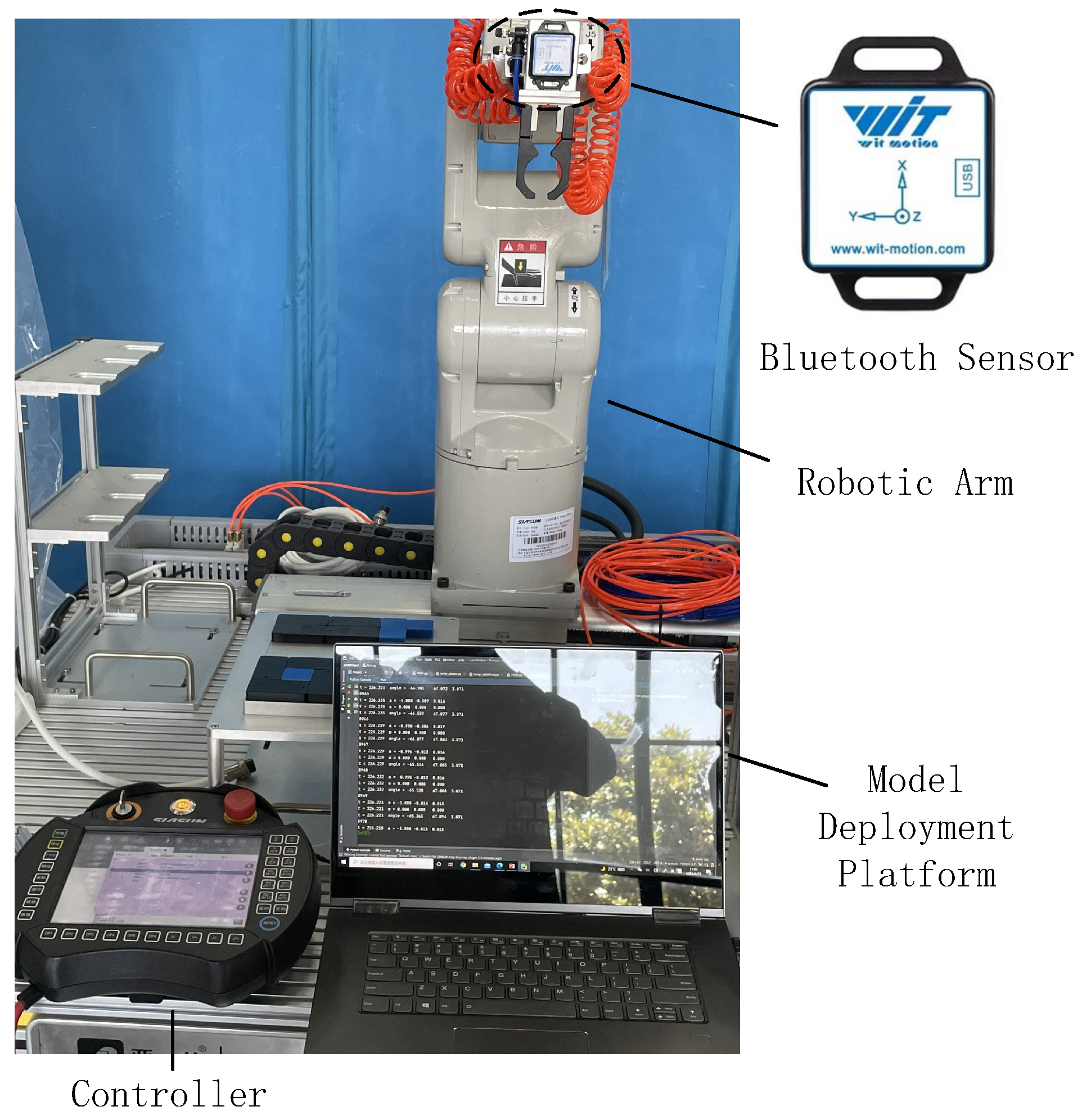
Figure 1 shows the physical experiment platform, which consists of the controller, the robotic arm of SIASUN SR4B, the Bluetooth sensor, and the model deployment platform.

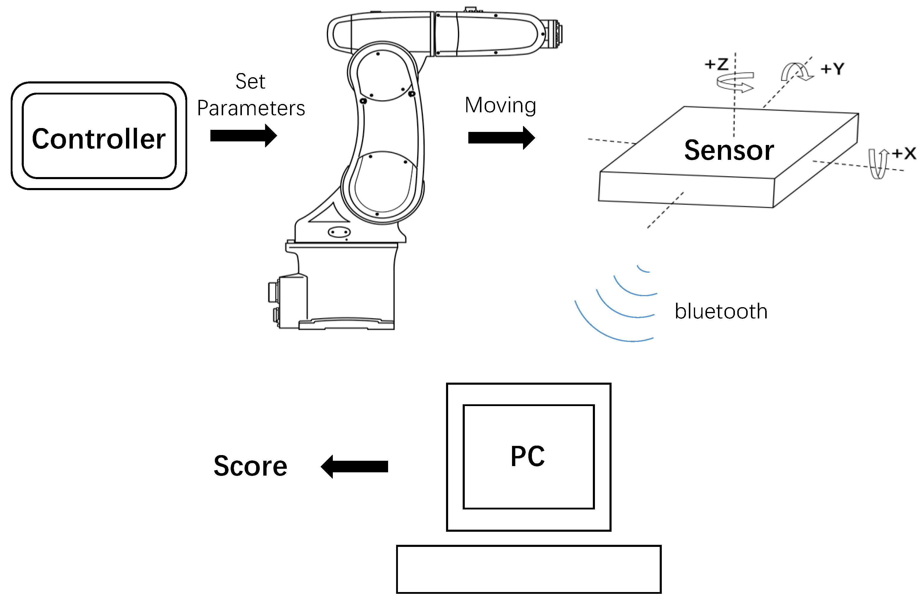
Figure 2 gives the diagram of the stability evaluation system. The controller is used to set dynamic parameters and teach the robot motion process. The scheme in this article is built and tested based on the dataset obtained from the SIASUN six-axis robotic arm SR4B. The inertial measurement method [17] is utilized to obtain signals. The measurement sensor WIT-BWT61CL, which integrates the accelerometer and gyroscope, is attached to the end effector of the manipulator to obtain the displacement, velocity, and acceleration signals in three directions of X, Y, and Z in Cartesian coordinates. Signals are sent to the model deployment platform by Bluetooth, where the scorecard model is built and tested.

The manipulator is controlled by programs, and a single instruction corresponds to a one-step move. Thus, parameters such as velocity (v), acceleration (a), and displacements in commands can make a great difference to the working stability performance of manipulators. Since the research is faced with robot training, the experiments are conducted according to the real work of robots, such as palletizing. The experiments are performed setting v and a varying among 10%, 20%, …, 100% and the moving steps varying among 2–10 steps. A total of 1000 samples containing vibration signals of angle ($\theta$), angular velocity (w), and acceleration (a) in the X, Y, and Z directions are obtained for modeling and testing.

2.2. Stability Labeling

The stability evaluation of the robotic arm includes the overall stability evaluation and the specific scoring. Signals of vibrations including acceleration, velocity, displacement, etc. are considered for index design in the research related to the stability of manipulators. Rigid shock means the velocity is discontinuous, resulting in a huge acceleration. Flexible shock means the discontinuity of acceleration. These two factors are usually considered the cause of instability, which can be obtained by the calculation of acceleration. Thus, acceleration (a) is chosen for the generation of the evaluation index. First of all, the vibration signals are separated into structural vibration components and motion-generated vibration components by the wavelet transform maxima modulus (WTMM) method. Then, the acceleration signal is utilized to design the evaluation index (EI) for overall evaluation. On this basis, the binary classification labels of good or bad for stability are obtained for the samples.

2.2.1. Wavelet Transform Maxima Modulus (WTMM)

The stability of the manipulator can be measured from two aspects. One is the motion characteristics of the manipulator, i.e., the main components of vibration signals. The other is the influence of the mechanical arm structure itself. The vibration components caused by the main motion of the manipulator are characterized by large amplitude, low frequency, and low singularity. On the other hand, the vibration caused by structure deformation has high frequency and small amplitude as well as strong randomness. WTMM is suitable for separating the components with large singularity and is used to separate the two vibration components according to their different properties.

The WTMM was proposed by Mallat [18]. In WTMM, the modulus maxima in each layer are filtered when the corresponding Lipschitz exponent $\alpha$ is less than 0. The remaining modulus maxima are used to reconstruct the filtered signal by the cross-projection method [19]. The Lipschitz exponent is often used to measure the singularity of a function. The signal that is differentiable at a high order at a certain point or interval is smooth in this region and has a small singularity and large $\alpha$. On the contrary, the smaller the $\alpha$, the larger the singularity of the signal. When the signal satisfies Equation (1), the signal is admitted to have a consistent Lipschitz exponent in the interval, where k is an integer and $W_f$ is the wavelet transform modulus maxima of signal x at layer j.

$$\left|W_f\left(2^j,x\right)\right|\le k{2}^{2\alpha }$$

(1)

As shown in Equation (2), the Lipschitz exponent $\alpha$ can be expressed as the logarithm of the ratio of the modulus maxima $W_f$ between different scales j and $j+1$.

$$\alpha ={\log }_2\frac{\left|W_f\left(2^{j+1},x\right)\right|}{\left|W_f\left(2^j,x\right)\right|}$$

(2)

When $\alpha >0$, the maxima increase as j increases. When $\alpha <0$, the maxima decrease as j increases. The maxima do not vary with j when $\alpha =0$.

When it comes to vibration signal analysis of the manipulator, the vibration component brought by the motion itself, denoted as $a_{main}$, has a lower frequency and is smoother. The component caused by structural deformation, denoted as $a_{vib}$, has a higher frequency and stronger singularity. The WTMM is used to separate these two vibration components:

• Perform binary wavelet transform on the signal, select db3 wavelet, and calculate the modulus maximum points of the wavelet coefficient on each scale;
• On the largest scale j, set the threshold of the modulus maximum points, filter out the modulus maximum points below the threshold, and obtain new modulus maxima;
• Starting from the scale $j-2$, filter out the points corresponding to the position where the modulus maximum value is 0 at the higher scale. Repeat until j = 2, and only keep the modulus maxima that are not zero when $j-2$;
• Use the cross-projection method to reconstruct the signal $a_{main}$ with the remaining modulus maximum points; the filtered part is $a_{vib}$.

2.2.2. Evaluation Index (EI)

Based on the vibration signals, we need to design an evaluation index to measure the overall running stability of the robotic arm, where the Jerk and the average power of different vibration components are considered.

• Jerk: As shown in (3), Jerk is defined as the mean absolute value of the derivative of acceleration a in the X, Y, and Z axis directions with the unit of g/s. Jerk indicates how fast the acceleration changes during the movement. Severe acceleration changes harm the stability of the manipulator. The rapidly changing acceleration corresponds to the rapidly changing torque applied to the manipulator, which causes the violent vibration of the arms. Therefore, Jerk and stability should be negatively correlated, and the larger the Jerk, the worse the stability. T is the time of each sample in (3).

  $$Jerk=\frac{1}{T}\sum _{x,y,z}\sum _{t=0}^T\left|\frac{da\left(t\right)}{dt}\right|{\Delta }_t$$

  (3)
• Average Power (AP): AP is defined as the energy of acceleration (a) divided by time and has the dimension of $g^2$. When the energy of the vibration is greater and the time is shorter, it indicates that the vibration is more intensive and severe. Since the signal of a is separated into components of $a_{main}$ and $a_{vib}$, $A{P}_{main}$ and $A{P}_{vib}$ stand for the average power of the corresponding components.

  $$A{P}_{main}=\frac{1}{T}\sum _{x,y,z}\sum _{t=0}^T{\left|a_{main}\left(t\right)\right|}^2{\Delta }_t$$

  (4)

  $$A{P}_{vib}=\frac{1}{T}\sum _{x,y,z}\sum _{t=0}^T{\left|a_{vib}\left(t\right)\right|}^2{\Delta }_t$$

  (5)

The design of the stability evaluation index (EI) comprehensively considers the Jerk and AP as follows:

$$EI=\alpha \times \frac{A{P}_{main}-\overline{A{P}_{main}}}{{\delta }_{A{P}_{main}}}+\beta \times \frac{A{P}_{vib}-\overline{A{P}_{vib}}}{{\delta }_{A{P}_{vib}}}+\gamma \times \frac{Jerk-\overline{Jerk}}{{\delta }_{Jerk}}$$

(6)

where $\overline{A{P}_{main}}$, $\overline{A{P}_{vib}}$, and $\overline{Jerk}$ represent the average value and ${\delta }_{A{P}_{main}}$, ${\delta }_{A{P}_{vib}}$, and ${\delta }_{Jerk}$ are the standard deviations of the corresponding statistics of the samples. $\alpha$, $\beta$, $\gamma$ are weight coefficients, ranging from 0 to 1. Here, they are set default as $\frac{1}{3}$. To sum up, the larger the EI, the worse the motion stability of the manipulator. On the contrary, the smaller the EI, the better the stability.

2.2.3. Stability Labeling

The states of stability among the captured samples are classified into two categories, good or bad, by calculating EI. $\overline{EI}$ is the averaged value among all the 1000 samples, and it is close to 0, representing the average stability level. It is assumed that when the EI of the sample is greater than the average level, it is judged to be unstable, and the label value is set to 1. When the EI of the sample is less than the average level, it is judged to be stable, and the label value is 0, as shown in (7).

$$y=\left\{\begin{array}{ccc}\hfill 1& \hfill & \hfill \mathrm{if}EI>\overline{EI}\\ \hfill 0& \hfill & \hfill \mathrm{if}EI\le \overline{EI}\end{array}\right.$$

(7)

To sum up, the overall stability labels of the vibration samples are obtained based on the proposed scheme, which depends on the raw vibration statistics. Compared with manual labeling, the proposed method is more objective and standardized.

2.3. Scorecard Model

The scorecard model is often used for the risk-level assessment in the field of financial risk control. It is applied to scoring the risk level of medical surgery in [20]. Li et al. [21] established a scorecard model to evaluate the transformer status. In this section, the relevant theories of the scorecard model are introduced into the scene of stability evaluation for robot training, where the specific score of motion staibilty is obtained based on the information extracted from the vibration signals. The process includes feature extraction, binning, WOE transformation, feature selection, logistic regression, and score transformation.

2.3.1. Feature Extraction

In addition to the effects of $Jerk$, $A{P}_{main}$, and $A{P}_{vib}$, there may be other factors embodied in the vibration signals that play a role in the stability scoring for robotic arms. Therefore, more detailed features are extracted from the collected vibration signals for modeling. Statistics are calculated from the acceleration and angular velocity of the collected signals as initial features. The 11 extracted initial features include $\left|\overline{a_{main}}\right|,{\delta }_{a_{main}}$, $\left|\overline{a_{vib}}\right|,{\delta }_{a_{vib}}$, $a_p$, $\left|\overline{w}\right|,{\delta }_w,w_p$ and the aforementioned $A{P}_{main},A{P}_{vib},$ and $Jerk$. The absolute mean value, the standard deviation, and the peak value are defined as Equations (8)–(10), where x is the corresponding variable of $a_{main}$, $a_{vib}$, a, or w.

$$\left|\overline{x}\right|=\frac{1}{N}\sum _{n=1}^N\left|x\left(n\right)\right|$$

(8)

$${\delta }_x=\sqrt{\frac{1}{N-1}\sum _{n=1}^N{\left[x\left(n\right)-\overline{x}\right]}^2}$$

(9)

$$x_p=\max \left|x\left(n\right)\right|$$

(10)

2.3.2. Variable Binning

Variable binning is the piecewise discretization of continuous feature variables. The chi-square binning method is used to bin the continuous features as follows:

• Set the initial discrete intervals of a feature, and calculate the chi-square value of each pair of adjacent intervals. The chi-square value is calculated as (11):

  $$X^2=\sum _{i=1}^n\sum _{j=1}^2\frac{{\left(A_{ij}-E_{ij}\right)}^2}{E_{ij}}$$

  (11)
  $A_{ij}$ represents the number of samples of class j in the ith interval of the feature. $E_{ij}=\frac{N_i}{N}\times C_j$, where N is the total number of samples, $N_i$ represents the number of samples in the ith interval, and $C_j$ is the number of samples of class j in all samples.
• Merge the adjacent intervals if they have similar chi-distributions on the labels; i.e., the chi-square value of the intervals is less than the set threshold.
• Repeat 1 and 2 until the number of bins reaches the set value.

The values of continuous variables change frequently and irregularly, while the small changes may not greatly impact the vibration stability score. Therefore, chi-square binning is performed on the features to convert the continuous values into discrete intervals. When the values of a feature fall in the same interval, the effects on the score are considered to be consistent.

2.3.3. Weight of Evidence (WOE)

WOE is used to measure the influence of each bin interval of the feature variable on the label value, as shown in Equation (12):

$$WO{E}_i=ln\left(\frac{p_{yi}}{p_{ni}}\right)=ln\left(\frac{y_i/y_T}{n_i/n_T}\right)$$

(12)

where i is the ordinal of the bin, $y_i$ is the number of positive samples in the bin, i.e., the unstable samples, $y_T$ is the number of positive samples of all, $n_i$ is the number of negative samples in the bin, i.e., the stable samples, and $n_T$ is the number of negative samples of all. $p_{yi}$ represents the proportion of the positive samples in the i bin to the total positive samples, and $p_{ni}$ is the proportion of the negative samples in the i bin to the total negative samples. WOE indicates the difference between the bin samples and all samples when it comes to the ratio of positive ones and negative ones. Each bin has the value of WOE. The larger the WOE value, the more likely a sample is judged as unstable when the corresponding feature value falls in the bin interval. On the contrary, the smaller the WOE is, the more likely the sample is stable. On the other hand, the large difference in WOE values under different bins indicates that the feature can well tell the label value. In the scorecard model, the feature binning results are converted into WOE.

2.3.4. Feature Selection

With the initial 11 features extracted from vibration data, it is necessary to further filter out the ones that are meaningless to the model. Here, the screening is conducted based on the predictive ability and linear correlation of the features.

Information Value (IV) is used to evaluate the predictive ability of a feature variable to the stability label. Equations are as follows:

$$I{V}_i=\left(\frac{y_i}{y_T}-\frac{n_i}{n_T}\right)\times WO{E}_i$$

(13)

$$IV=\sum _i^{n}I{V}_i$$

(14)

$I{V}_i$ is the information value in the ith bin of the feature variable, and the IV value corresponds to the feature and is the sum of the $I{V}_i$ values of all bins. The larger the IV value, the greater the difference in the WOE values in the bins of the feature; i.e., the stronger the ability to predict the label. Common thresholds for feature screening using IV values are shown in

Table 1. Thresholds of IV.

IV	Predictive Ability
<0.02	None
0.02–0.1	Low
0.1–0.3	Mid
0.3–0.5	High
>0.5	Highest

.

Linear correlation is also considered for feature selection, including the correlation between features and labels as well as the pairwise correlation among features. As (15), the Pearson coefficient is adopted to evaluate the linear correlation of variables. The range of the coefficient is [−1, 1]. A large absolute value of the coefficient means a strong linear correlation between two features.

$$r_{X,Y}=\frac{cov\left(X,Y\right)}{{\delta }_X{\delta }_Y}=\frac{E\left(\left(X-\overline{X}\right)\left(Y-\overline{Y}\right)\right)}{\sqrt{{\sum }_{i=1}^n{\left(X_i-\overline{X}\right)}^2}\sqrt{{\sum }_{i=1}^n{\left(Y_i-\overline{Y}\right)}^2}}$$

(15)

For feature selection, the retained features have large IV values, strong correlations with labels, and weak correlations with each other.

2.3.5. Logistic Regression Model

The logistic regression (LR) model is commonly used in the scorecard model, which is simple, stable and interpretable. The LR model is able to learn the linear relationship between the WOE of features and the logarithm of the unstable probability, and it gives the coefficient of each feature. It is similar to obtaining the scores for each item first and adding them up to obtain the final score.

A logistic regression model is represented as $P\left(y|x\right)$:

$$P\left(y=1|x\right)=\frac{1}{1+e^{-w·x}}$$

(16)

$$P\left(y=0|x\right)=\frac{e^{-w·x}}{1+e^{-w·x}}$$

(17)

where x is the processed input vector $x={\left(x^{\left(1\right)},x^{\left(2\right)},\dots ,x^{\left(n\right)},1\right)}^T$, i.e., the WOE of selected features in this occasion, y is the stability label with the value of 1 or 0, and w is the weight vector $w={\left(w^{\left(1\right)},w^{\left(2\right)},\dots ,w^{\left(n\right)},b\right)}^T$. The positive and negative probabilities are calculated, and the sample is classified into the class with a larger probability value. Odds are defined as the ratio of positive and negative probabilities and are introduced to the scoring model. The equations below show the odds and their logarithm (logit).

$$odds=\frac{p}{1-p}$$

(18)

$$logit\left(p\right)=log\frac{p}{1-p}$$

(19)

where p is the positive probability. (20) can be obtained combining (16)–(19):

$$log\frac{P(y=1|x)}{1-P(y=1|x)}=w·x$$

(20)

where the logit is expressed as a linear function of the input of x.

The process of logistic regression is to find suitable coefficients of w through supervised learning to make the probability value of the sample consistent with the stability label. The maximum likelihood method is used to estimate parameters. Assuming:

$$P\left(y=1|x\right)=\pi \left(x\right),P\left(y=1|x\right)=1-\pi \left(x\right)$$

(21)

The log likelihood function is as follows:

$$\begin{array}{cc}\hfill L\left(w\right)& =\sum _{i=1}^N[y_{i}log\pi \left(x_i\right)+(1-y_i)log(1-\pi \left(x_i\right))]\hfill \\ \hfill & =\sum _{i=1}^N[y_{i}log\frac{\pi \left(x_i\right)}{1-\pi \left(x_i\right)}+log(1-\pi \left(x_i\right))]\hfill \\ \hfill & =\sum _{i=1}^N[y_i(w_i·x_i)-log(1+e^{w·x_i})]\hfill \end{array}$$

(22)

N is the number of samples and $y_i$ is the label value of the ith sample $x_i$. Estimates of coefficients w are obtained by iterative training of the gradient descent and the quasi-Newton method. Thus, the output probability p of the logistic model is obtained, i.e., the instability probability on the occasion of stability evaluation.

2.3.6. Scoring

The corresponding probability output in the scorecard model needs to be further converted into a score, and the logit is introduced into the scoring formula:

$$score=scor{e}_{base}-\frac{pdo}{log2}\times log\left(\frac{p}{1-p}\right)$$

(23)

According to (20), the score can be expressed as:

$$score=scor{e}_{base}-\frac{pdo}{log2}\times w·x$$

(24)

In the equations, $scor{e}_{base}$ and $pdo$ are parameters set to adjust the score range. $scor{e}_{base}$ represents the score when $p=0.5$, i.e., the probabilities are equal between stability and instability. $pdo$ is the reduction of score when $p=\frac{2}{3}$.

Thus, the score of stability evaluation can be expressed as the linear combination of each feature multiplying the corresponding coefficient. It is similar to evaluating the performance of each feature and scoring respectively. The score items include the sub-score of each selected feature and the $scor{e}_{base}$. The final score is the sum of all items, which is the definition of the scorecard. The higher the score, the stronger the stability of the robotic arm.

2.4. Endpoint Localization Method

The vibration signals obtained are usually continuous with multi-steps controlled by several commands. The start and end positions of each step in the vibration signals are defined as the endpoints of the action. Endpoint localization is to identify the start and end positions of a segment in the continuous time-series signal, by which the subsection of the moving process can be obtained and further scored by the scorecard model.

Usually, the wavelet transform (WT) [22] and the double threshold method [23] are utilized to detect the end position of a series of signals. WT can identify the step position, and the double threshold method can detect endpoints through the calculation of the zero-crossing rate and local energy. However, in the case of endpoint localization for manipulator vibration signals, these two methods are susceptible to noise interference. Based on the commonly used methods for endpoints detection, we propose a scheme to automatically identify the endpoints of the vibration signals, including the process of step transformation, wavelet transformation, and localization.

2.4.1. Step Transform

Due to the trajectory generation algorithm of the manipulator motion, the motion process of the manipulator is represented as the shock waveform at the endpoints in the acceleration signal and as the step waveform in the angular velocity signal. With the existence of vibration noise, the shock waveform and the step waveform are irregular. The shock waveform does not only exist at the endpoints, and the angular velocity signal (w) is thus chosen in the endpoint localization process.

Due to the existence of vibration noise, we smooth the w first, as shown in Equation (25).

$$w=\left\{\begin{array}{cc}\hfill 0& \left|w\right|<1\\ \hfill w& \mathrm{else}\end{array}\right.$$

(25)

To detect the front and rear endpoints of the angular velocity ladder waveform, step transformation is performed on the smoothed angular velocity signal as (26). Due to the presence of vibrational noise, multiple step form signals may appear at the endpoints.

$$w=\left\{\begin{array}{cc}\hfill 1& w>0\\ \hfill -1& w<0\\ \hfill 0& \mathrm{else}\end{array}\right.$$

(26)

2.4.2. Wavelet Transform (WT)

After the step transformation, the waveforms of vibration signal w appear as intensive step jumps at endpoints, while they appear as smooth straight lines in the middle of motions. The positions of the step jumps can be easily detected by the wavelet transform.

Wavelet transform is often used for time-frequency analysis of unstable signals and is suitable for the detection of mutation points. Since the collected signal is discrete, discrete wavelet transform (DWT) is utilized here. As shown in Equations (27) and (28), the signal can be decomposed into a set of linear combinations of wavelet series with different scales and displacements by DWT:

$$f\left(t\right)=\sum _k\sum _j{a}_{j,k}{\psi }_{j,k}\left(t\right)$$

(27)

$${\psi }_{j,k}\left(t\right)=2^{-\frac{j}{2}}\psi \left(2^{-j}t-k\right)$$

(28)

where j represents the scale, and k represents the displacement. In the discrete wavelet trans-form, the scale j is a discrete value representing the frequency resolution, and k is the time shift. $a_{j,k}$ is the wavelet coefficient representing the energy of the signal at the corresponding time-frequency point.

On this basis, the Mallat algorithm uses a set of orthogonal wavelet bases to decompose the signal, as shown in Equations (29) and (30).

$$f\left(t\right)=\sum _k{c}_{j_0,k}{\varphi }_{j_0,k}\left(t\right)+\sum _k\sum _j{d}_{j,k}{\psi }_{j,k}\left(t\right)$$

(29)

$$\left\{\begin{array}{ccc}\hfill c_{j_0,k}& =\hfill & \hfill 〈f\left(t\right),{\varphi }_{j_0,k}\left(t\right)〉\\ \hfill d_{j,k}& =\hfill & \hfill 〈f\left(t\right),{\psi }_{j,k}\left(t\right)〉\end{array}\right.$$

(30)

The first term is the approximation of the signal where $c_{j_0,k}$ is the approximation coefficient. The second term contains the detailed information of the signal and $d_{j,k}$ is the detail coefficient of the signal. The coefficient equals the sum of the inner products between the signal and the wavelet bases.

To locate the position of steps, a three-layer discrete wavelet transform based on db wavelet is performed on the processed signal. As shown in Figure 3, the approximate coefficients and detail coefficients are obtained in the decomposition of each layer, and then, the approximate coefficients are further decomposed in the next layer. The step signal is reflected in the high-frequency components after wavelet decomposition, i.e., the detail coefficient. D1 is selected for the later localization analysis, and its frequency band is $[\frac{1}{2},1]$ of the signal frequency.

2.4.3. Localization

After wavelet decomposition, $D_1$ appears as short-length high-frequency noise segments near the endpoints, and the values of $D_1$ are small in the non-endpoint range. The endpoints can be located by identifying the center of each noise segment in $D_1$. A windowed moving average is performed on $D_1$ as (31), which converts the irregular noise segments into peaks. Then, the endpoints can be easily located by identifying the midpoints of peaks in $D_1$.

$$D_1\left(k\right)=\overline{\sum _{k-width}^{k+width}\left|D_1\left(i\right)\right|}$$

(31)

The endpoints positioning process needs to be conducted on the velocity signals of the X, Y, and Z axes, respectively. Considering the positioning results in the three directions, including the number of positioning points and the width of the wave crest, the final positions of the endpoints are obtained.

With the endpoint localization method, vibration signals of the moving process can be cut into pieces for each action, which makes it possible to score parts of the robotic arm movements.

3. Results

Physical experiments are conducted based on the SR4B 6-axis robot to verify the effectiveness of the proposed scheme for the stability evaluation of robotic arms. The process of EI design and scorecard establishment are presented, proving the reasonability of the evaluation scheme. Examples are tested to show the results of endpoint localization methods as well.

3.1. Labeling

The overall stability index is designed and statistics are calculated on the samples. The samples with $EI>0$ are labeled as unstable, while the others are labeled as stable. The distribution of index on the samples is as

Table 2. Statistics of evaltion index on the samples.

Label	Number	$\overline{\mathit{EI}}$	$\overline{{\mathit{AP}}_{\mathit{main}}}\left({\mathit{g}}^2\right)$	$\overline{{\mathit{AP}}_{\mathit{vib}}}\left({\mathit{g}}^2\right)$	$\overline{\mathit{Jerk}}\left(\mathit{g}\right)$
Unstable	400	0.7135	0.4675	0.0025	0.0937
Stable	600	−0.5153	0.0364	0.0007	0.0468

.

$\alpha$, $\beta$, and $\gamma$ are set to $\frac{1}{3}$ in the calculation. The stability label of the samples is decided based on the index distribution in the dataset. Obviously, the $\overline{EI}$ of the samples with an instability label is larger than that of the stable samples. Compared with artificial evaluation, the proposed scheme of labeling is based on the statistical results of the evaluation index on the actual vibration data. What is more, it is only used for two-category labeling, which has a higher fault tolerance rate and strong robustness.

3.2. Scorecard

To establish the scorecard for stability evaluation of robotic arms, 11 initial features are extracted, binned, and transformed into WOE, including $\left|\overline{a_{main}}\right|$, ${\delta }_{a_{main}}$, $\left|\overline{a_{vib}}\right|$, ${\delta }_{a_{vib}}$, $a_p$, $\left|\overline{w}\right|$, ${\delta }_w$, $w_p$, $A{P}_{main}$, $A{P}_{vib}$, and $Jerk$. The linear correlation coefficients and IV of the features are calculated for feature selection.

Figure 4 and

Table 3. Variable linear correlation coefficient.

	$\left|\overline{{\mathit{a}}_{\mathit{main}}}\right|$	${\mathit{\delta }}_{{\mathit{a}}_{\mathit{main}}}$	$\left|\overline{{\mathit{a}}_{\mathit{vib}}}\right|$	${\mathit{\delta }}_{{\mathit{a}}_{\mathit{vib}}}$	${\mathit{a}}_{\mathit{p}}$	$\left|\overline{\mathit{w}}\right|$	${\mathit{\delta }}_{\mathit{w}}$	${\mathit{w}}_{\mathit{p}}$	${\mathit{AP}}_{\mathit{main}}$	${\mathit{AP}}_{\mathit{vib}}$	$\mathit{jerk}$	$\mathit{Label}$
$\left|\overline{a_{main}}\right|$	1.000	0.800	0.585	0.570	0.643	0.371	0.538	0.499	0.768	0.545	0.387	0.502
${\delta }_{a_{main}}$	0.800	1.000	0.663	0.677	0.773	0.370	0.625	0.448	0.744	0.603	0.500	0.582
$\left|\overline{a_{vib}}\right|$	0.585	0.663	1.000	0.841	0.640	0.388	0.368	0.277	0.428	0.668	0.669	0.714
${\delta }_{a_{vib}}$	0.570	0.677	0.841	1.000	0.773	0.454	0.358	0.275	0.456	0.696	0.577	0.752
$a_p$	0.643	0.773	0.640	0.773	1.000	0.335	0.433	0.369	0.678	0.749	0.383	0.585
$\left|\overline{w}\right|$	0.371	0.370	0.388	0.454	0.335	1.000	0.488	0.254	0.242	0.266	0.266	0.376
${\delta }_w$	0.538	0.625	0.368	0.358	0.433	0.488	1.000	0.639	0.565	0.328	0.284	0.348
$w_p$	0.499	0.448	0.277	0.275	0.369	0.254	0.639	1.000	0.510	0.230	0.102	0.241
$A{P}_{main}$	0.768	0.744	0.428	0.456	0.678	0.242	0.565	0.510	1.000	0.515	0.162	0.331
$A{P}_{vib}$	0.545	0.603	0.668	0.696	0.749	0.266	0.328	0.230	0.515	1.000	0.412	0.603
$jerk$	0.387	0.500	0.669	0.577	0.383	0.266	0.284	0.102	0.162	0.412	1.000	0.653
$label$	0.502	0.582	0.714	0.752	0.585	0.376	0.348	0.241	0.331	0.603	0.653	1.000

show the linear relationship among the original features as well as the label. The threshold of the linear correlation coefficient is set to avoid multicollinearity between features and ensure the correlation between features and the label. The linear correlation value between any two selected features is less than 0.7. The correlation between each feature and the label is greater than 0.3.

Table 4. IV of features.

$\left|\overline{{\mathit{a}}_{\mathit{main}}}\right|$	${\mathit{\delta }}_{{\mathit{a}}_{\mathit{main}}}$	$\left|\overline{{\mathit{a}}_{\mathit{vib}}}\right|$	${\mathit{\delta }}_{{\mathit{a}}_{\mathit{vib}}}$	${\mathit{a}}_{\mathit{p}}$	$\left|\overline{\mathit{w}}\right|$	${\mathit{\delta }}_{\mathit{w}}$	${\mathit{w}}_{\mathit{p}}$	${\mathit{AP}}_{\mathit{main}}$	${\mathit{AP}}_{\mathit{vib}}$	$\mathit{jerk}$
0.676	0.727	0.845	0.872	0.611	0.007	0.549	0.499	0.645	0.892	0.831

shows the information values of these original variables, representing the ability of each feature to distinguish the stability of the sample. Empirically, the IV threshold for selected features is set to 0.2.

Setting the thresholds of IV and linear correlation coefficients, $\left|\overline{a_{main}}\right|,{\delta }_{a_{main}},a_p,{\delta }_w,$ and $jerk$ are selected as features for scoring. The selected features are used for logistic modeling, with 722 samples as training datasets and the other ones as test datasets. The number of logistic regression iterations is 35, obtaining the logistic regression coefficients, as shown in

Table 5. Coefficients of logistic regression model.

$\left|\overline{{\mathit{a}}_{\mathit{main}}}\right|$	${\mathit{\delta }}_{{\mathit{a}}_{\mathit{main}}}$	${\mathit{a}}_{\mathit{p}}$	${\mathit{\delta }}_{\mathit{w}}$	$\mathit{jerk}$	b
0.237957	0.405033	0.917208	0.117351	1.257588	−0.578872

, where b is the bias term.

Setting the threshold of the model as 0.5, we have the accuracy of 96.4% on the binary classification of the samples on the test dataset. Furthermore, the output probability is converted to scores of stability. The scorecard is obtained as shown in

Table 6. Scorecard.

Feature	Bin	WOE	Item Score
$\left|\overline{a_{main}}\right|$	[−inf, 0.0462) [0.0462, 0.0544) [0.0544, 0.0628) [0.0628, 0.0724) [0.0724, 0.0857) [0.0857, inf)	−1.3793 −1.9877 −1.05 0.2766 1.4051 1.8040	0.4735 0.6824 0.3605 −0.0949 −0.4823 −0.6193
${\delta }_{a_{main}}$	[−inf, 0.0546) [0.0546, 0.0671) [0.0671, 0.0853) [0.0853, 0.1046) [0.1046, 0.1332) [0.1332, inf)	−2.7498 −1.5334 −0.4630 0.8055 0.0122 3.4771	1.6068 0.8960 0.2705 −0.4706 −0.0071 −2.0318
$a_p$	[−inf, 0.2964) [0.2964, 0.4102) [0.4102, 0.5513) [0.5513, 0.7241) [0.7241, 0.9658) [0.9658, inf)	−1.5581 −1.9877 −0.3622 0.4506 0.8977 1.5492	2.0618 2.6302 0.4793 −0.5963 −1.1879 −2.0501
${\delta }_w$	[−inf, 4.4327) [4.4327, 10.225) [10.225, inf)	0.3421 −1.1944 0.6013	−0.0579 0.2022 −0.1018
$jerk$	[−inf, 0.0368) [0.0368, 0.0485) [0.0485, 0.0616) [0.0616, 0.0781) [0.0781, 0.0974) [0.0974, inf)	−10 −10 −1.9877 −0.0781 4.1703 10	18.1431 18.1431 3.6063 0.1418 −7.5662 −18.1431

.

The table includes the binning results of the feature variables, the WOE code of each bin, and the corresponding single item score, which equals $-\frac{w\left(i\right)x\left(i\right)pdo}{log\left(2\right)}$, as discussed in (24). The parameters of the score model are set as $Scor{e}_{base}=75$ and $pdo=1$, which guarantees the score range of 0–100. With the scorecard, we can obtain the single item score by finding the bin of the corresponding feature. The stability score equals the sum of all item scores, adding the $Scor{e}_{base}$ and the bias item.

$$score=scor{e}_{base}-\frac{pdo}{log2}\times \mathrm{b}+\sum _{items}Scor{e}_{item}$$

(32)

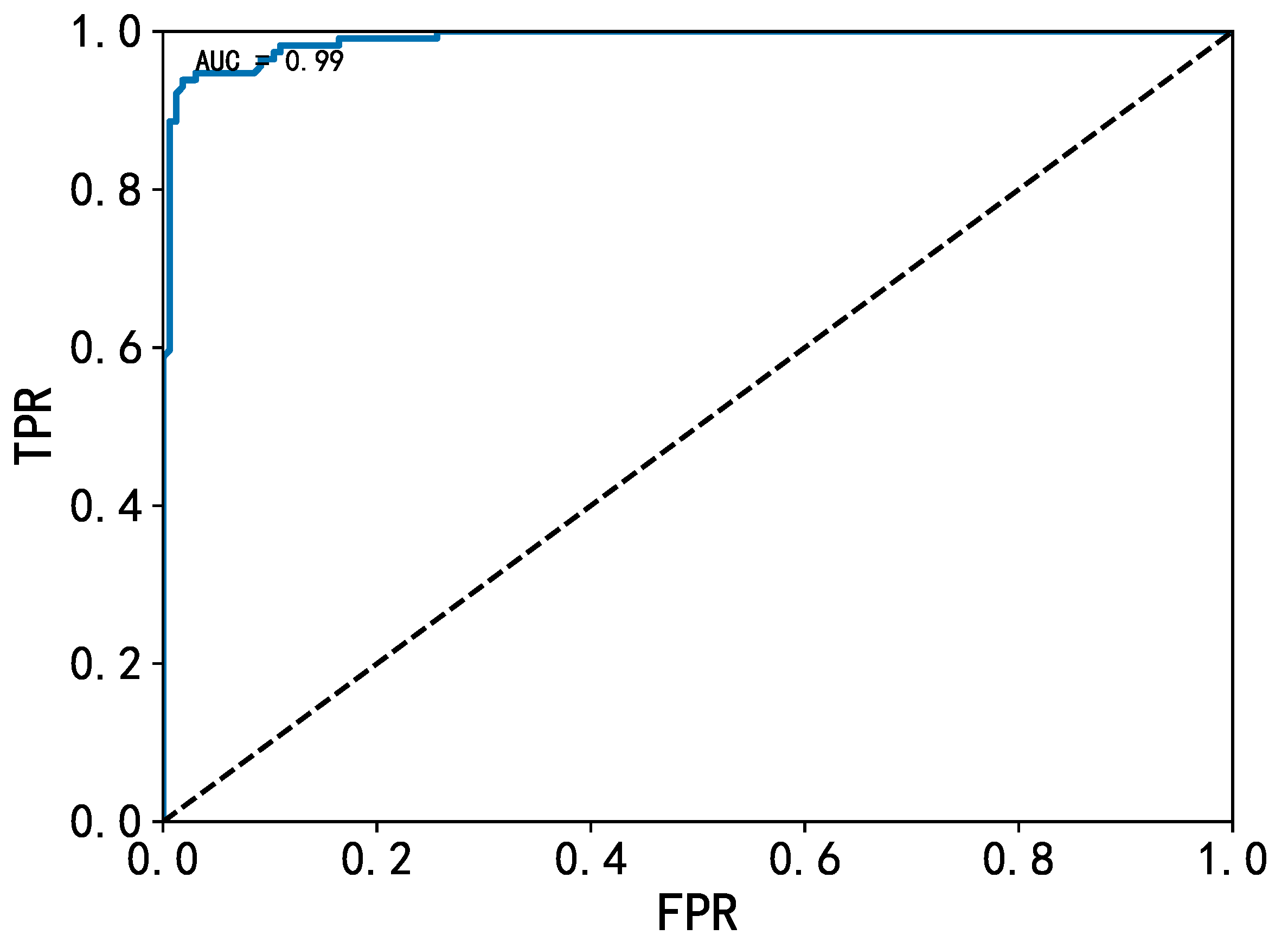
KS and ROC curves are utilized to display the performance of the scorecard model, as shown in Figure 5 and Figure 6.

The KS curve divides the scores into 10 groups from low to high, and it plots the cumulative ratio of positive and negative samples, respectively. Obviously, in the low score groups, the number of unstable samples increases rapidly, while the stable samples are almost 0%. In the high score groups, the number of stable samples increases rapidly, while the unstable samples hardly increase. $KS=0.914$ indicates that the scoring model has a strong ability to discriminate whether the sample is stable or not.

The ROC curve reflects the relationship between the true positive rate and the false positive rate when the corresponding sample is judged to be unstable as the score increases. AUC = 0.99 means that the model is 99% confident that the high score example is stable.

The scoring results of the scorecard model are shown in

Table 7. Feature statistics for score segments.

	(50, 60)	(60, 70)	(70, 80)	(80, 90)	(90, 100)
$\left|\overline{a_{main}}\right|$	0.0902	0.0745	0.0685	0.0555	0.0503
${\delta }_{a_{main}}$	0.1385	0.1109	0.1006	0.0672	0.0553
$\left|\overline{a_{vib}}\right|$	0.0193	0.0147	0.01153	0.0099	0.0066
${\delta }_{a_{vib}}$	0.0291	0.0240	0.0193	0.0161	0.0104
$a_p$	0.9091	0.7803	0.7241	0.4493	0.3326
$\left|\overline{w}\right|$	5.1312	4.8916	4.7796	4.7771	2.7194
${\delta }_w$	10.0246	8.2129	7.6831	7.6668	4.4152
$w_p$	66.7387	52.7907	48.0674	41.3878	31.3652
$A{P}_{main}$	0.07504	0.0548	0.0501	0.0272	0.0162
$A{P}_{vib}$	0.0028	0.0019	0.0012	0.0009	0.0003
$jerk$	0.1160	0.0882	0.0655	0.0533	0.0350

, where the stability scores of the test samples are divided into five groups. The average values in each group are calculated for 11 original features. Each statistic has its actual physical meaning and reflects the stability of the vibration signal. The results show that the mean value of each feature decreases as the score goes from low to high. The scorecard results are consistent with real vibration performance. A higher score indicates that the model considers the stability of samples to be better, and the corresponding actual vibration is smaller.

3.3. Endpoints Localization

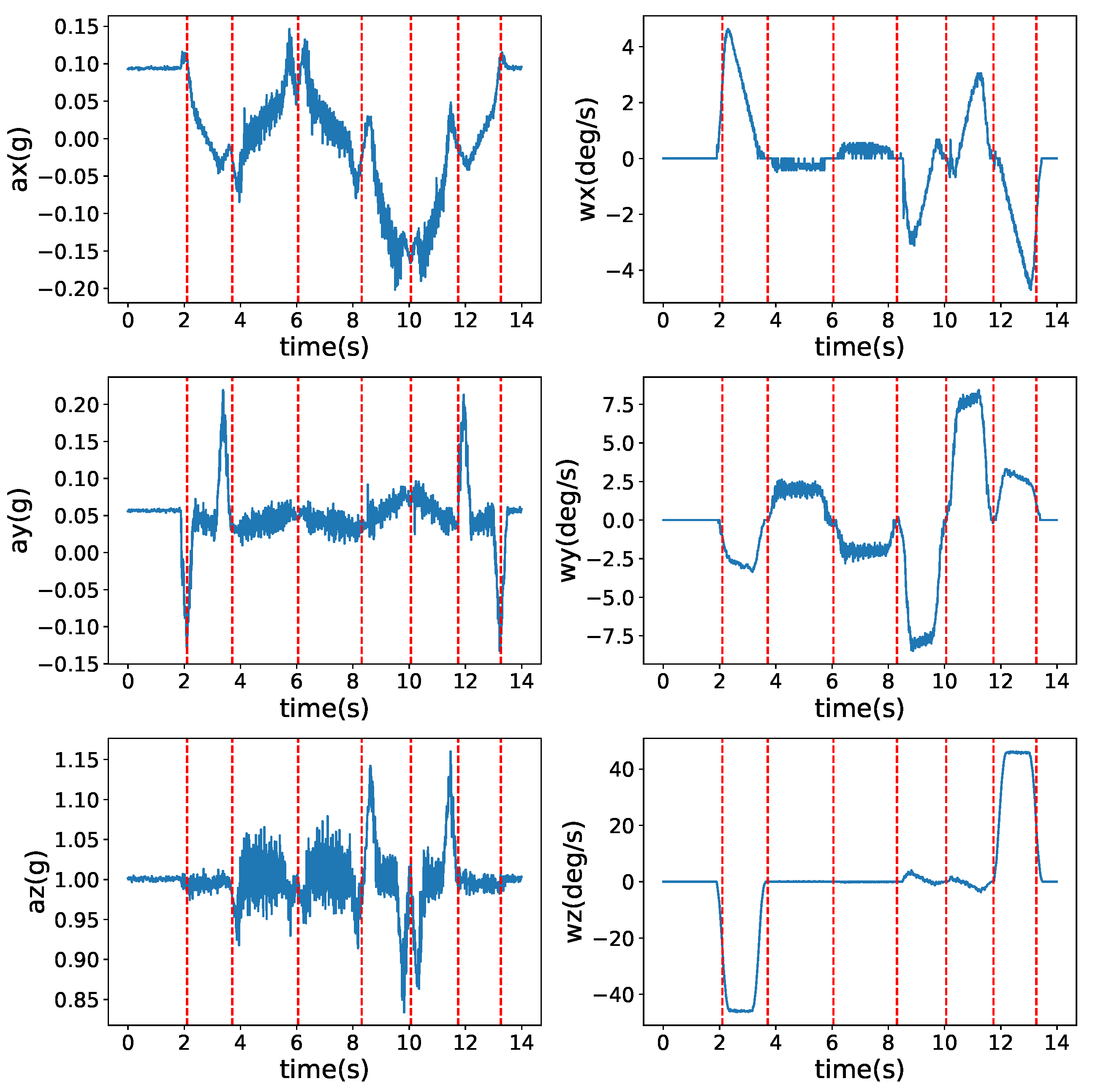
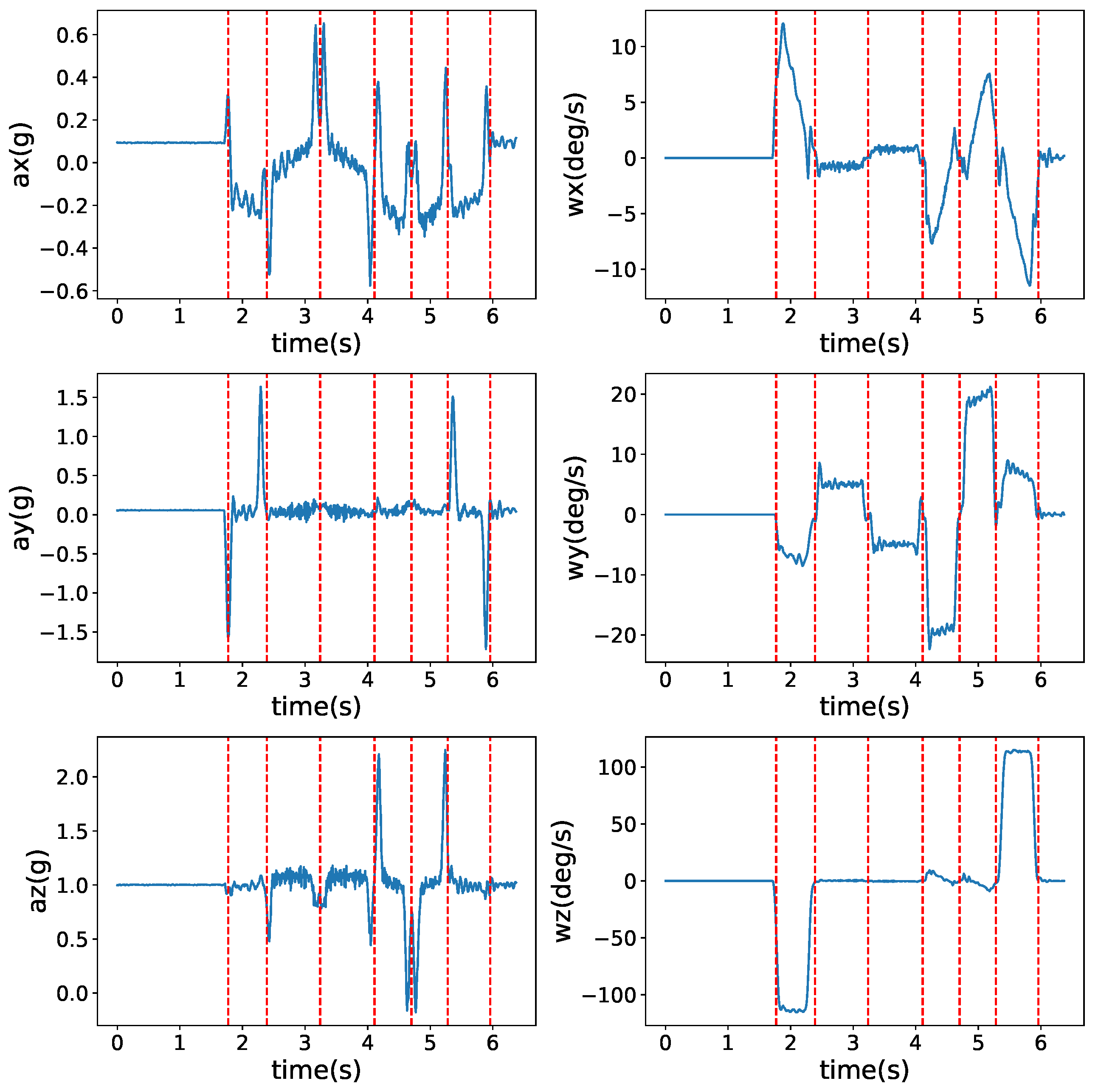
Based on the methods discussed before, the vibration signals of the manipulator can be divided into segments of single actions, which makes it possible to score parts of the moving process. Commonly, a single instruction controls the single-step action of the robotic arm. Examples are given to illustrate the effect of endpoints localization, as shown in Figure 7 and Figure 8. The robot is asked to complete the palletizing task with different set parameters.

These two examples are the signals collected from the six-step movement of the robotic arm at different set speeds and accelerations. The proposed scheme can well identify the locations of endpoints, and the parts of the vibration signals corresponding to the selected actions can be easily obtained and further scored.

4. Discussion

EI is designed and calculated according to vibration signal samples. The average value of EI over the samples is used to judge the stability label. Samples are labeled and statistics are shown in Table 2, which gives the vibration performance of different labeled samples. Consistent with the actual situation, stable samples have lower values of average power and jerk than those of the samples with instability labels.

Figure 4 and Table 3 and Table 4 are used for feature selection in the scorecard model, where the value in Figure 4 and Table 3 means correlation strength, and the IV value in Table 4 indicates the ability to assess stability. Five features are selected for score modeling, and the logistic regression coefficients are demonstrated in Table 5, which can be further used to calculate the item scores. Table 6 gives the scorecard, and the stability score may be obtained by finding the group position of features in the scorecard for each sample. From the scorecard, we can find significant features of $jerk$ and $a_p$, which make a great difference to the score. Figure 5 and Figure 6 prove the reasonability of the scorecard model; the score obtained by the model can sufficiently identify stable and unstable samples. Table 7 displays the statistics of features according to the score groups.

The test of the endpoints localization method gives the examples of vibration sequence segmentation as shown in Figure 7 and Figure 8, in which the continuous signal is divided by steps. The localization method can well identify the positions of endpoints. By applying the proposed scheme, the samples can be segmented automatically. The methods may be applied in situations where the information contained in each action segment can be analyzed and parts of the moving process can be scored.

In summary, the results prove the reliability and objectivity of the scorecard model for the stability evaluation of robotic arms. Usually, in robot training, the teachers give the score according to the robots’ working performance by their empirical data, which are subjective and random. Compared with the common artificial scoring, the proposed scheme has strict mathematical and statistical deduction as theoretical support, which is more objective.

Future works may be investigated in the following aspects:

• The research of this paper is based on the SIASUN SR4B experimental platform for data acquisition and verification. The proposed method may be applied to a variety of robotic arms, but due to the influence of actual experimental conditions, no more experiments have been carried out. Therefore, in the follow-up work, the method can be verified by combining different types of robot platforms, including different degrees of freedom manipulators, parallel manipulators, etc.;
• The method proposed in this paper is based on statistics and machine learning models. With the increase of data volume, the performance may improve.

5. Conclusions

A scorecard model is proposed in this work for the stability evaluation of robotic arms for robot training. Experiments are conducted on the SIASUN 6-axis robotic arm, and over 1000 samples of vibration signals are obtained for modeling. The evaluation index is designed and calculated to decide the stability label of each sample. The results indicate that stable samples are smaller than unstable ones on the index statistics, which is consistent with the physical phenomenon. The scorecard is obtained to score the stability performance of manipulators. Stability scores of vibration samples can be obtained by calculating features and querying the scorecard. The score statistics show the reasonableness of the performance of different score segments on the characteristics. By applying the scorecard model to robot training, students can obtain feedback on their own operations based on the scores and make adjustments to their operations. The endpoints localization method may successfully split the motion and can be used to dig out detailed information of each step motion. The proposed scheme is advantageous in terms of its strong adaptability for different robotic arms, as well as its reasonability and objectivity. It may be applicable to solve more practical problems, such as quality inspection, operation training assessment, and performance evaluation for robotic arms.