1. Introduction
The outbreak of coronavirus has made colleges and universities fully aware of the importance of information-based teaching [
1,
2,
3]. A school’s traditional theory combined with an experimental teaching mode is very resource-intensive and can no longer meet the learning needs of students. Only the integration of traditional teaching and informatization can ensure higher teaching quality [
4,
5,
6]. As a professional course that analyzes the fundamental laws and application principles of various electromagnetic phenomena, electromagnetic field theory places high demands on students’ understanding and cognition, and has always been a difficult point for students to learn. A large number of difficult-to-understand formulas greatly hinder students’ understanding and the understanding of abstract objective concepts [
7,
8,
9].
With the gradual maturity of finite element technology, different forms of electromagnetic fields can be realized through corresponding finite element calculations. The electromagnetic field that was originally invisible and intangible can be expressed in the form of a field diagram. This kind of visual teaching that actively adopts the means of modern educational technology can cultivate students’ interest in learning, enrich the teaching content, greatly improve teaching efficiency, and bring the teaching to a new level. However, teaching based on finite element theory is still a computationally expensive process [
10,
11,
12].
On the other hand, with the rapid development of computer technology, research in fields such as machine learning and neural networks has grown rapidly. This research has been gradually applied in the power industry towards problems such as load forecasting, power forecasting of power plants, power grid fault diagnosis and so on [
13,
14,
15]. In terms of magnetic field calculation, Reference [
16] proposed a three-dimensional finite element neural network calculation model and established a magnetic field analysis model based on a finite element neural network. The network did not need to be trained, and iteratively corrected weights from the hidden layer to the output layer to obtain the magnetic scalar potential distribution. Using the Hopfield neural network algorithm, the experts A.A. Adly et al. proposed an automatic integral equation method with which two-dimensional field calculations could be performed in nonlinear magnetic media. They investigated further, using a coupled three-node Hopfield neural network to model interacting magnetized subregions. Their study monitored the local magnetization curves tracked in electromagnetic devices to estimate the evaluation of local hysteresis losses [
17,
18].
Based on the above research on electromagnetic field teaching, a magnetic field visualization teaching method based on finite element theory and neural network is proposed in this paper. Basic data are provided through a certain number of finite element calculations, after which reliable models are built through artificial intelligence methods. On this basis, the model is quickly calculated. In this paper, a magnetic field was used as an example to conduct research based on the above ideas. Firstly, the finite element method was applied to calculate the magnetic field of the magnetic core inductance. Then the neural network method was used to learn the finite element data set and train the model. After training, the results of the magnetic field were predicted by changing the input parameters. By comparing the finite element calculation results with the neural network calculation results, we found that this method improved the computational efficiency and quickly and accurately predicted the coil magnetic field under the given conditions. On this basis, this method can also be extended and applied to other research on magnetic field teaching.
2. Construction of Finite Element and Neural Network Models
The main purpose of magnetic field finite element calculation is to establish a data set for machine learning. After a reliable and stable neural network model is established, when similar magnetic field problems are encountered in classroom teaching, the neural network model can be directly used for calculation.
2.1. Finite Element Modeling Principles
When calculating the magnetic field, the model is regarded as a steady-state field and the displacement current is ignored. At this time, the Maxwell equations are satisfied:
In the formula, H is the magnetic field strength (A/m), J is the current density (A/m2), and B is the magnetic induction intensity, also known as the magnetic flux density (T).
There are constitutive equations in the medium:
where
μ0 and
μr are the vacuum permeability and relative permeability, respectively.
The vector magnetic potential
A is introduced so that
A satisfies:
The boundary conditions in the air domain are expressed as:
where
n is the outer normal unit vector of the conductor surface in the eddy current region.
In addition, the current density also satisfies the equation:
where
Je is the source current density;
N is the number of turns of the winding coil;
Vcoil is the voltage excitation applied on the winding;
Rcoil is the winding resistance;
ecoil is the direction vector of the current density at each point of the current-carrying coil; and
S is the winding coil cross-sectional area.
The simultaneous equation to obtain the relationship between the vector magnetic potential
A and the source current density
Je is:
Since the inductor parameters are known, the core vector magnetic potential A and the magnetic flux density B can be solved together with Equation (3) to complete the calculation of the magnetic field.
2.2. Neural Network Model
The artificial neural network is a parallel, distributed processing structure composed of processing units interconnected with undirected signal channels called connections. These processing units have local memory and can perform local operations that depend solely on the current value of all input signals that arrive at the processing unit via the input link as well as the value stored in the processing unit’s local memory. Each processing unit has a single output connection, and the output signal can be any desired mathematical model. There are many kinds of neural networks, such as radial basis neural networks, Hopfield networks, competitive neural networks, and back-propagation networks [
19,
20,
21].
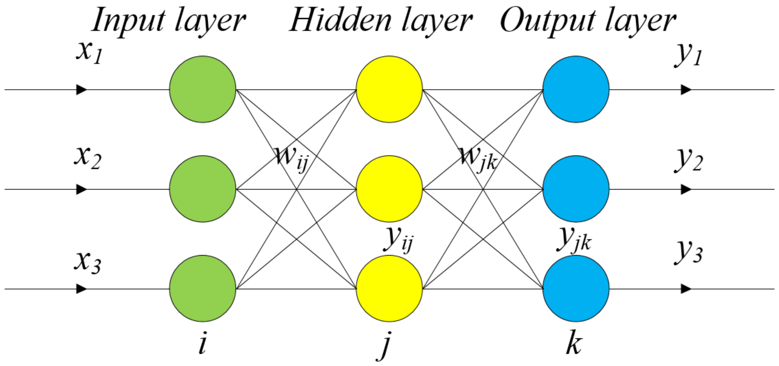
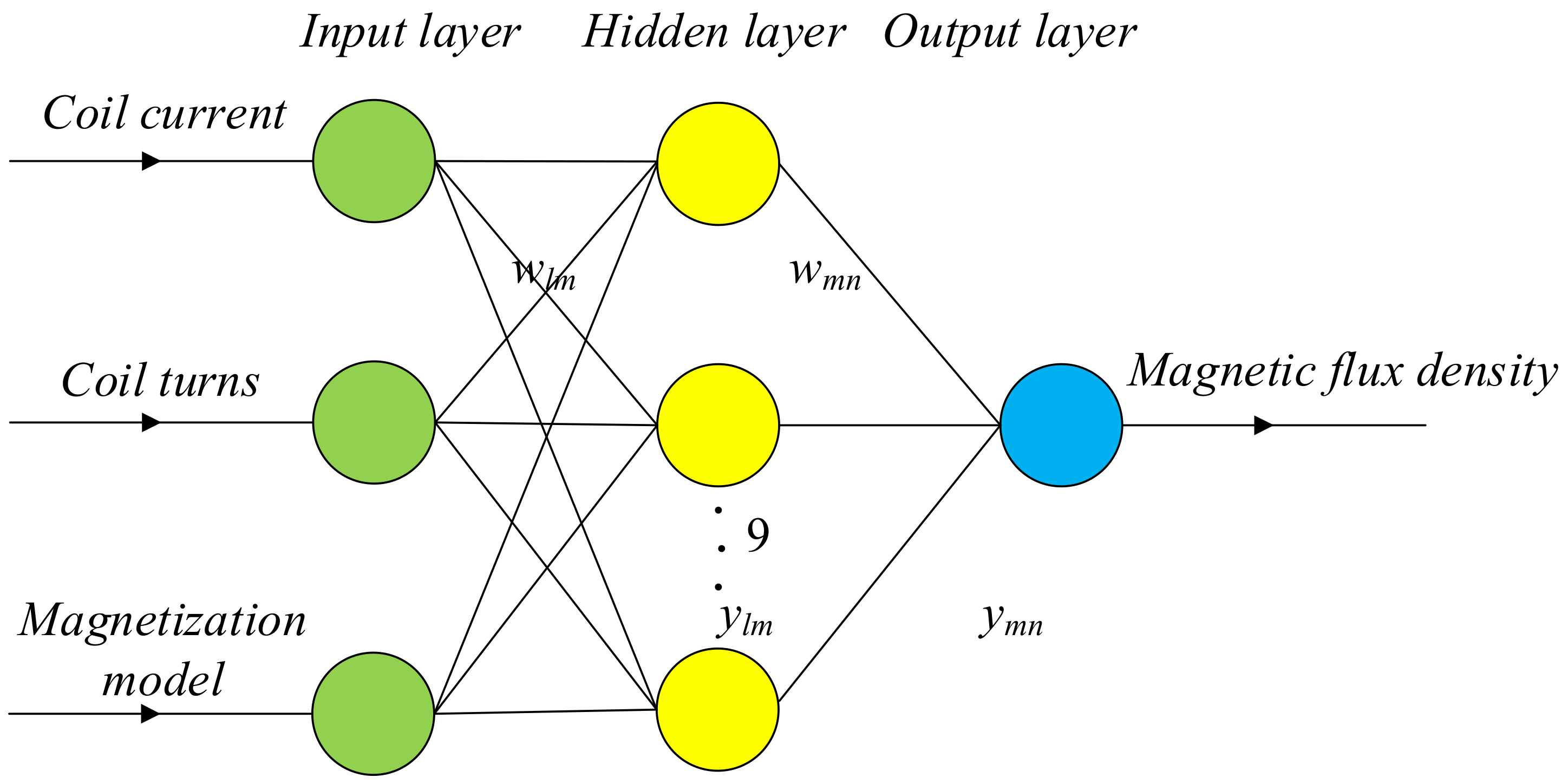
The neural network is a typical multi-layer feedforward (usually three-layer) artificial neural network. Structurally, it consists of input, hidden, and output layers with nodes in each layer. Adjacent layer nodes are connected by weights, but the nodes in each layer are independent of each other. Theoretically, it has been proven that a neural network with a single hidden layer can approximate any nonlinear function with arbitrary precision [
22,
23,
24]. In practical applications, the neural network with a single hidden layer can also meet the needs of calculation well. The structure diagram of the neural network is shown in
Figure 1:
In the figure,
xn is the input variable;
i,
j, and
k are the number of nodes in the input layer, hidden layer, and output layer, respectively;
wij and
wjk are the connection weights between layers; and
yij and
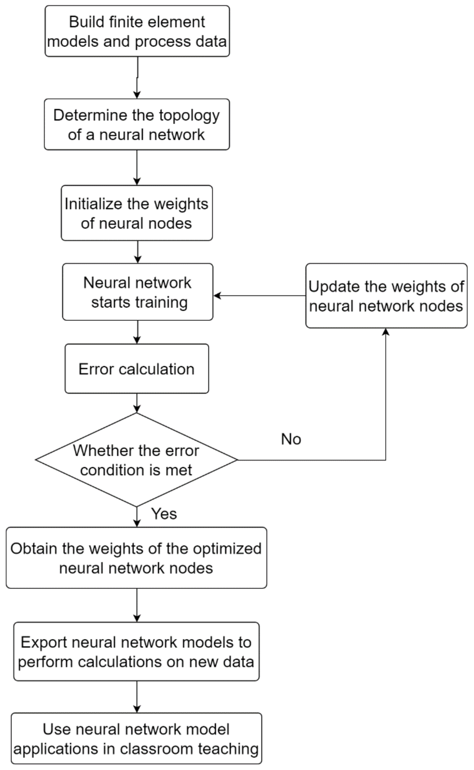
yjk are the output value of the hidden layer and the output value of the output layer, respectively. The flow of the operation process is shown in
Figure 2:
The learning process of the neural network algorithm consists of forward propagation and back-propagation. In the forward propagation process, the input signal of the learning sample is first sent to the input layer. Then it is transmitted to the output layer through the hidden layer, and the corresponding predicted value is output after the calculation of the output layer. When the error between the predicted value and the real value does not meet the preset target accuracy requirements, the network turns to back-propagation. The network feedbacks the error information from the output layer to the input layer by layer, and adjust the weights and thresholds between the layers. Through repeated loop iterations, the error between the output value of the network and the expected output value of the sample is gradually reduced until the set number of loops or accuracy requirements are met. At this point, the learning process of the network ends, and the optimized weights and thresholds are obtained. Then, based on the internal relationship, the input information of the unknown sample is extracted, and the mapping of the unknown sample can be obtained.
In this paper, the iron core material was an isotropic linear material. Additionally, the final magnetic field cloud map B was related to the coil current, the number of coil turns and the magnetization model. As shown in
Table 1, three input quantities were used for the research.
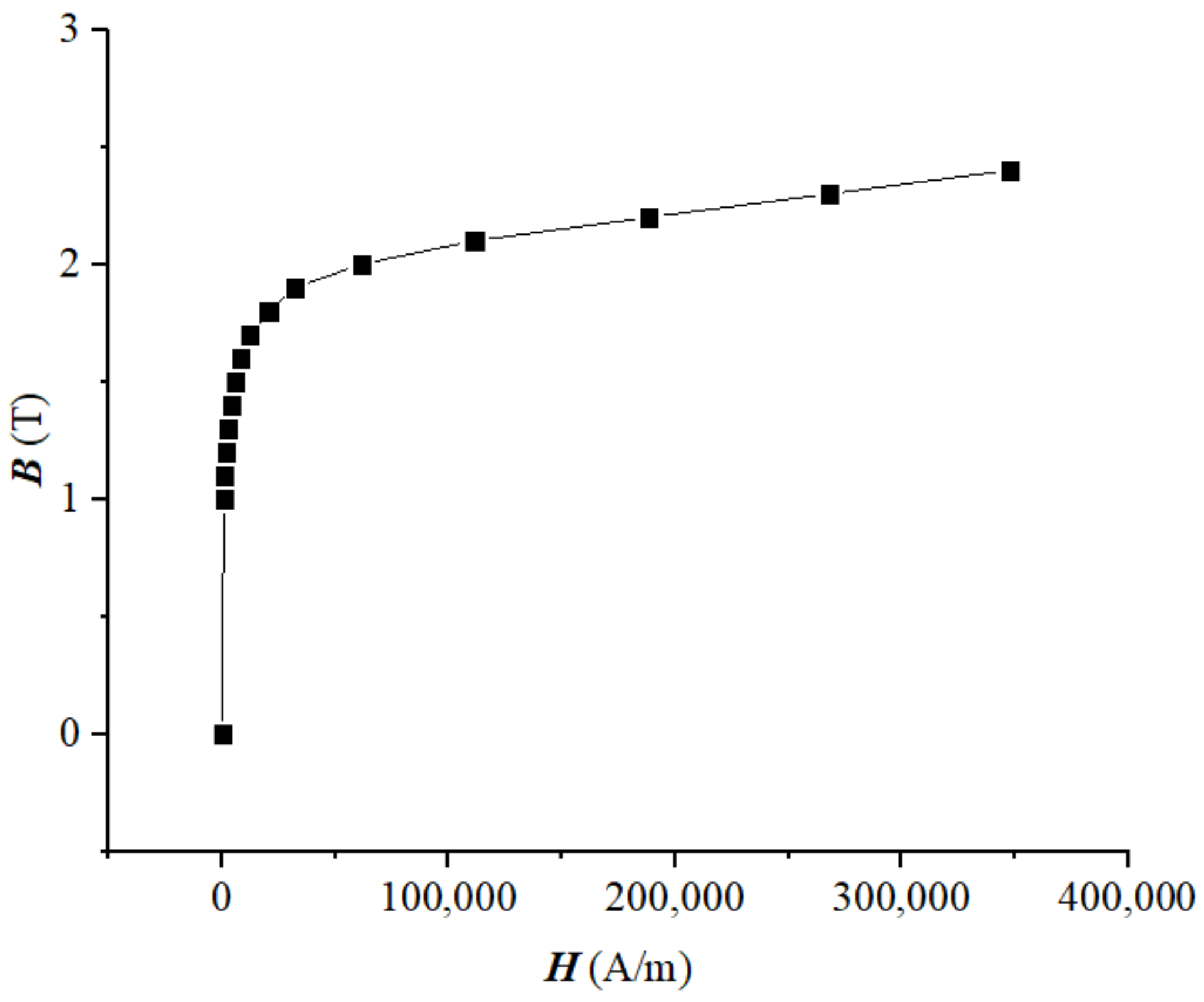
The study considered two magnetization models. The relative permeability was used for the linear material, and the
B-
H curve wa used for nonlinear material. The
B-
H curve for nonlinear material is shown in
Figure 3.
The specific structure of the neural network model in this study is shown in
Figure 4. The number of hidden layer nodes was determined by the empirical formula:
, where a is a constant between 1 and 10. Through experimental comparison, we determined that there were nine hidden layers.
3. Construction and Application of Magnetic Field Visualization Teaching Platform
The time required to calculate the magnetic field of the core inductance using the finite element method was about 12 s. The neural network method was used to learn 100,000 sets of data, and the model obtained from the training was used to predict the magnetic field of the magnetic core inductance; the time required was about 0.07 s. Compared with the finite element method, the calculation time of the magnetic field distribution was decreased by about 170 times through the neural network method. In terms of calculation speed, the neural network model has obvious advantages compared with finite element calculation.
3.1. Magnetic Field Calculation Based on Finite Element Principle
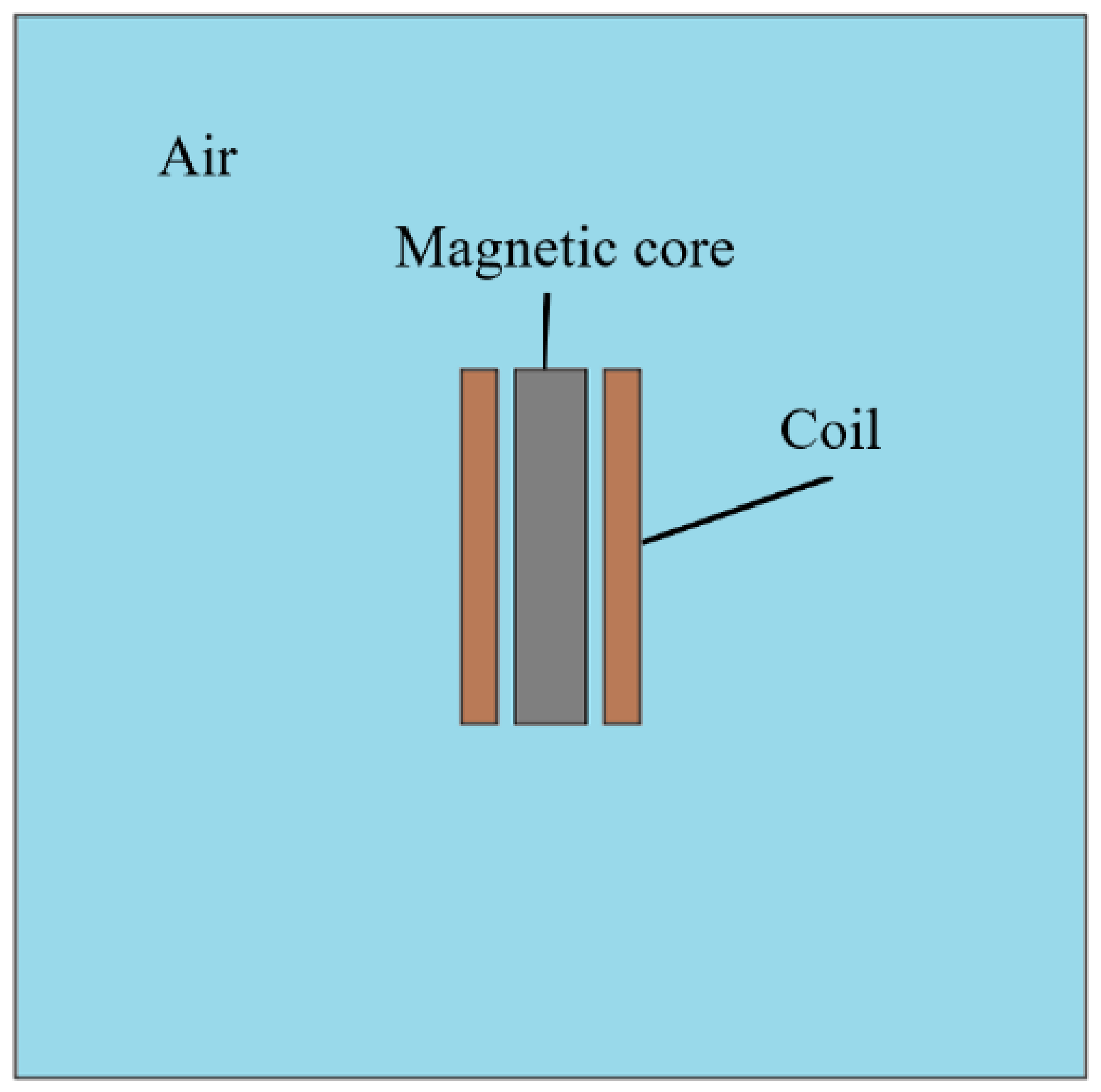
The magnetic core model used in the finite element calculation was a regular rectangle with a shape of 20 mm × 100 mm, and the coils on both sides were a regular rectangle with a shape of 10 mm × 100 mm, which was wound on the magnetic core. The core model of the inductor with the magnetic core is shown in
Figure 5.
The magnetic field parameter settings were: the relative permittivity of the core, winding, and air domain were 1, and the relative permeability of the winding and the air domain were 1.
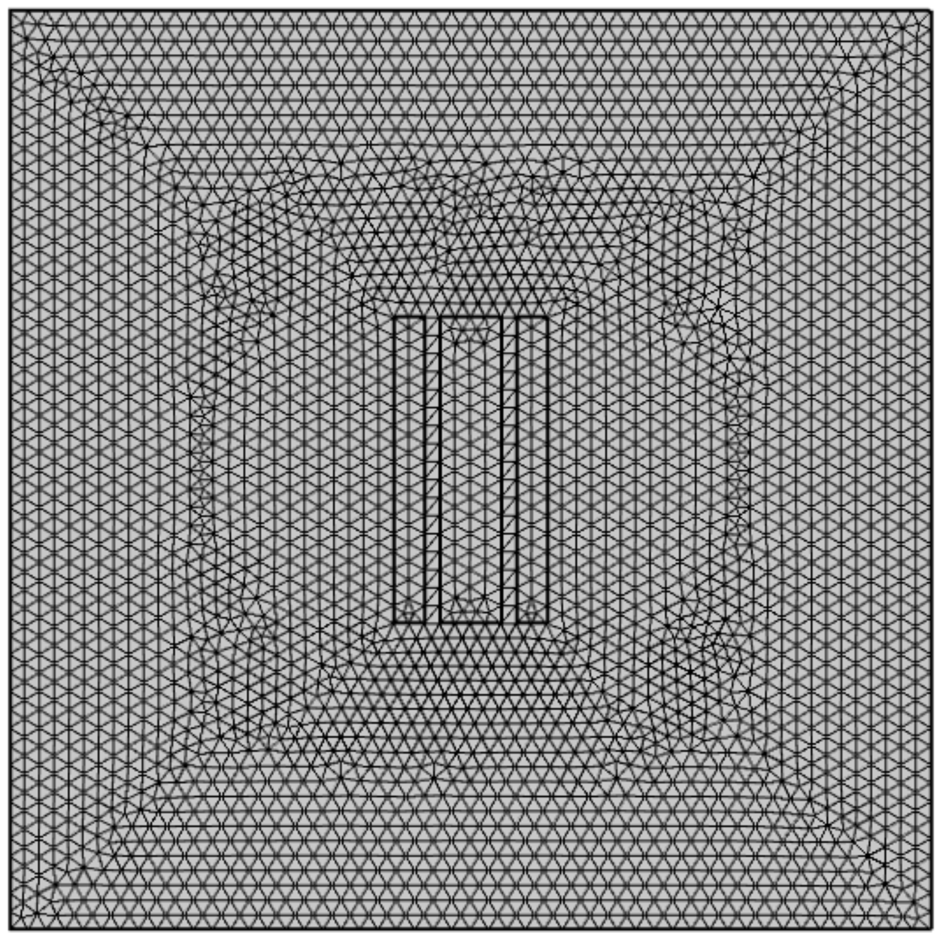
Before solving the physical field, the model needed to be divided into meshes and then used for finite element calculation. Since the magnetic flux density of the magnetic core was mainly calculated and accurate data were required, the meshes were divided into ultra-fine meshes. The grid contained 12,666 cells. The segmentation result is shown in
Figure 6.
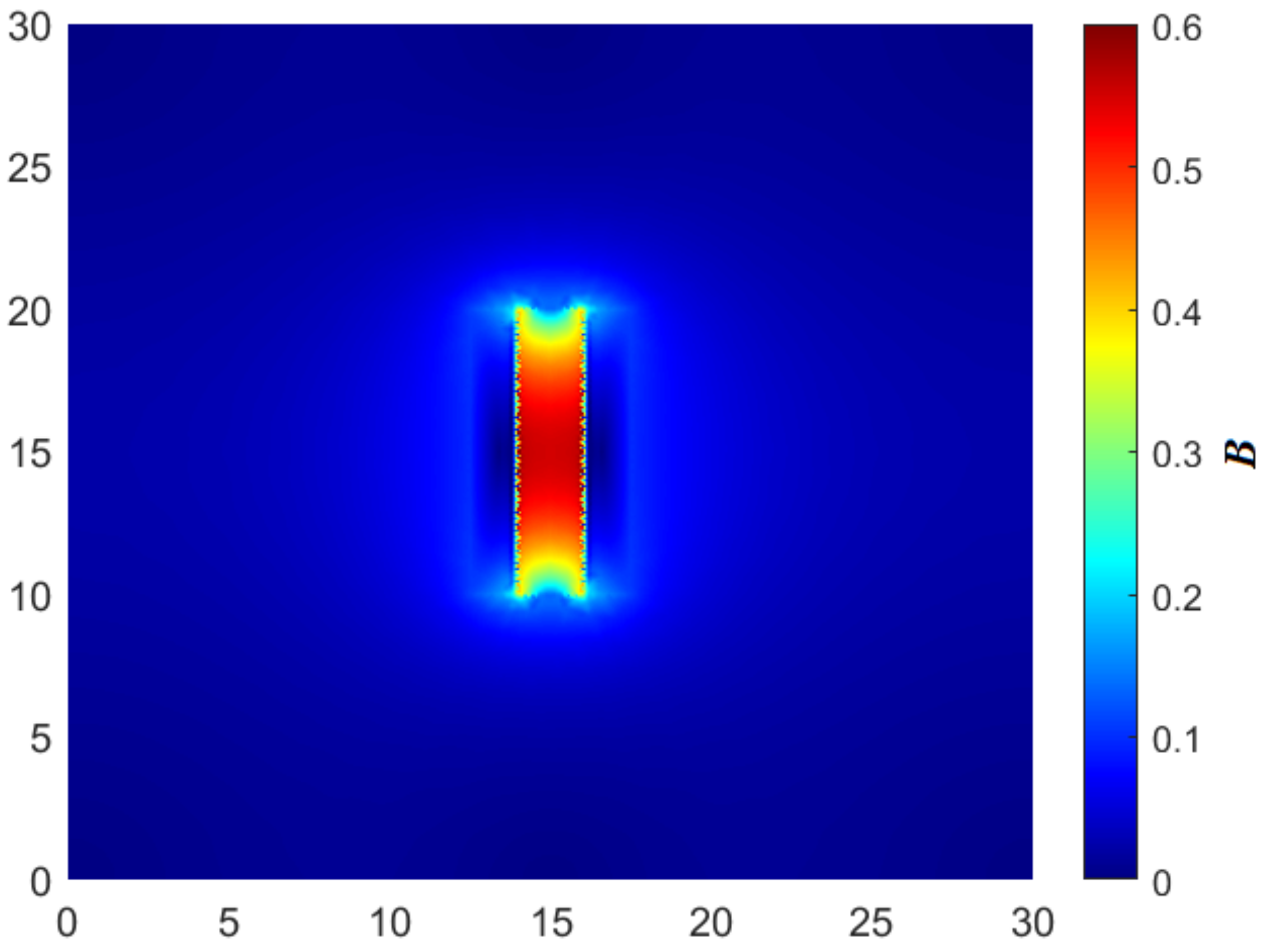
In this paper, the iron core material was silicon steel. When the coil current was 100 A, the relative permeability of the silicon steel was 7000, and the number of winding turns was 100 turns, the finite element calculation result is shown in
Figure 7.
It can be seen from the magnetic flux density cloud diagram that the magnetic flux density in the magnetic core was larger, and the magnetic flux density in the coil was smaller. The magnetic flux density in the air decreased with the distance from the magnetic core.
3.2. Magnetic Field Calculation Based on Neural Network
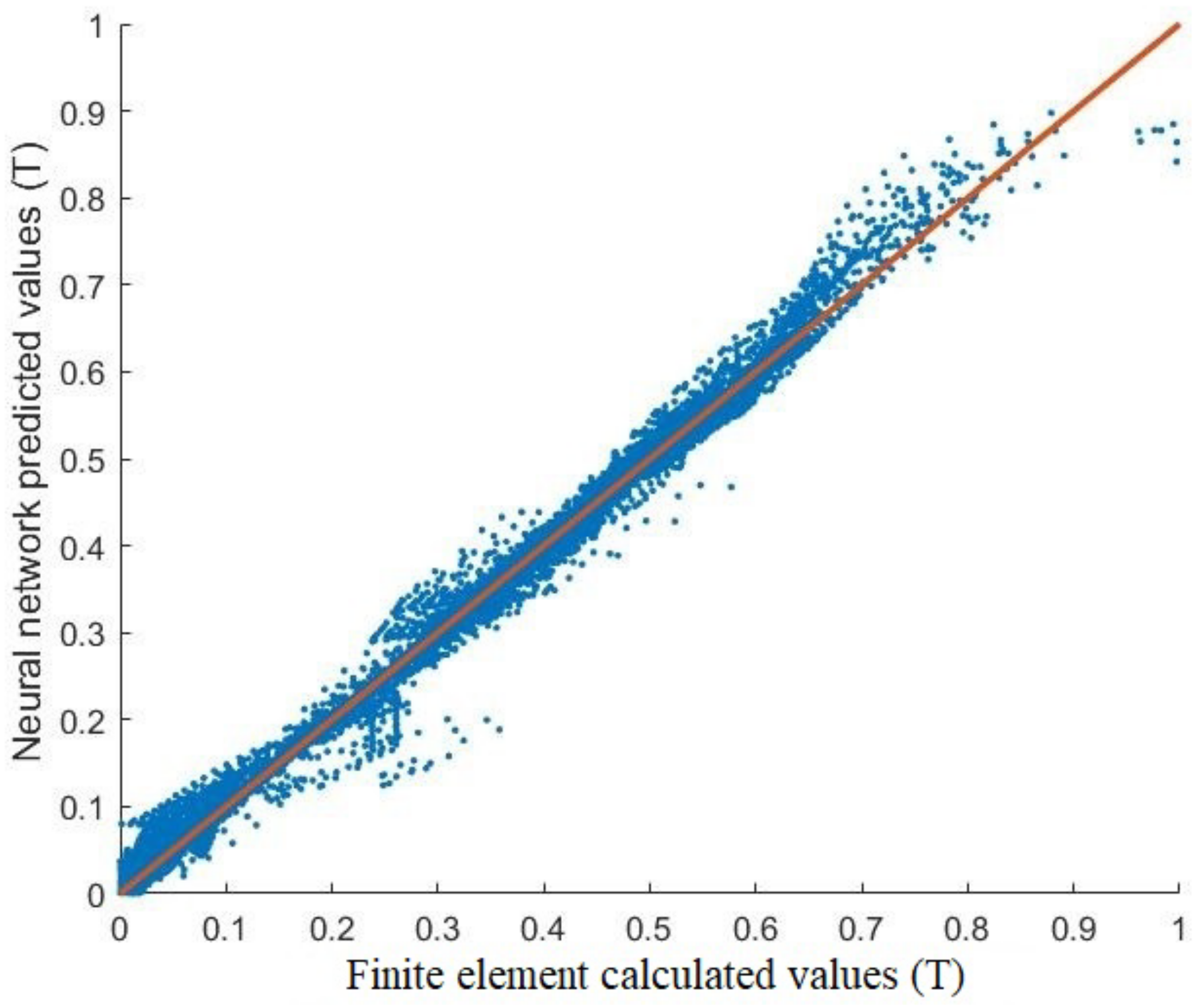
Using finite element calculation, the calculation results were organized into original data. The original data set was divided into a training set and a test set. After the model was generated by learning the data of the training set, the data of the test set was predicted to verify the accuracy of the model. The accuracy R of the neural network method for the learning model of the magnetic field of the inductor with magnetic core was 0.981. It can be seen that the prediction accuracy of the model to the data was relatively high.
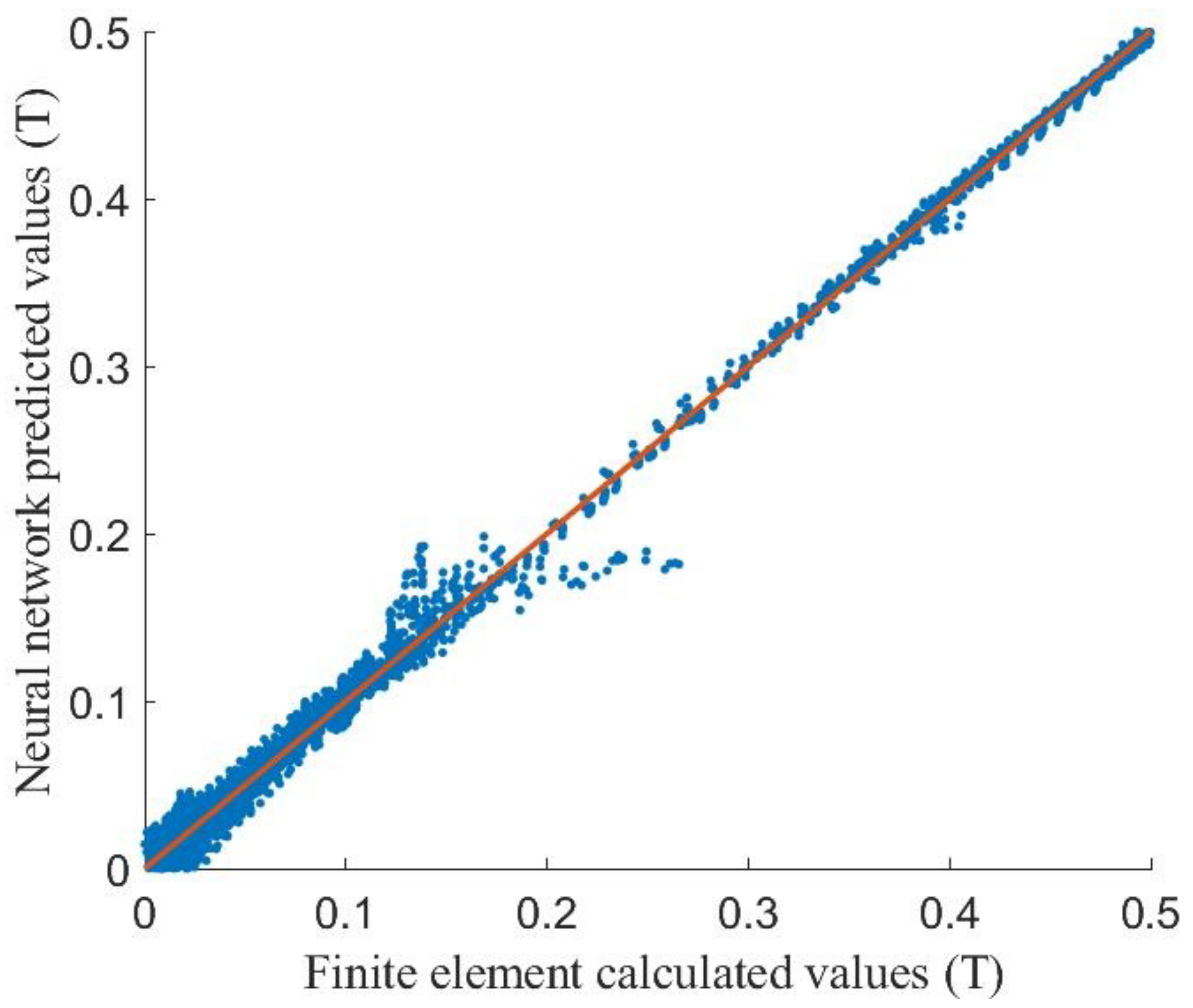
The magnetic flux density predicted by the neural network algorithm was compared with the magnetic flux density calculated by the finite element method, and the results are shown in
Figure 8. Each point in
Figure 8 corresponds to a point in the magnetic field of the cloud image. However, the coordinates of the points in
Figure 8 are not the coordinates in the cloud map; instead, the abscissa is the magnetic flux density calculated by the finite element, and the ordinate is the magnetic flux density predicted by the neural network. The closer the point is to the straight line, the closer the predicted value was to the calculated value, the more accurate the prediction was. It can be seen that the magnetic flux density prediction result by the neural network method was very close to the finite element calculation result, and there was some error between the predicted value and the calculated value near 0.15. In the teaching of the magnetic field of an inductor with a magnetic core, the magnetic field in the magnetic core and its vicinity is worthiest of attention, and the magnetic field in the air domain far away from the magnetic core is secondary. Therefore, as long as the neural network prediction model can guarantee the prediction accuracy within a sufficient range, even if the numerical accuracy of a few points is insufficient, the influence of these points can be ignored, and the final output of the model is valid.
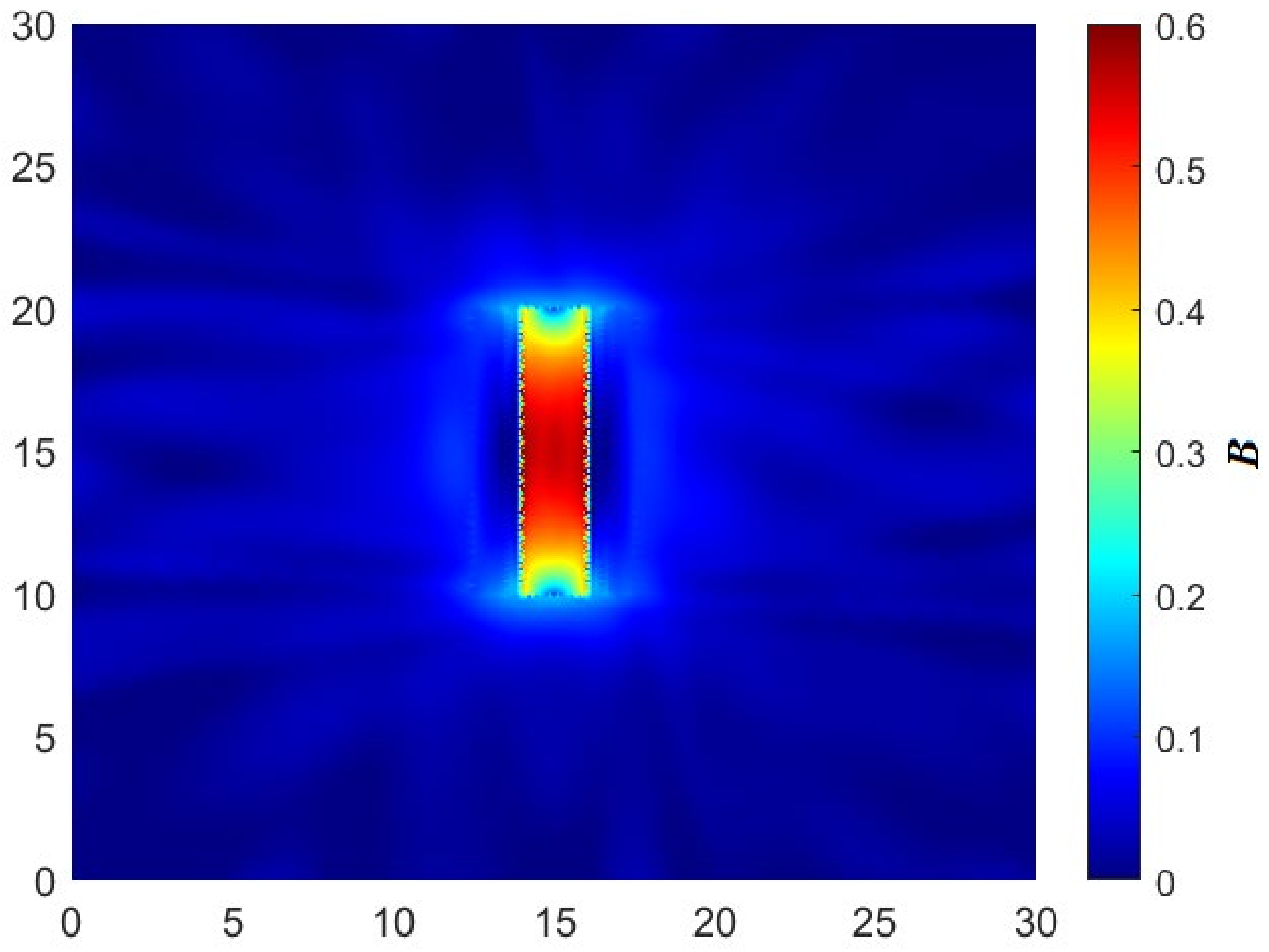
The neural network prediction result of inductor with magnetic core is shown in
Figure 9. It can be seen that the distribution trend of the predicted result in
Figure 9 and the calculated result in
Figure 7 is basically the same. The magnetic flux density in the middle of the magnetic core is the largest, the magnetic flux density at both ends of the magnetic core is smaller, and the magnetic flux density at the tip of the magnetic core is larger. The magnetic flux density in the coil is small, and the magnetic flux density in the air decreases with the increase of the distance from the magnetic core.
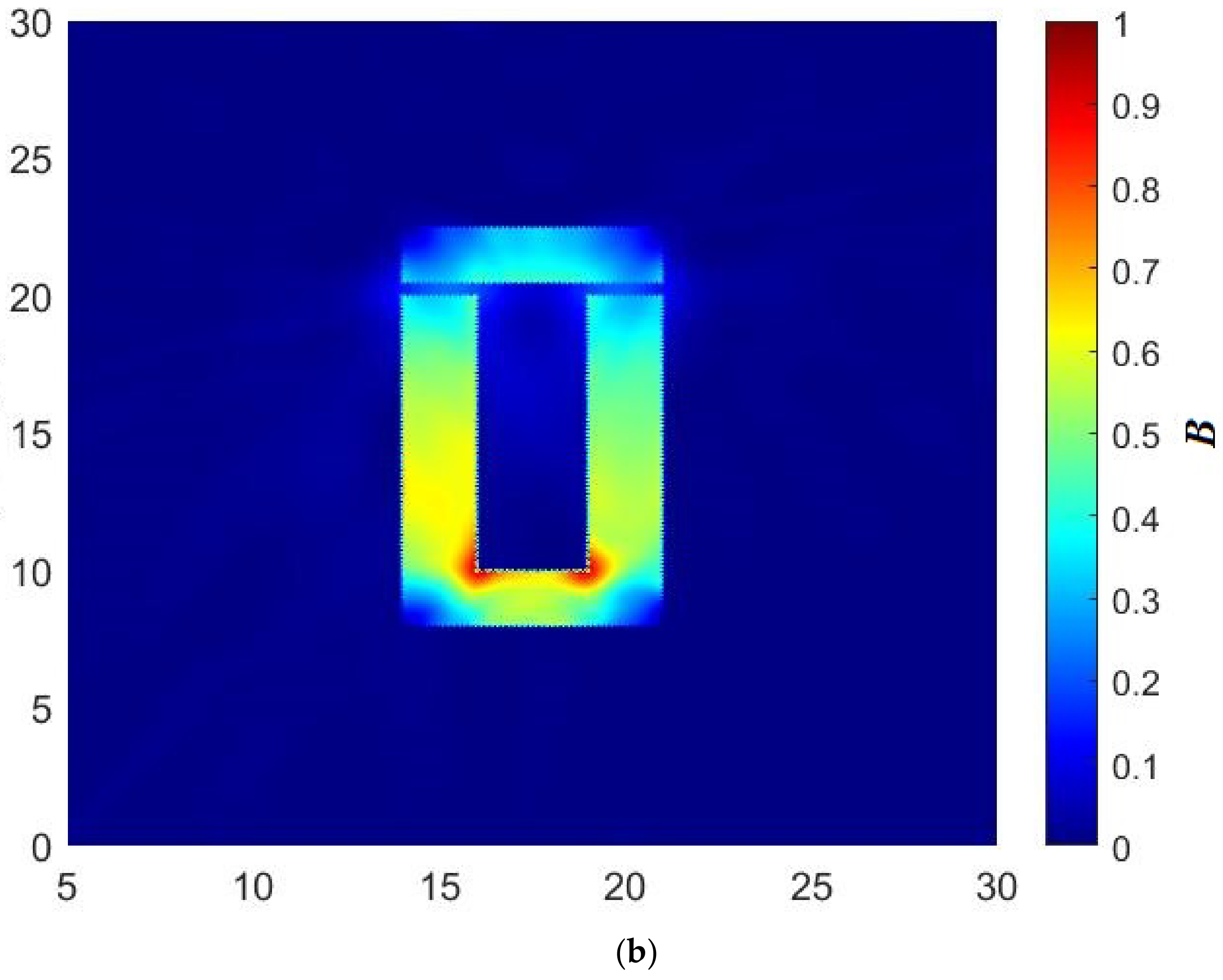
In order to check the accuracy of the neural network model for other shapes of inductor magnetic field calculation, we changed the shape of the inductor and performed the calculation again. The magnetic field cloud diagrams calculated using the finite element and neural network models are shown in
Figure 10.
It can be seen from the figure that the magnetic flux density was concentrated in the iron core, and the magnetic flux density was especially concentrated at the corners of the iron core. The magnetic flux density was smaller near the air gap. The calculation results were more accurate, and the distribution trends of the calculation results and the predicted results were basically the same.
In order to compare the calculation gap between the two more accurately, the different calculated values of each point in the cloud image were compared, as shown in
Figure 11. Each point in the image corresponds to a point in the cloud image. The abscissa is the magnetic flux density calculated by the finite element, and the ordinate is the magnetic flux density predicted by the neural network. The closer the point is to the straight line, the closer the predicted value was to the calculated value, the more accurate the prediction was. It can also be seen that the magnetic flux density prediction result by the neural net-work method was very close to the finite element calculation result, to a degree that can basically meet the needs of magnetic field teaching.
3.3. Magnetic Field Visualization Teaching Platform
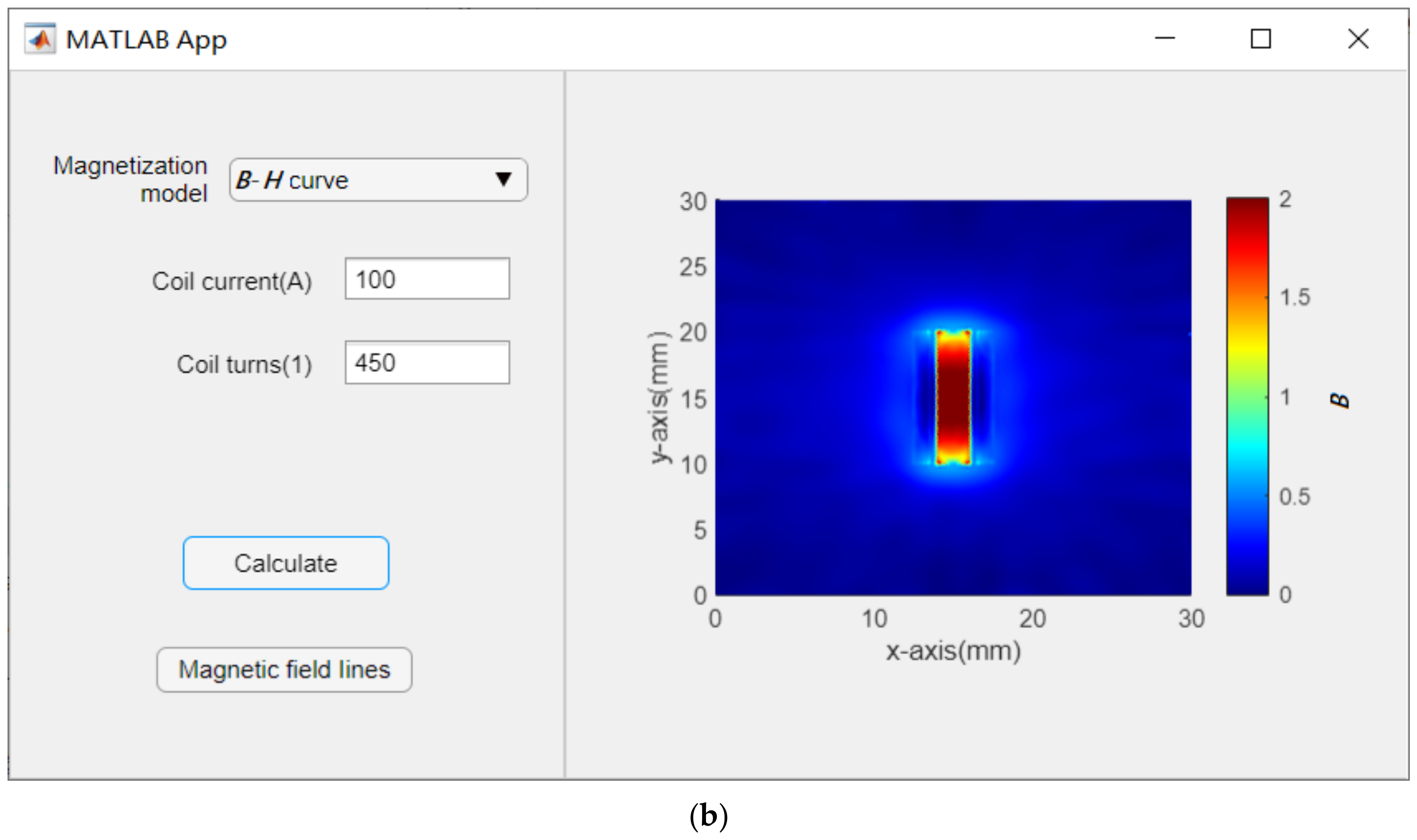
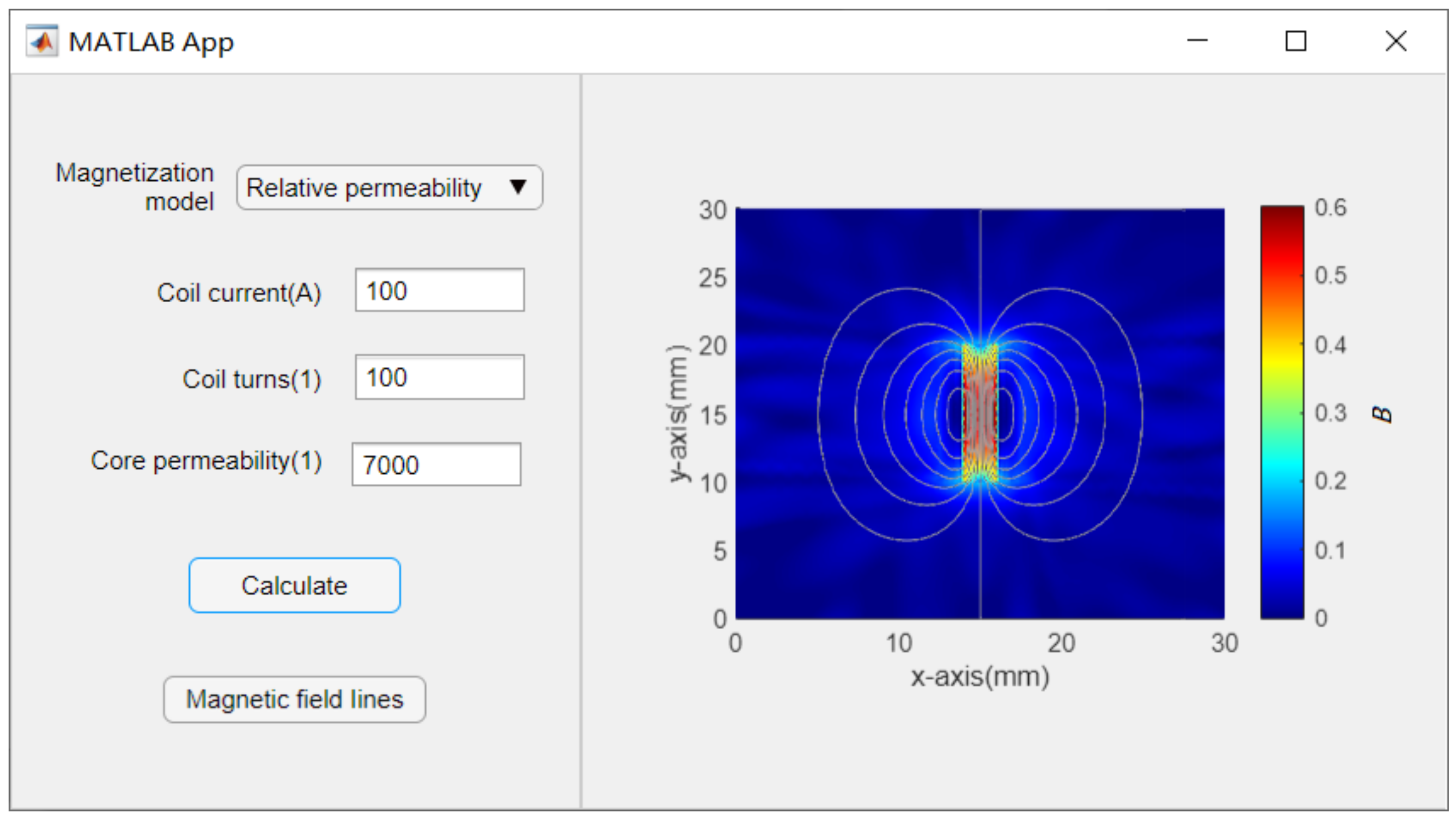
The engineering electromagnetic field visualization teaching software includes two parts: input parameters and calculation drawing. The three parameters of coil current, coil turns, and magnetization model can be changed in the “Input Parameters” menu. The cloud image is calculated after the parameter setting is completed and the “Calculate” button is clicked. After the calculation is completed, the cloud diagram of the calculation result is displayed in the drawing area. Click the “Magnetic field lines” button to display the magnetic field lines. Students can freely set various parameters, obtain the magnetic flux density distribution cloud map of the magnetic core inductor under different parameters through software calculation, and analyze the calculation results. When the core material is linear, students can manually change the relative permeability. When the core material is nonlinear, students can use the
B-
H curve to calculate. When the relative permeability is selected as the magnetization model, an application example is shown in
Figure 12. The version number of MATLAB used is R2016a, from North China Electric Power University, Baoding, China.
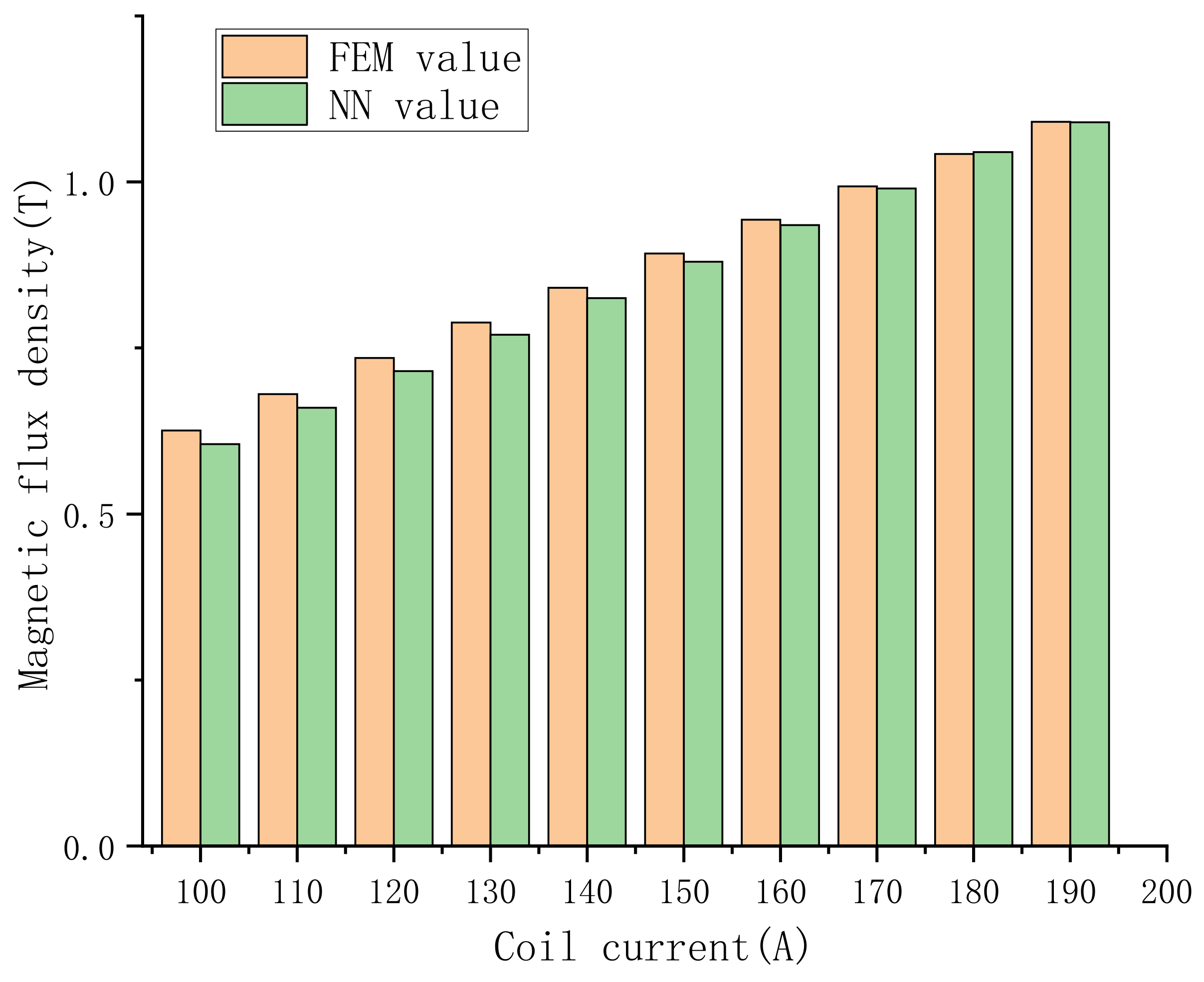
The calculation results obtained by different calculation methods at the same position in the magnetic field were compared statistically. The magnetic flux density at the center point of the inductance was recorded and compared with the finite element calculation value. The results are shown in
Figure 13. It can be seen that the neural network (NN) value was very close to the finite element method (FEM) value for different coil currents. The maximum relative error was about 2.69%, which meets the needs of electromagnetic field teaching and engineering applications.
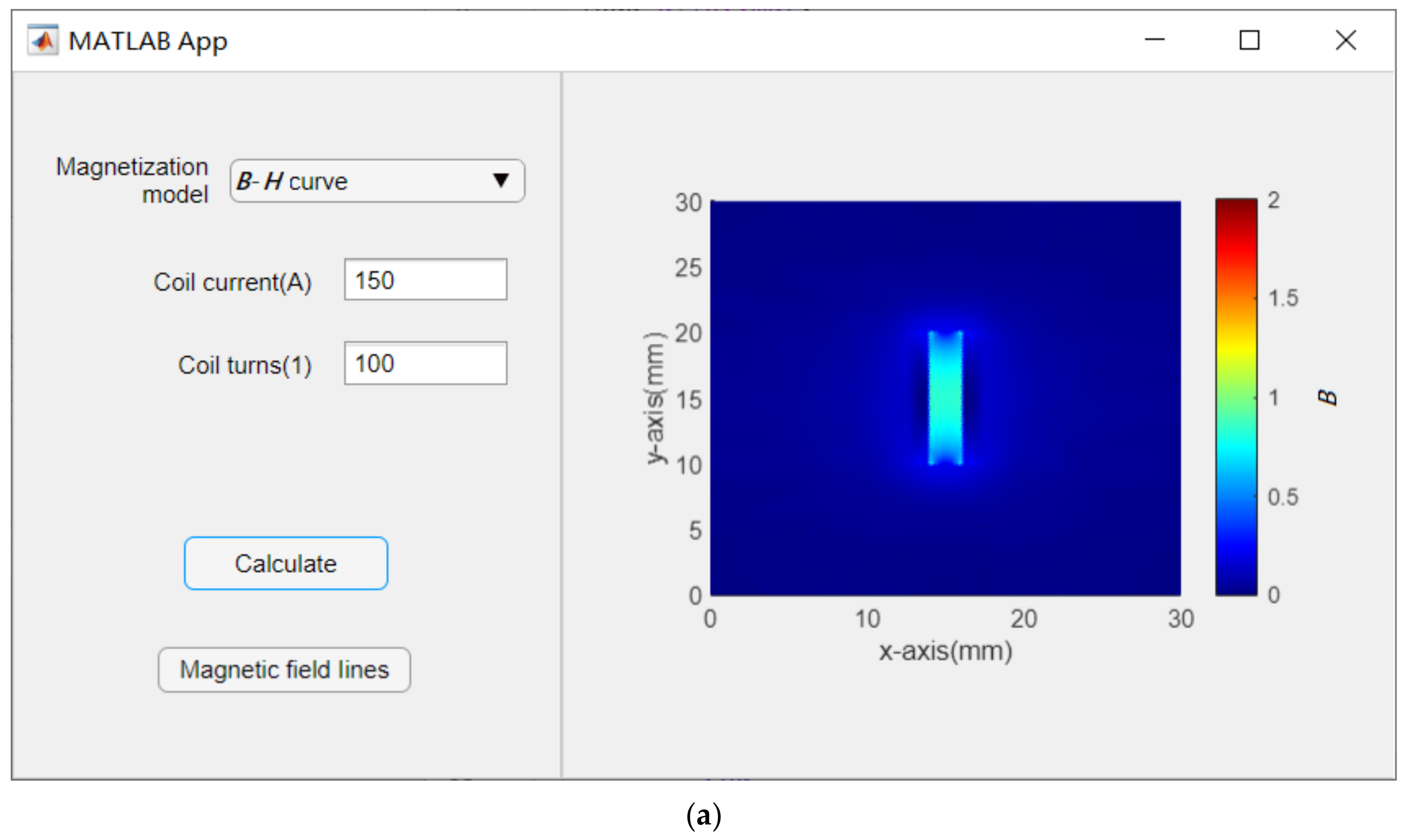
When the magnetization model is the
B-
H curve, the application example is shown in
Figure 14.
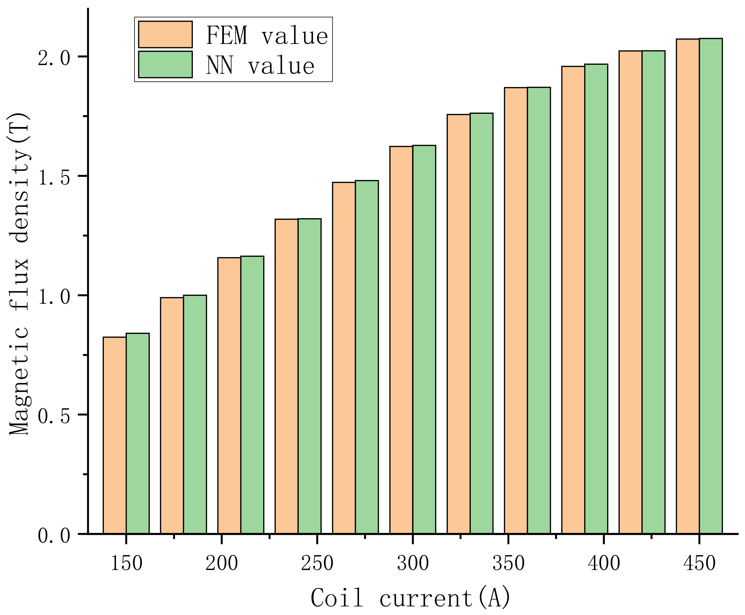
Similar to
Figure 13, the magnetic flux density at the center of the inductor was recorded. The results of comparing the calculated values of the neural network with those calculated by the finite element are shown in
Figure 15. It can be seen that under different working conditions, the maximum relative error of the two calculation methods was about 1.89%. The calculation results meet the needs of electromagnetic field teaching and engineering applications.
The interactive interface of the MATLAB-based magnetic field visualization teaching software is friendly and clear, and the operation steps are simple and easy to learn. In terms of teaching arrangements, teachers can not only demonstrate and lead students to learn about engineering electromagnetic fields in class, but also assign the operation of the visualization software as homework after explaining the relevant theoretical basis, leaving it to the students to explore and complete by themselves. These teaching arrangements can fully mobilize students’ subjective initiative, cultivate students’ autonomous learning ability, and also enable students to consolidate what they have learned after class and deepen their understanding of what they have learned [
25,
26,
27]. Compared with the teaching mode adopted in traditional engineering electromagnetic field classroom teaching, the use of engineering electromagnetic field visualization teaching software to assist teaching has the following advantages:
- (1)
The visualization effect is good. The graphical interface of the engineering electromagnetic field visualization teaching software is easy to control. The software can calculate the electromagnetic field around the inductor with a magnetic core under different material parameters under various working conditions. The calculated results are used to help students intuitively understand the magnetic field characteristics and enhance students’ understanding of theoretical knowledge.
- (2)
The computational efficiency is high. The flow field of the calculation example in the engineering electromagnetic field visualization teaching software is solved by the neural network algorithm. The algorithm has a clear concept, high computational efficiency, and good numerical characteristics. Students can deepen their understanding of the algorithm by combining the implementation process of the neural network algorithm in the software source code.
- (3)
The software lowers the threshold for the use of magnetic field calculation, and is easy to extend to classroom-assisted teaching, reducing teaching costs. Students can learn electromagnetic field theory by directly using the software combined with textbook-related knowledge.
4. Conclusions
In recent years, finite element calculation as well as modern computer graphics and image processing capabilities have advanced by leaps and bounds, while electromagnetic experimental data remain abstract and difficult to understand. Finite element theory and artificial intelligence technology have achieved leapfrog development in the field of electromagnetics. It has become an inevitable trend to carry out electromagnetic experiment teaching through software. In terms of improving the quality of personnel training, strengthening the cultivation of students’ practical and innovative abilities is the fundamental requirement. Experimental teaching is the most common practice method for students in school and is also the most direct way to verify knowledge.
Based on finite element theory and neural network theory, a magnetic field visualization teaching platform was established using finite element calculation and MATLAB software. The experimental platform based on finite element theory is more accurate, but the calculation time is slower; the experimental platform based on neural network theory has a faster calculation time, but the numerical value is slightly wrong. The combination of the two uses the results calculated by the finite element theory as the training data and uses the neural network to establish an experimental platform, so that the results can be calculated more quickly when the experimental requirements are met. Compared with the finite element calculation method, the calculation speed of the magnetic field distribution calculated by the neural network is faster. Taking the calculation of the magnetic core inductance magnetic field as an example, the calculation time can be shortened by about 170 times.
The electromagnetic experiment teaching platform based on a neural network embeds new theoretical knowledge that can not only show students the process of realizing electromagnetic experiments using a deep learning method, but also provide a resource sharing platform and software support services for related scientific research work. The platform can play an important role in improving teaching quality, improving students’ interest in learning as well as their practical ability, and have a positive impact on cultivating comprehensive and innovative talents.
Author Contributions
Conceptualization, G.Y.; methodology, G.Y. and H.L.; validation, G.Y.; writing—original draft preparation, J.L. and D.K.; writing—review and editing, Z.W. and F.L.; project administration, G.Y. All authors have read and agreed to the published version of the manuscript.
Funding
This research was funded by the S&T Program of Hebei (Grant No. 20550901K and No. 21557612K) and University–Industry Collaborative Education Program (Grant No. 201902307005 and No. 202002158011).
Institutional Review Board Statement
Not applicable.
Informed Consent Statement
Not applicable.
Conflicts of Interest
The authors declare no conflict of interest.
References
- Cen, L.; Ruta, D.; Al Qassem, L.M.M.S.; Ng, J. Augmented Immersive Reality (AIR) for Improved Learning Performance: A Quantitative Evaluation. IEEE Trans. Learn. Technol. 2020, 13, 283–296. [Google Scholar] [CrossRef]
- Cmuk, D.; Borsic, M.; Mutapcic, T.; Rapuano, S. A Novel Approach to Remote Teaching: Multilanguage Magnetic Measurement Experiment. IEEE Trans. Instrum. Meas. 2008, 57, 724–730. [Google Scholar] [CrossRef]
- Supriyatno, T.; Kurniawan, F. A New Pedagogy and Online Learning System on Pandemic COVID 19 Era at Islamic Higher Education. In Proceedings of the 2020 6th International Conference on Education and Technology (ICET), Malang, Indonesia, 17 October 2020; pp. 7–10. [Google Scholar]
- Luo, T.; Zhang, M.; Pan, Z.; Li, Z.; Cai, N.; Miao, J.; Chen, Y.; Xu, M. Dream-Experiment: A MR User Interface with Natural Multi-channel Interaction for Virtual Experiments. IEEE Trans. Vis. Comput. Graph. 2020, 26, 3524–3534. [Google Scholar] [CrossRef] [PubMed]
- Fu, S.; Zhao, J.; Cui, W.; Qu, H. Visual Analysis of MOOC Forums with iForum. IEEE Trans. Vis. Comput. Graph. 2017, 23, 201–210. [Google Scholar] [CrossRef]
- Amabili, L.; Gupta, K.; Raidou, R.G. A Taxonomy-Driven Model for Designing Educational Games in Visualization. IEEE Comput. Graph. Appl. 2021, 41, 71–79. [Google Scholar] [CrossRef]
- Massa, A.; Anselmi, N.; Dall’Asta, L.; Gottardi, G.; Goudos, S.K.; Hannan, M.A.; Huang, J.; Li, M.; Oliveri, G.; Poli, L.; et al. Teaching Electromagnetics to Next-Generation Engineers—The ELEDIA Recipe: The ELEDIA teaching style. IEEE Antennas Propag. Mag. 2020, 62, 50–61. [Google Scholar] [CrossRef]
- Notaroš, B.M. Geometrical Approach to Vector Analysis in Electromagnetics Education. IEEE Trans. Educ. 2013, 56, 336–345. [Google Scholar] [CrossRef]
- Warnick, K.F.; Selfridge, R.H.; Arnold, D.V. Teaching electromagnetic field theory using differential forms. IEEE Trans. Educ. 1997, 40, 53–68. [Google Scholar] [CrossRef] [Green Version]
- Stockrahm, A.; Kangas, J.; Kotiuga, P.R. Tools for Visualizing Cuts in Electrical Engineering Education. IEEE Trans. Magn. 2016, 52, 1–4. [Google Scholar] [CrossRef]
- Tan, E.L.; Heh, D.Y. Teaching and Learning Electromagnetic Plane Wave Reflection and Transmission Using 3D TV [Education Corner]. IEEE Antennas Propag. Mag. 2019, 61, 101–108. [Google Scholar] [CrossRef]
- Iskander, M.F. Technology-based electromagnetic education. IEEE Trans. Microw. Theory Tech. 2002, 50, 1015–1020. [Google Scholar] [CrossRef]
- Liao, Z.; Pan, H.; Fan, X.; Zhang, Y.; Kuang, L. Multiple Wavelet Convolutional Neural Network for Short-Term Load Forecasting. IEEE Internet Things J. 2021, 8, 9730–9739. [Google Scholar] [CrossRef]
- Quan, H.; Srinivasan, D.; Khosravi, A. Short-Term Load and Wind Power Forecasting Using Neural Network-Based Prediction Intervals. IEEE Trans. Neural Netw. Learn. Syst. 2014, 25, 303–315. [Google Scholar] [CrossRef]
- Li, L.; Zhang, X.; Wang, Z. Fault Diagnosis in Solar Photovoltaic Grid-Connected Power System Based on Fault Tree and BAM Neural Network. Trans. China Electrotech. Soc. 2015, 30, 248–254. [Google Scholar]
- Xu, C.; Wang, C.; Ying, H.; Yuan, X. FENN Model for 3-D Magnetic Field Calculation. Trans. China Electrotech. Soc. 2012, 27, 125–132. [Google Scholar]
- Adly, A.A.; Abd-El-Hafiz, S.K. Automated two-dimensional field computation in nonlinear magnetic media using Hopfield neural networks. IEEE Trans. Magn. 2002, 38, 2364–2366. [Google Scholar] [CrossRef]
- Adly, A.A.; Abd-El-Hafiz, S.K. Field Computation in Media Exhibiting Hysteresis Using Hopfield Neural Networks. IEEE Trans. Magn. 2022, 58, 1–5. [Google Scholar] [CrossRef]
- Zhu, D. The Research Progress and Prospects of Artificial Neural Networks. J. Cloth. Res. 2004, 1, 101–110. [Google Scholar]
- Mao, J.; Zhao, H.; Yao, Q. Application and prospect of Artificial Neural Network. Electron. Des. Eng. 2011, 19, 62–65. [Google Scholar]
- Jain, A.K.; Duin, R.P.; Mao, J. Statistical pattern recognition: A review. IEEE Trans. Pattern Anal. Mach. Intell. 2000, 22, 4–37. [Google Scholar] [CrossRef] [Green Version]
- Yi, C.; Zhang, Q. Evaluation Model of Sustainable Development for Railway Transportation Based on BP Neural Network. In Proceedings of the 2013 Sixth International Symposium on Computational Intelligence and Design, Hangzhou, China, 28–29 October 2013; pp. 76–79. [Google Scholar]
- Qi, D.; Kang, J. Design of Neural Network. Comput. Eng. Des. 1998, 2, 47–49. [Google Scholar]
- Shen, H.; Wang, Z.; Gao, C.; Qin, J.; Yao, F.; Xu, W. Determining the number of Neural Network Hidden Layer Units. J. Tianjin Univ. Technol. 2008, 5, 13–15. [Google Scholar]
- Trintinalia, L.C. Calculation Tool for the Visualization of EM Wave Reflection and Refraction. IEEE Antennas Propag. Mag. 2013, 55, 203–211. [Google Scholar] [CrossRef]
- D’Aucelli, G.M.; Giaquinto, N.; Andria, G. LineLab-A Transmission Line Simulator for Distributed Sensing Systems: Open-Source MATLAB Code for Simulating Real-World Transmission Lines. IEEE Antennas Propag. Mag. 2018, 60, 22–30. [Google Scholar] [CrossRef]
- Li, P.; Zeng, L.; Shui, A.; Jin, X.; Liu, Y.; Wang, H. Design of Forecast System of Back Propagation Neural Network Based on MATLAB. Comput. Appl. Softw. 2008, 25, 149–150. [Google Scholar]
| Publisher’s Note: MDPI stays neutral with regard to jurisdictional claims in published maps and institutional affiliations. |
© 2022 by the authors. Licensee MDPI, Basel, Switzerland. This article is an open access article distributed under the terms and conditions of the Creative Commons Attribution (CC BY) license (https://creativecommons.org/licenses/by/4.0/).


