
An Urban Traffic Flow Fusion Network Based on a Causal Spatiotemporal Graph Convolution Network


Abstract
:1. Introduction
Related Work
- Non-Depth Learning Method
- Deep Learning Method
2. Preparations
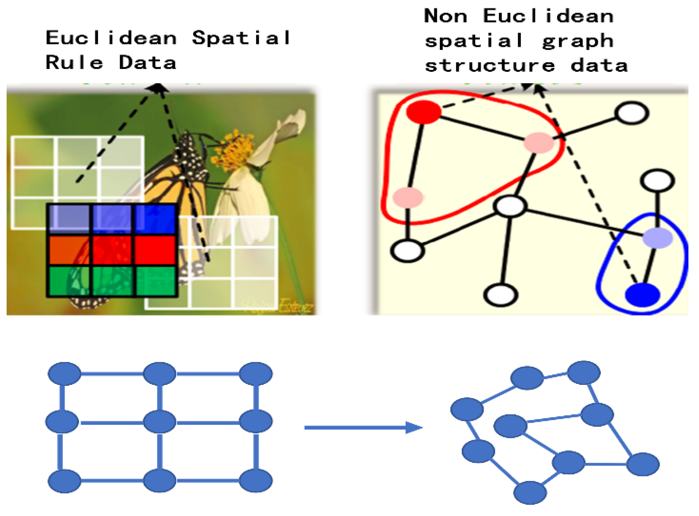
2.1. Traffic Networks
2.2. Graph Neural Networks
3. Model Framework
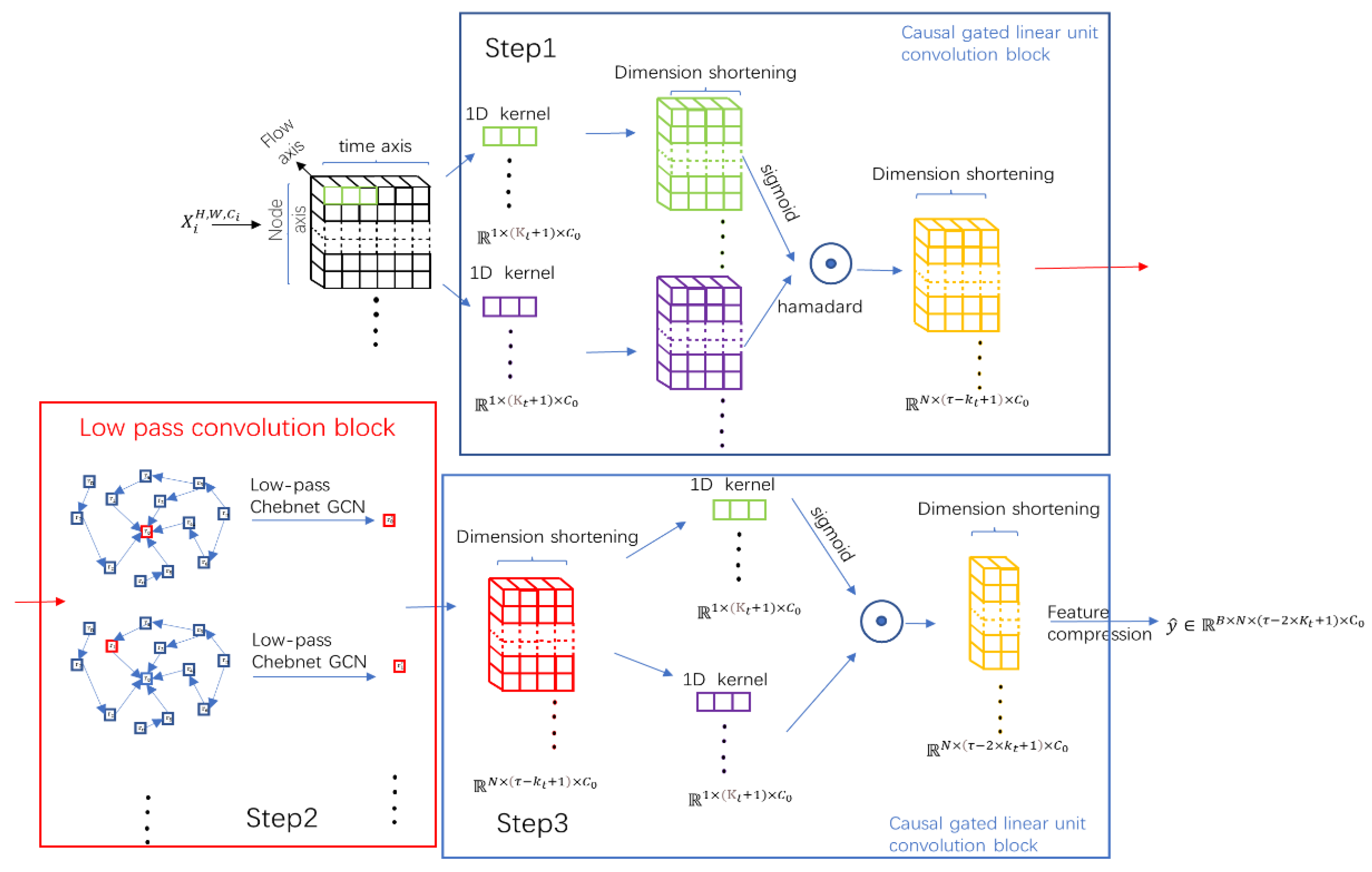
3.1. Network Structure
3.2. LPF Convolution Module
3.3. Causal Gated Linear Unit (C-GLU)
3.4. Fusion of Causal Gated-LPF Convolutions
4. Experiment
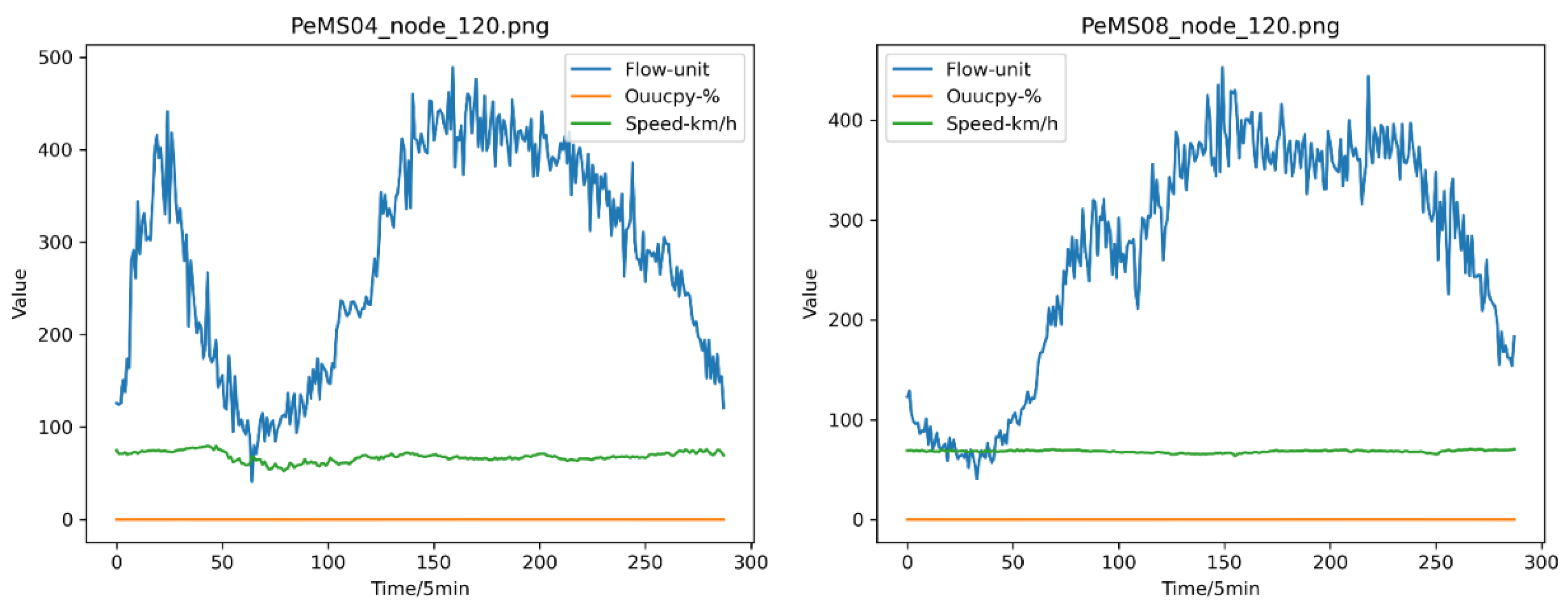
4.1. Data
4.2. Data Processing and Parameter Setting
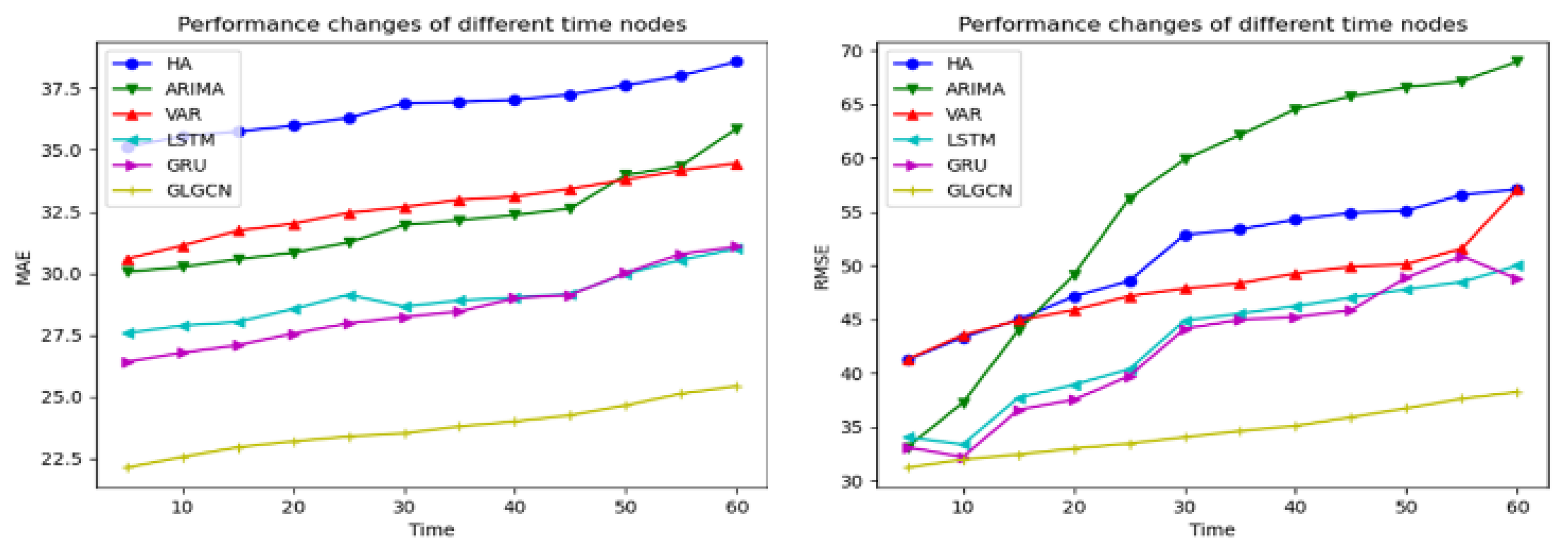
4.3. Analysis and Comparison of Results
5. Conclusions and Outlook
Author Contributions
Funding
Data Availability Statement
Conflicts of Interest
References
- Williams, B.M.; Hoel, L.A. Modeling and forecasting vehicular traffic flow as a seasonal ARIMA process: Theoretical basis and empirical results. J. Transp. Eng. 2003, 129, 664–672. [Google Scholar] [CrossRef] [Green Version]
- Okutani, I.; Stephanedes, Y.J. Dynamic prediction of traffic volume through Kalman filtering theory. Transp. Res. Part B Methodol. 1984, 18, 1–11. [Google Scholar] [CrossRef]
- Kuchipudi, C.M.; Chien, S.I.J. Development of a hybrid model for dynamic travel-time prediction. Transp. Res. Rec. 2003, 1855, 22–31. [Google Scholar] [CrossRef]
- Sun, H.; Liu, H.; Xiao, H.; He, R.R.; Ran, B. Use of Local Linear Regression Model for Short-Term Traffic Forecasting. Transp. Res. Rec. J. Transp. Res. Board 2003, 1836, 143–150. [Google Scholar] [CrossRef]
- Zheng, Y.; Lai, W. High speed short-term traffic flow prediction based on support vector machine. Eng. Constr. 2020, 34, 201–204. [Google Scholar]
- Wu, C.H.; Ho, J.M.; Lee, D.T. Travel-time prediction with support vector regression. IEEE Trans. Intell. Transp. Syst. 2004, 5, 276–281. [Google Scholar] [CrossRef] [Green Version]
- Zhenhua, M.; Kepeng, L.; Dongfu, S. Short-term traffic flow prediction based on wavelet denoising and Bayesian neural network joint model. J. Sci. Technol. Eng. 2020, 20, 13881–13886. [Google Scholar]
- Xu, X.; Bai, Y.; Xu, L. Traffic flow prediction based on Stochastic Forest algorithm in bad weather. J. Shaanxi Norm. Univ. Nat. Sci. Ed. 2020, 48, 25–31. [Google Scholar]
- Ding, C.; Wang, D.; Ma, X.; Li, H. Predicting Short-Term Subway Ridership and Prioritizing Its Influential Factors Using Gradient Boosting Decision Trees. Sustainability 2016, 8, 1100. [Google Scholar] [CrossRef] [Green Version]
- Wang, D.; Zhang, Q.; Wu, S.; Li, X.; Wang, R. Traffic flow forecast with urban transport network. In Proceedings of the 2016 IEEE International Conference on Intelligent Transportation Engineering (ICITE), Singapore, 20–22 August 2016; pp. 139–143. [Google Scholar]
- Park, D.; Rilett, L.R. Forecasting freeway link travel times with a multilayer feedforward neural network. Comput.-Aided Civ. Infrastruct. Eng. 1999, 14, 357–367. [Google Scholar] [CrossRef]
- Dia, H. An object-oriented neural network approach to short-term traffic forecasting. Eur. J. Oper. Res. 2001, 131, 253–261. [Google Scholar] [CrossRef] [Green Version]
- Wu, Y.; Tan, H. Short-term traffic flow forecasting with spatial-temporal correlation in a hybrid deep learning framework. arXiv 2016, arXiv:1612.01022. [Google Scholar]
- Pan, Z.; Liang, Y.; Wang, W.; Yu, Y.; Zheng, Y.; Zhang, J. Urban traffic prediction from spatio-temporal data using deep meta learning. In Proceedings of the 25th ACM SIGKDD International Conference on Knowledge Discovery & Data, Anchorage, AK, USA, 4–8 August 2019; pp. 1720–1730. [Google Scholar]
- Pu, Y.; Wang, W.; Zhu, Q.; Chen, P. Urban short-term traffic flow prediction algorithm based on CNN RESNET LSTM model. J. Beijing Univ. Posts Telecommun. 2020, 43, 9. [Google Scholar]
- Du, S.; Li, T.; Gong, X.; Yang, Y.; Horng, S.J. Traffic flow forecasting based on hybrid deep learning framework. In Proceedings of the 2017 12th International Conference on Intelligent Systems and Knowledge Engineering (ISKE), Nanjing, China, 24–26 November 2017; pp. 1–6. [Google Scholar]
- Yao, H.; Wu, F.; Ke, J.; Tang, X.; Jia, Y.; Lu, S.; Gong, P.; Ye, J.; Li, Z. Deep multi-view spatial-temporal network for taxi demand prediction. In Proceedings of the AAAI Conference on Artificial Intelligence, New Orleans, LA, USA, 2–7 February 2018; p. 32. [Google Scholar]
- Yu, R.; Li, Y.; Shahabi, C.; Demiryurek, U. Deep learning: A generic approach for extreme condition traffic forecasting. In Proceedings of the 2017 SIAM International Conference on Data Mining, Houston, TX, USA, 27–29 April 2017; pp. 777–785. [Google Scholar]
- Shi, X.; Chen, Z.; Wang, H.; Yeung, D.-Y.; Wong, W.K.; Woo, W.C. Convolutional LSTM network: A machine learning approach for precipitation nowcasting. In Proceedings of the Advances in Neural Information Processing Systems, Montreal, QC, Canada, 7–12 December 2015; p. 28. [Google Scholar]
- Yuan, Z.; Zhou, X.; Yang, T. Hetero-convlstm: A deep learning approach to traffic accident prediction on heterogeneous spatio-temporal data. In Proceedings of the 24th ACM SIGKDD International Conference on Knowledge Discovery & Data Mining, London, UK, 19–23 August 2018; pp. 984–992. [Google Scholar]
- Niepert, M.; Ahmed, M.; Kutzkov, K. Learning convolutional neural networks for graphs. In Proceedings of the 33rd International Conference on Machine Learning, New York, NY, USA, 19–24 June 2016; pp. 2014–2023. [Google Scholar]
- Bruna, J.; Zaremba, W.; Szlam, A.; LeCun, Y. Spectral networks and locally connected networks on graphs. arXiv 2013, arXiv:1312.6203. [Google Scholar]
- Seo, Y.; Defferrard, M.; Vandergheynst, P.; Bresson, X. Structured sequence modeling with graph convolutional recurrent networks. In Proceedings of the International Conference on Neural Information Processing, Siem Reap, Cambodia, 13–16 December 2018; Springer: Cham, Switzerland, 2018; pp. 362–373. [Google Scholar]
- Qi, X.; Liao, R.; Jia, J.; Fidler, S.; Urtasun, R. 3d graph neural networks for rgbd semantic segmentation. In Proceedings of the IEEE International Conference on Computer Vision, Venice, Italy, 22–29 October 2017; pp. 5199–5208. [Google Scholar]
- Liu, Y.; Fan, B.; Xiang, S.; Pan, C. Relation-shape convolutional neural network for point cloud analysis. In Proceedings of the IEEE/CVF Conference on Computer Vision and Pattern Recognition, Long Beach, CA, USA, 15–20 June 2019; pp. 8895–8904. [Google Scholar]
- Yin, R.; Li, K.; Zhang, G.; Lu, J. A deeper graph neural network for recommender systems. Knowl.-Based Syst. 2019, 185, 105020. [Google Scholar] [CrossRef]
- Hell, F.; Taha, Y.; Hinz, G.; Heibei, S.; Müller, H.; Knoll, A. Graph Convolutional Neural Network for a Pharmacy Cross-Selling Recommender System. Information 2020, 11, 525. [Google Scholar] [CrossRef]
- Li, Y.; Yu, R.; Shahabi, C.; Liu, Y. Diffusion convolutional recurrent neural network: Data-driven traffic forecasting. arXiv 2017, arXiv:1707.01926. [Google Scholar]
- Yu, B.; Yin, H.; Zhu, Z. Spatio-temporal graph convolutional networks: A deep learning framework for traffic forecasting. arXiv 2018, arXiv:1709.04875. [Google Scholar]
- Guo, S.; Lin, Y.; Feng, N.; Song, C.; Wan, H. Attention based spatial-temporal graph convolutional networks for traffic flow forecasting. In Proceedings of the Thirty-Third AAAI Conference on Artificial Intelligence, Honolulu, HI, USA, 27 January–1 February 2019; Volume 33, pp. 922–929. [Google Scholar]
- Geng, X.; Li, Y.; Wang, L.; Yang, Q.; Ye, J.; Liu, Y. Spatiotemporal multi-graph convolution network for ride-hailing demand forecasting. In Proceedings of the AAAI Conference on Artificial Intelligence, Honolulu, HI, USA, 27 January–1 February 2019; Volume 33, pp. 3656–3663. [Google Scholar]
- Zhong, W.; Suo, Q.; Jia, X.; Zhang, A.; Su, L. Heterogeneous Spatio-Temporal Graph Convolution Network for Traffic Forecasting with Missing Values. In Proceedings of the 2021 IEEE 41st International Conference on Distributed Computing Systems (ICDCS), Washington, DC, USA, 7–10 July 2021; pp. 707–717. [Google Scholar]
- Siddiqi, M.D.; Jiang, B.; Asadi, R.; Regan, A. Hyperparameter Tuning to Optimize Implementations of Denoising Autoencoders for Imputation of Missing Spatio-temporal Data. Procedia Comput. Sci. 2021, 184, 107–114. [Google Scholar] [CrossRef]
- Joelianto, E.; Fathurrahman, M.F.; Sutarto, H.Y.; Semanjski, I.; Putri, A.; Gautama, S. Analysis of Spatiotemporal Data Imputation Methods for Traffic Flow Data in Urban Networks. ISPRS Int. J. Geo-Inf. 2022, 11, 310. [Google Scholar] [CrossRef]
- Liu, D.; Xu, X.; Xu, W.; Zhu, B. Graph Convolutional Network: Traffic Speed Prediction Fused with Traffic Flow Data. Sensors 2021, 21, 6402. [Google Scholar] [CrossRef] [PubMed]
- Henaff, M.; Bruna, J.; LeCun, Y. Deep convolutional networks on graph-structured data. arXiv 2015, arXiv:1506.05163. [Google Scholar]
- Gehring, J.; Auli, M.; Grangier, D.; Yarats, D.; Dauphin, Y.N. Convolutional sequence to sequence learning. In Proceedings of the International Conference on Machine Learning, Ningbo, China, 9–12 July 2017; pp. 1243–1252. [Google Scholar]


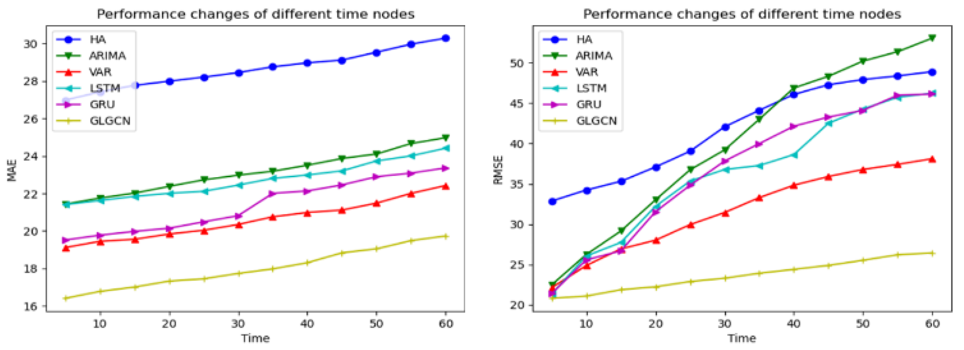
| Model | PeMS04 (5/15/30/45 min) | Model | PeMS08 (5/15/30/45 min) | ||
|---|---|---|---|---|---|
| MAE | RMSE | MAE | RMSE | ||
| HA | 35.12/35.75/36.89/37.25 | 41.25/44.97/52.87/54.89 | HA | 26.98/27.77/28.45/29.12 | 32.87/35.31/42.08/47.29 |
| ARIMA | 30.06/30.56/31.95/32.63 | 33.12/43.98/59.87/65.73 | ARIMA | 21.43/22.02/22.98/23.87 | 22.47/29.15/39.21/48.34 |
| VAR | 30.58/31.72/32.69/33.52 | 46.29/49.92/52.87/54.89 | VAR | 19.19/19.56/20.35/21.12 | 22.12/26.93/31.45/35.91 |
| LSTM | 27.57/28.03/28.65/29.15 | 34.05/37.72/44.89/47.01 | LSTM | 21.41/21.85/22.45/23.21 | 21.32/27.73/36.78/42.51 |
| GRU | 26.41/27.08/28.23/29.12 | 34.12/37.59/45.12/46.85 | GRU | 19.52/19.98/20.82/22.46 | 21.39/26.69/37.83/43.28 |
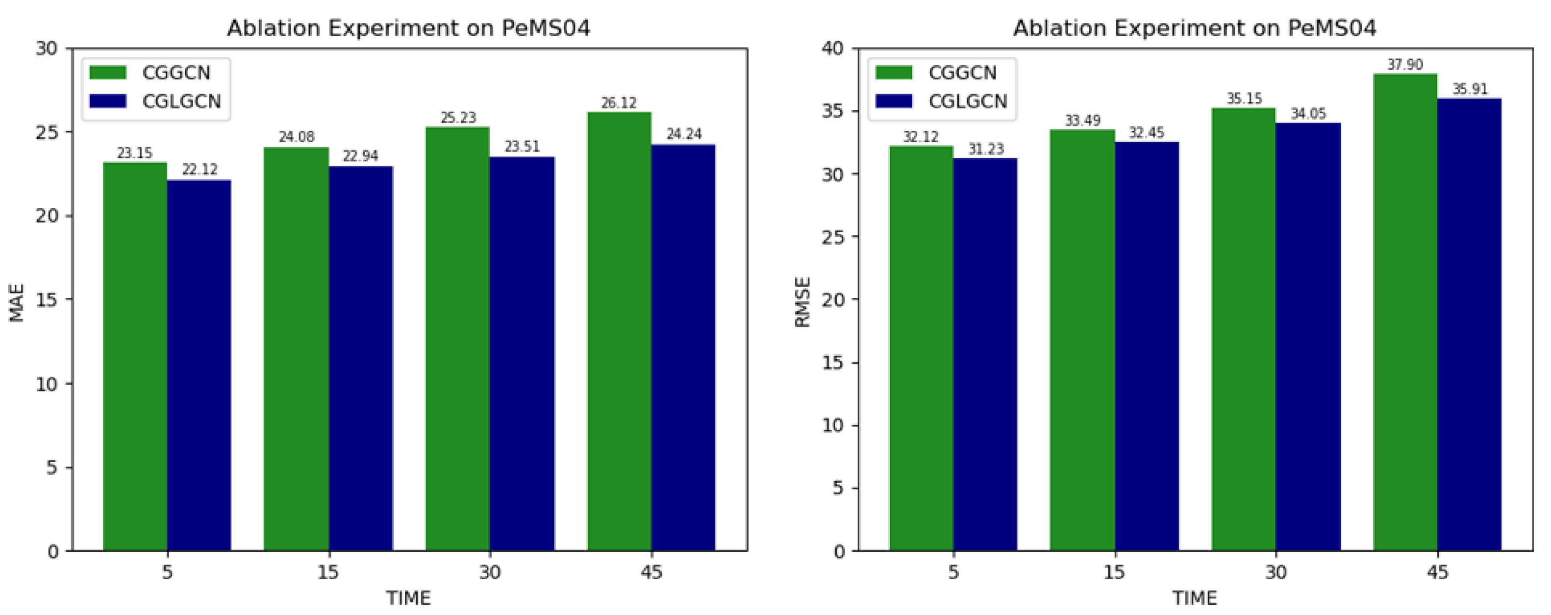
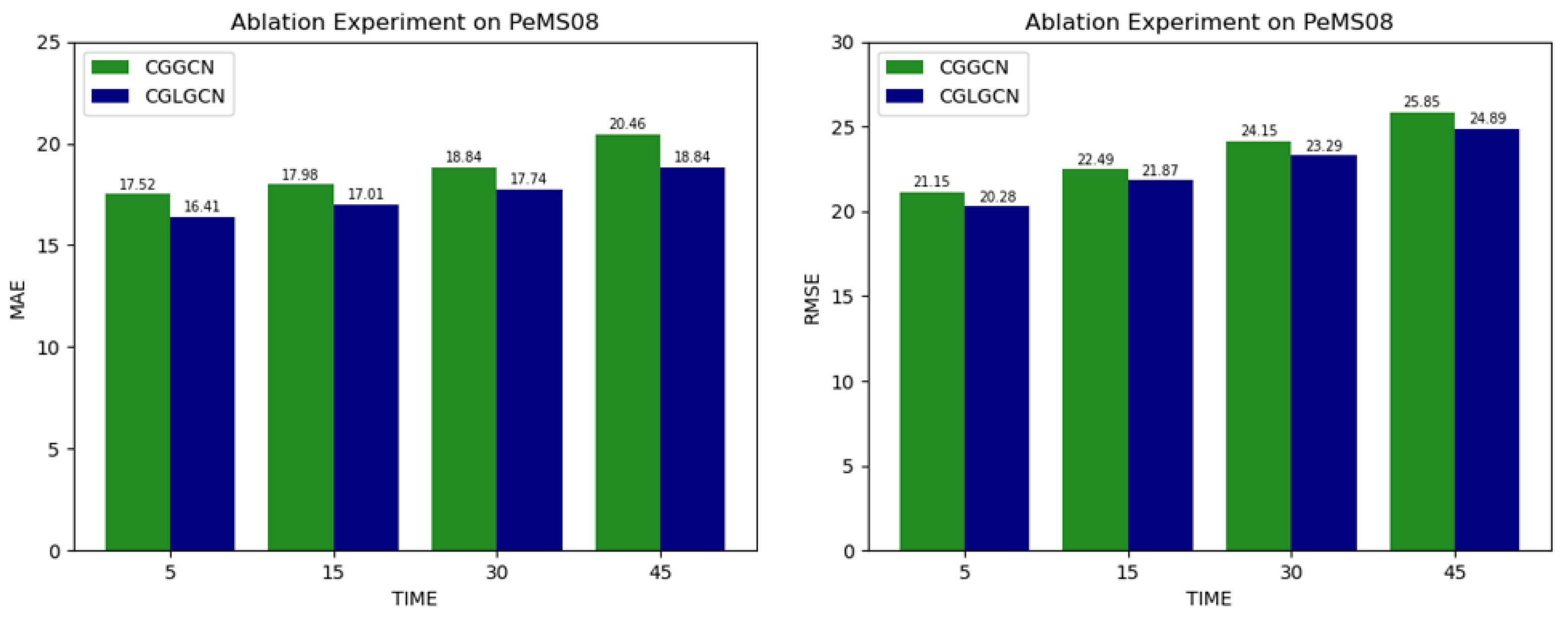
| CGGCN | 23.15/24.08/25.23/26.12 | 32.12/33.49/35.15/37.90 | CGGCN | 17.52/17.98/18.84/20.46 | 21.15/22.49/24.15/25.85 |
| CGLGCN | 22.12/22.94/23.51/24.24 | 31.23/32.45/34.05/35.91 | CGLGCN | 16.41/170.1/17.74/18.84 | 20.28/21.87/23.29/24.89 |
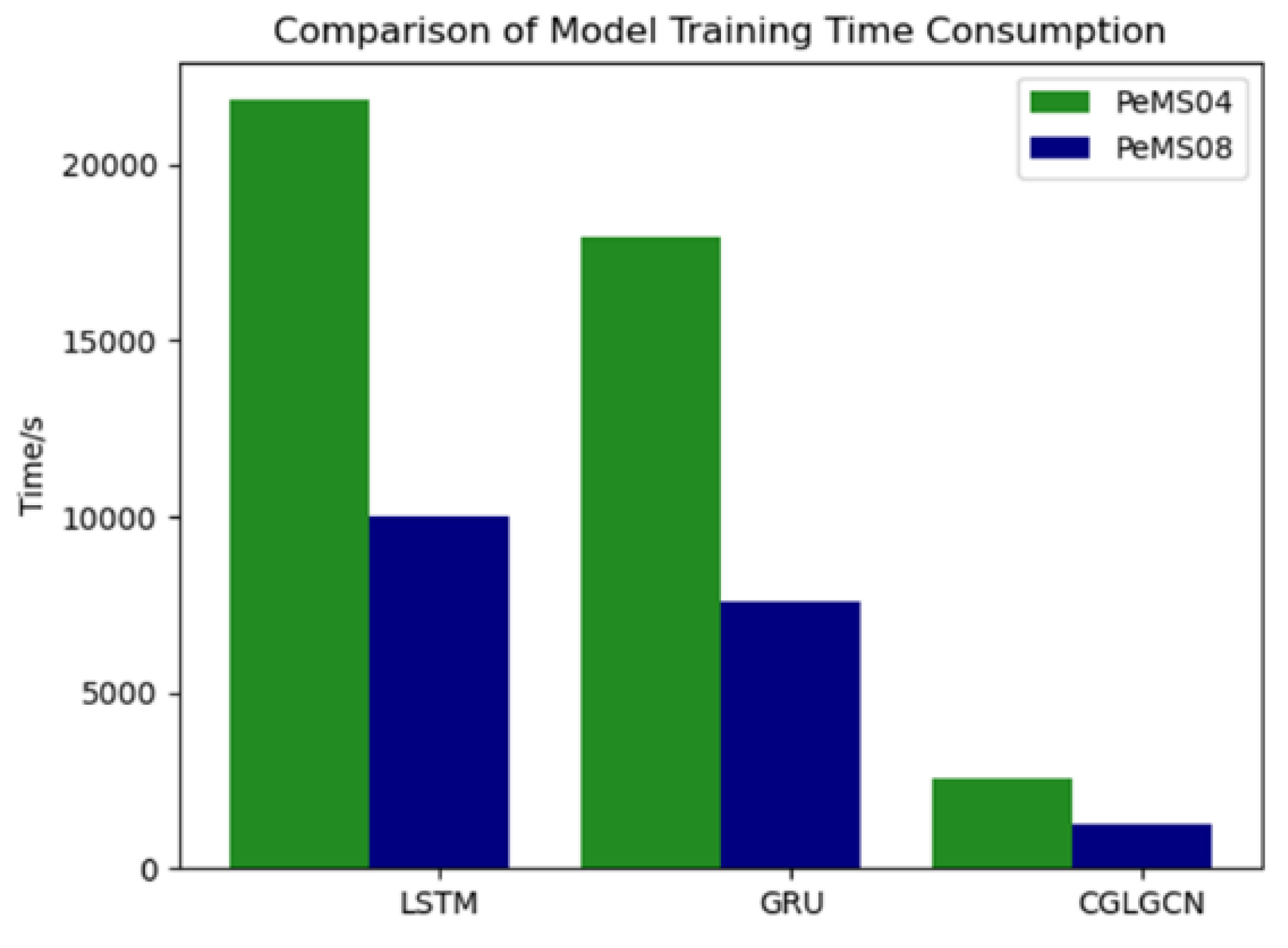
| Dataset | 1000 Epoch Time Consumption (s) | ||
|---|---|---|---|
| LSTM | GRU | CGLGCN | |
| PeMS04 | 21,844.54 | 17,973.62 | 2579.79 |
| PeMS08 | 10,000.15 | 7589.26 | 1279.83 |
Publisher’s Note: MDPI stays neutral with regard to jurisdictional claims in published maps and institutional affiliations. |
© 2022 by the authors. Licensee MDPI, Basel, Switzerland. This article is an open access article distributed under the terms and conditions of the Creative Commons Attribution (CC BY) license (https://creativecommons.org/licenses/by/4.0/).
Share and Cite
Xu, X.; Mao, H.; Zhao, Y.; Lü, X. An Urban Traffic Flow Fusion Network Based on a Causal Spatiotemporal Graph Convolution Network. Appl. Sci. 2022, 12, 7010. https://doi.org/10.3390/app12147010
Xu X, Mao H, Zhao Y, Lü X. An Urban Traffic Flow Fusion Network Based on a Causal Spatiotemporal Graph Convolution Network. Applied Sciences. 2022; 12(14):7010. https://doi.org/10.3390/app12147010
Chicago/Turabian StyleXu, Xing, Hao Mao, Yun Zhao, and Xiaoshu Lü. 2022. "An Urban Traffic Flow Fusion Network Based on a Causal Spatiotemporal Graph Convolution Network" Applied Sciences 12, no. 14: 7010. https://doi.org/10.3390/app12147010
APA StyleXu, X., Mao, H., Zhao, Y., & Lü, X. (2022). An Urban Traffic Flow Fusion Network Based on a Causal Spatiotemporal Graph Convolution Network. Applied Sciences, 12(14), 7010. https://doi.org/10.3390/app12147010