
Channel-Wise Average Pooling and 1D Pixel-Shuffle Denoising Autoencoder for Electrode Motion Artifact Removal in ECG


Abstract
:1. Introduction
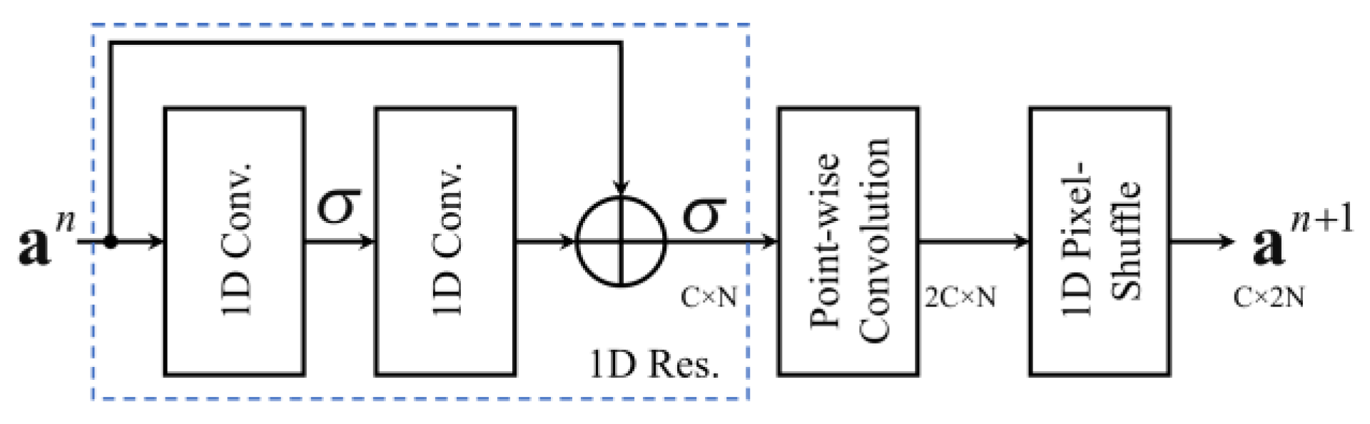
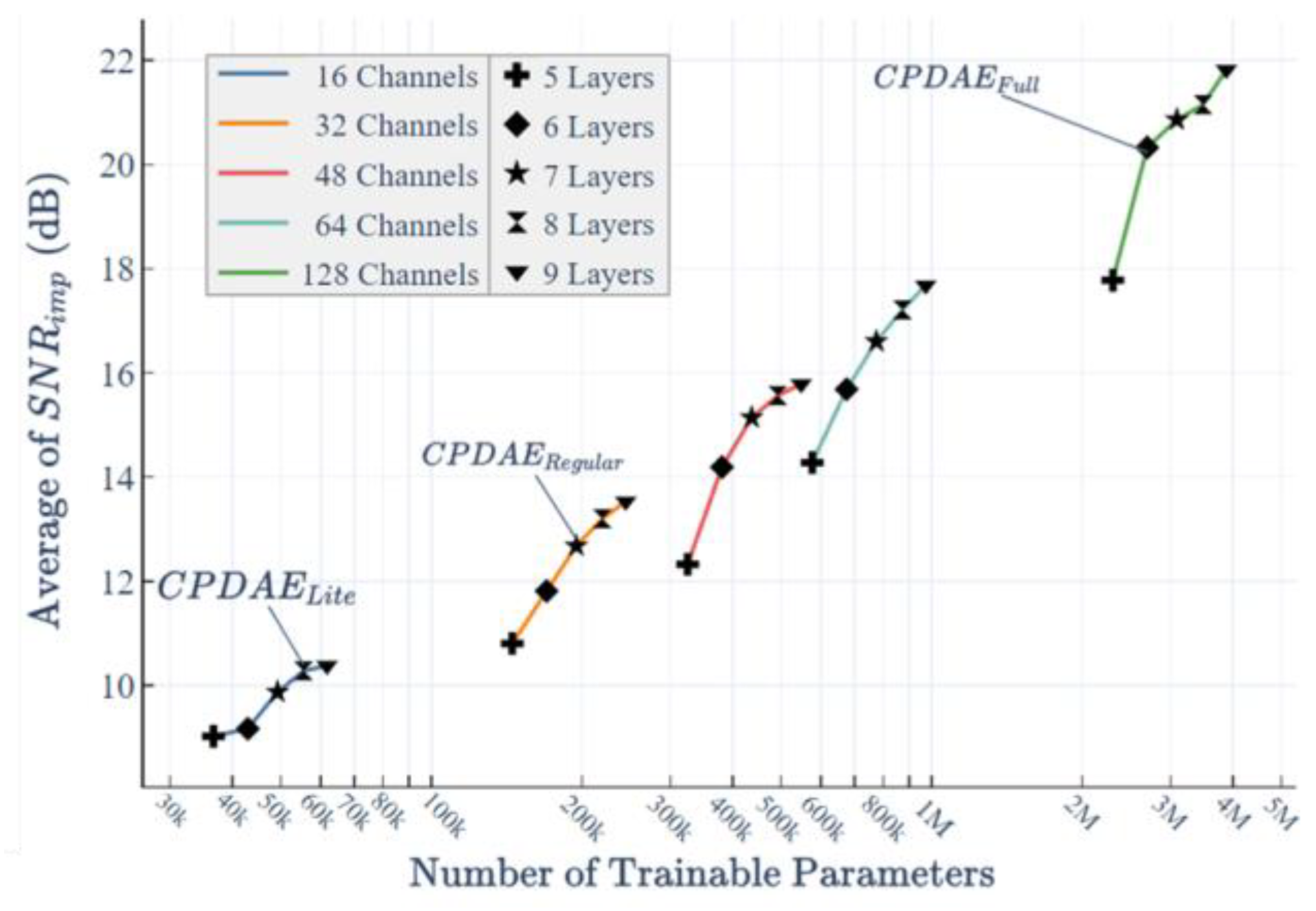
- The schemes of the residual block, pixel shuffle, and CWAP layer are utilized in the proposed DAE for enhancing the feature extracting capability, and the results show that the proposed CPDAE, which uses fewer parameters, can achieve better denoising performance than state-of-the-art approaches.
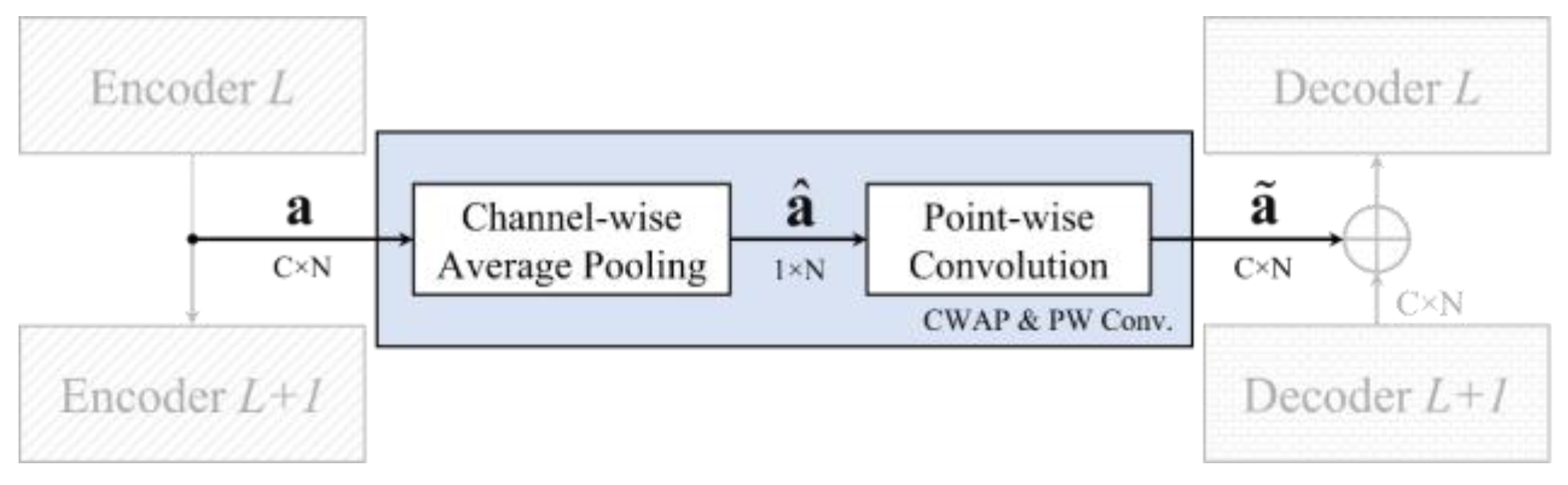
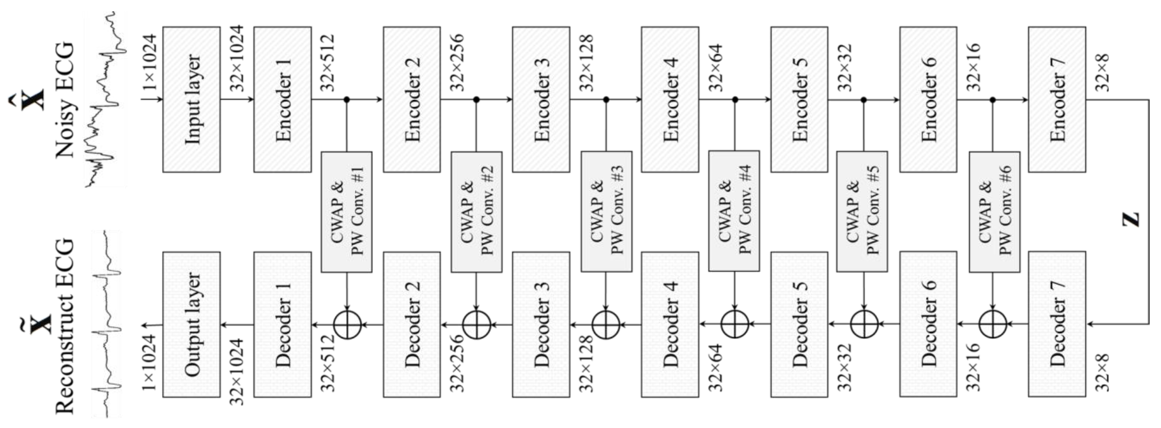
- The proposed CWAP layer between encoder and decoder not only avoids the ECG features disappearing through the deeper encoder layer, but also uses less memory than the shortcut connection. Furthermore, the key features are all averaged in the
- CWAP layer so that the number of channels is greatly reduced to one channel, and this also implies that it only takes 1/C times the memory size in implementation.
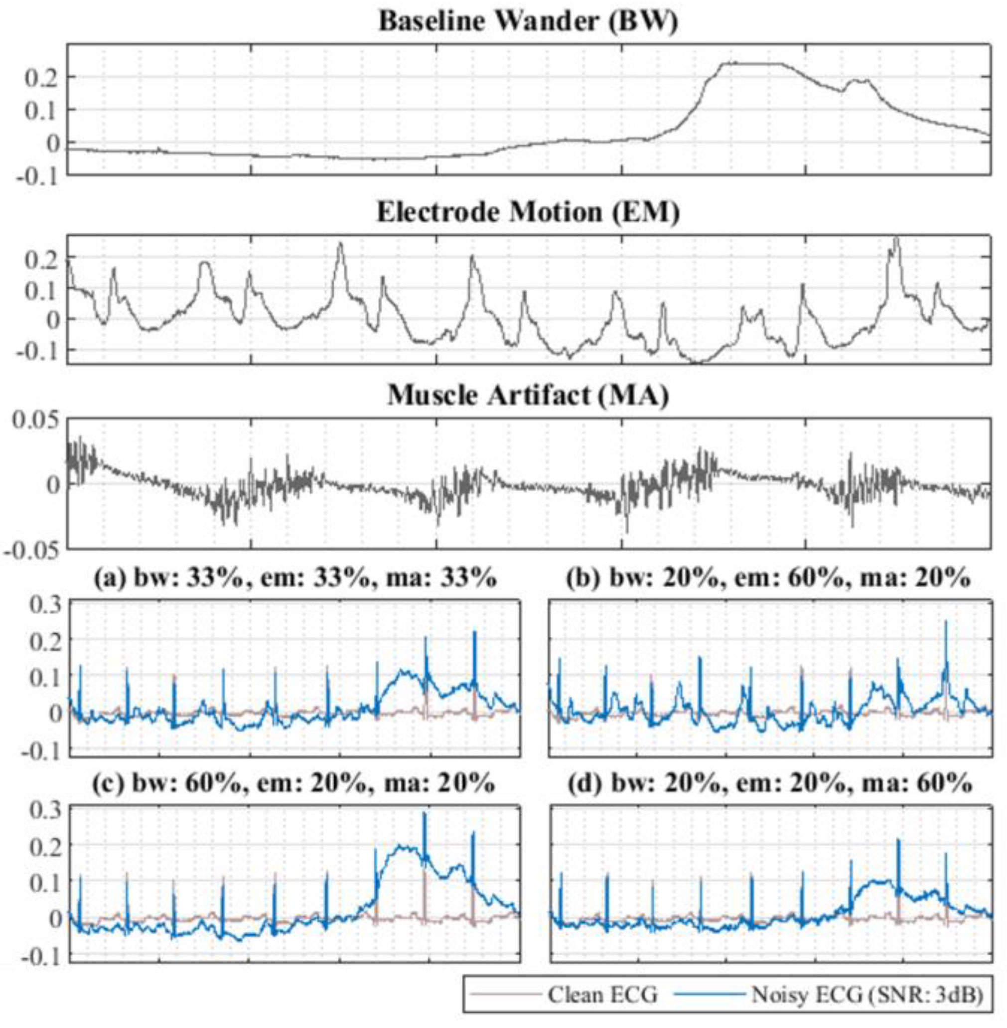
- The noisy ECG dataset obtained from NSTDB dataset is adopted to evaluate the denoising performance for various algorithms under the same conditions to ensure the same experimental environment can be completely rebuilt.
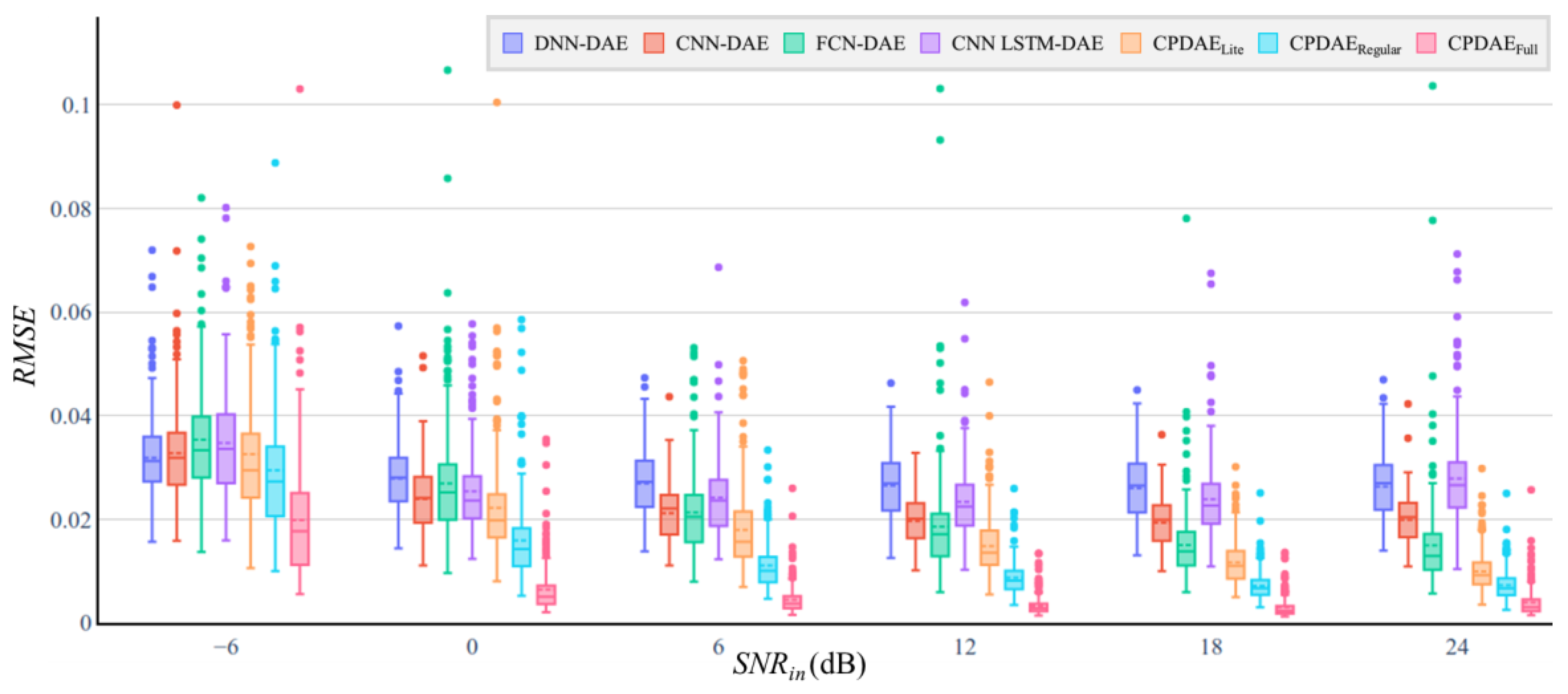
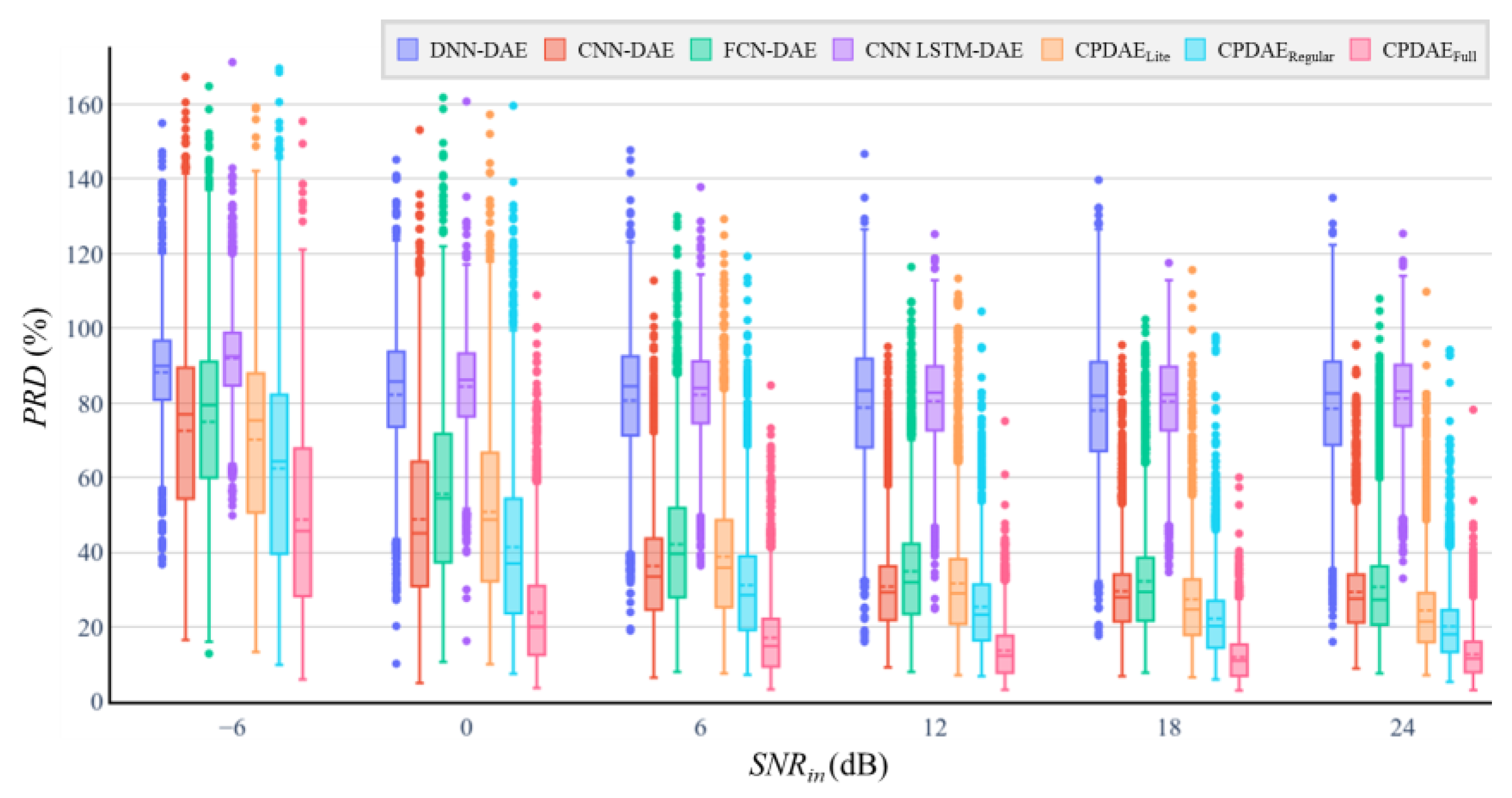
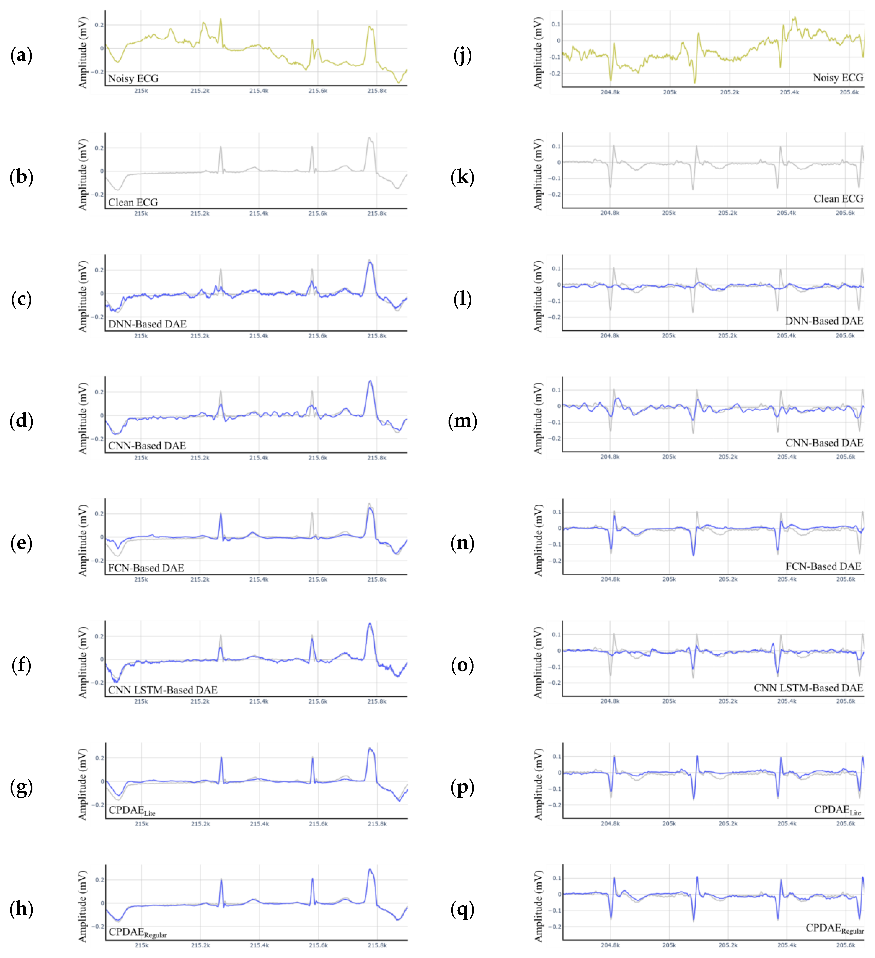
- To test the generalizability of various DAE models, the other noisy ECG dataset with six noise-level inputs is generated by randomly mixing the first 30 min section of the ECG signal in NSRDB with the 30 min section of EM noise in NSTDB. The experimental results demonstrate that the proposed CPDAE has better noise suppression than other approaches.
2. Methodology
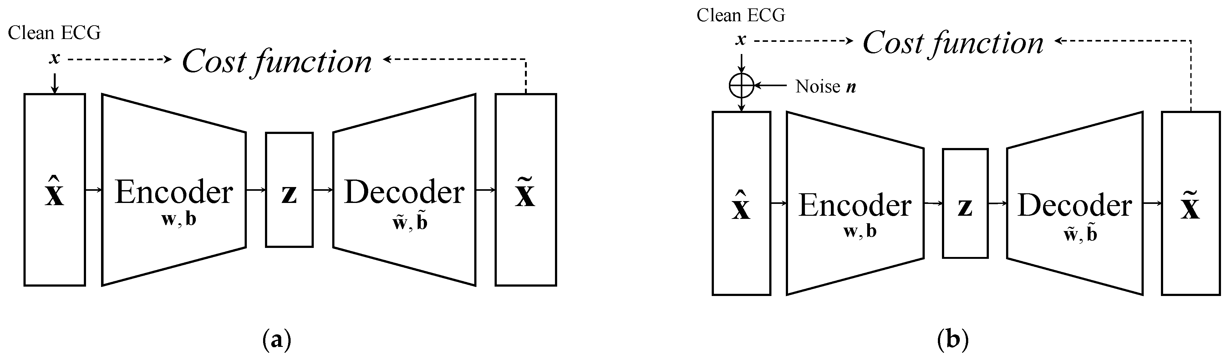
2.1. Review of AE and DAE
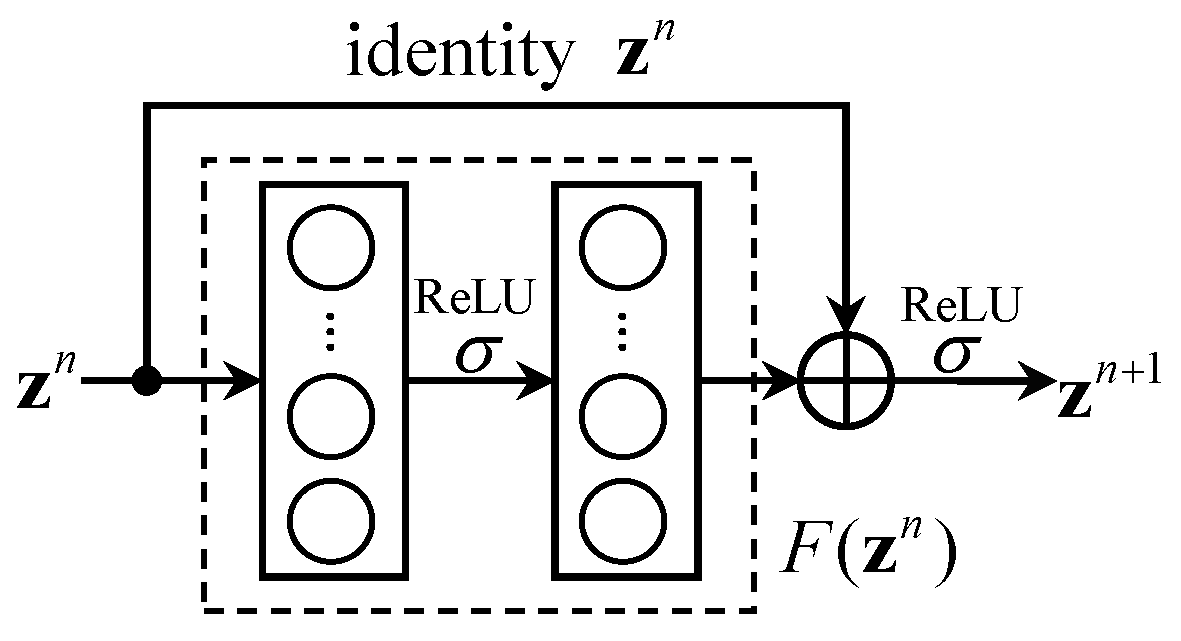
2.2. Residual Block
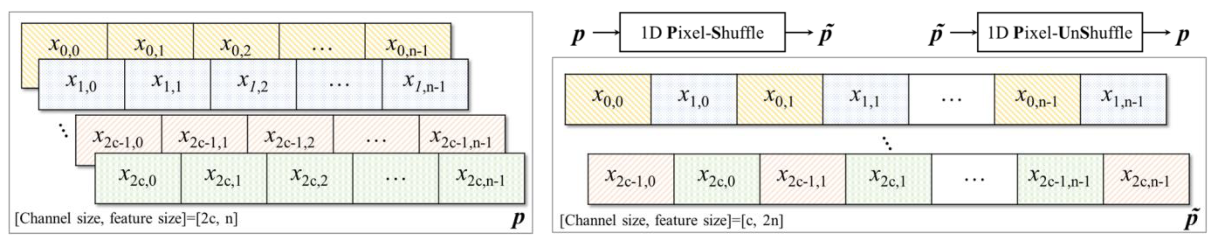
2.3. Pixel Shuffle (Subpixel)
3. Proposed CPDAE
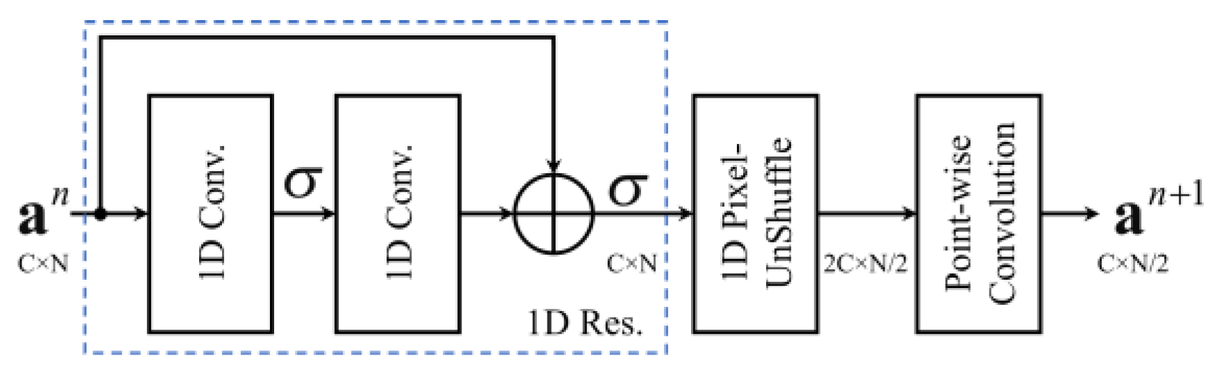
3.1. Encoder Layer
3.2. Channel-Wise Average Pooling in Skip Connection
3.3. Decoder Layer
4. Experimental Results
4.1. Evaluation Criteria
4.2. Dataset Selection and Experiment Preprocessing
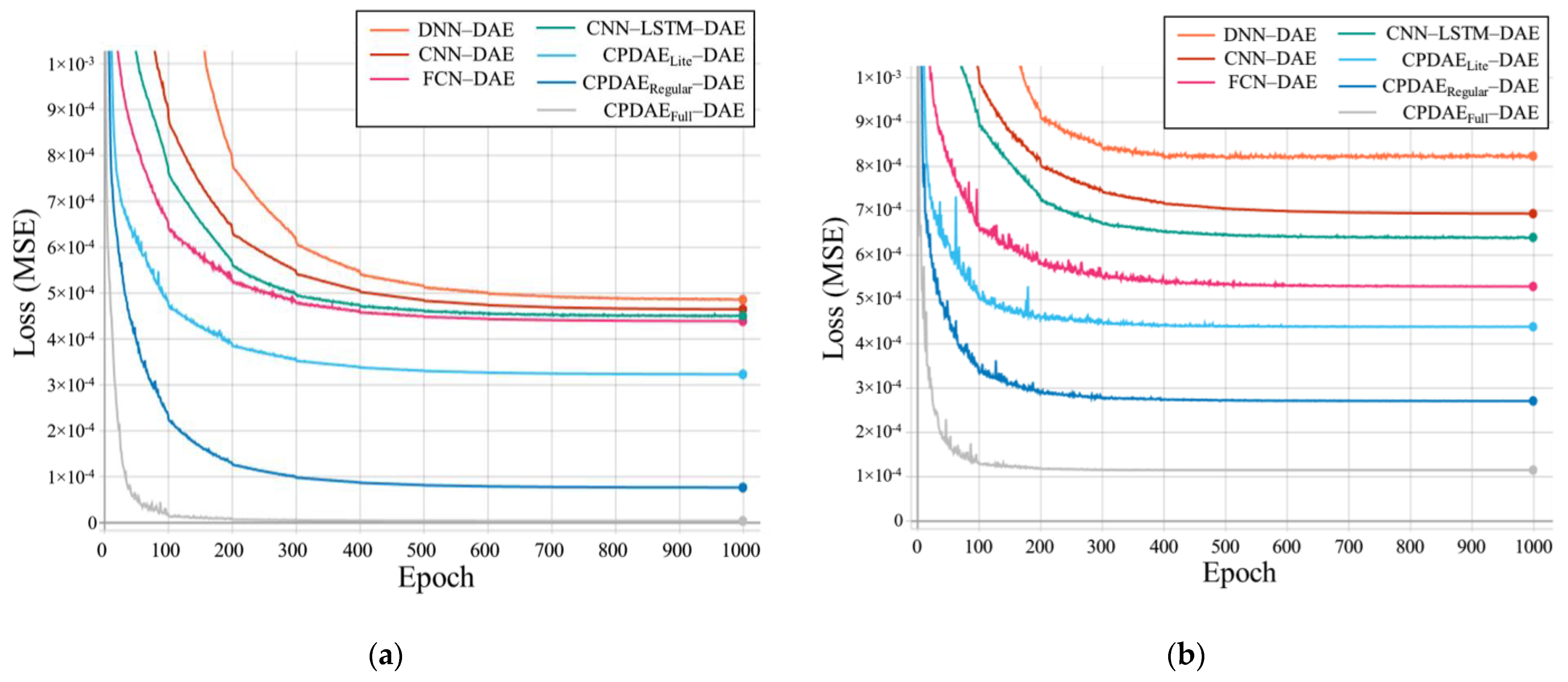
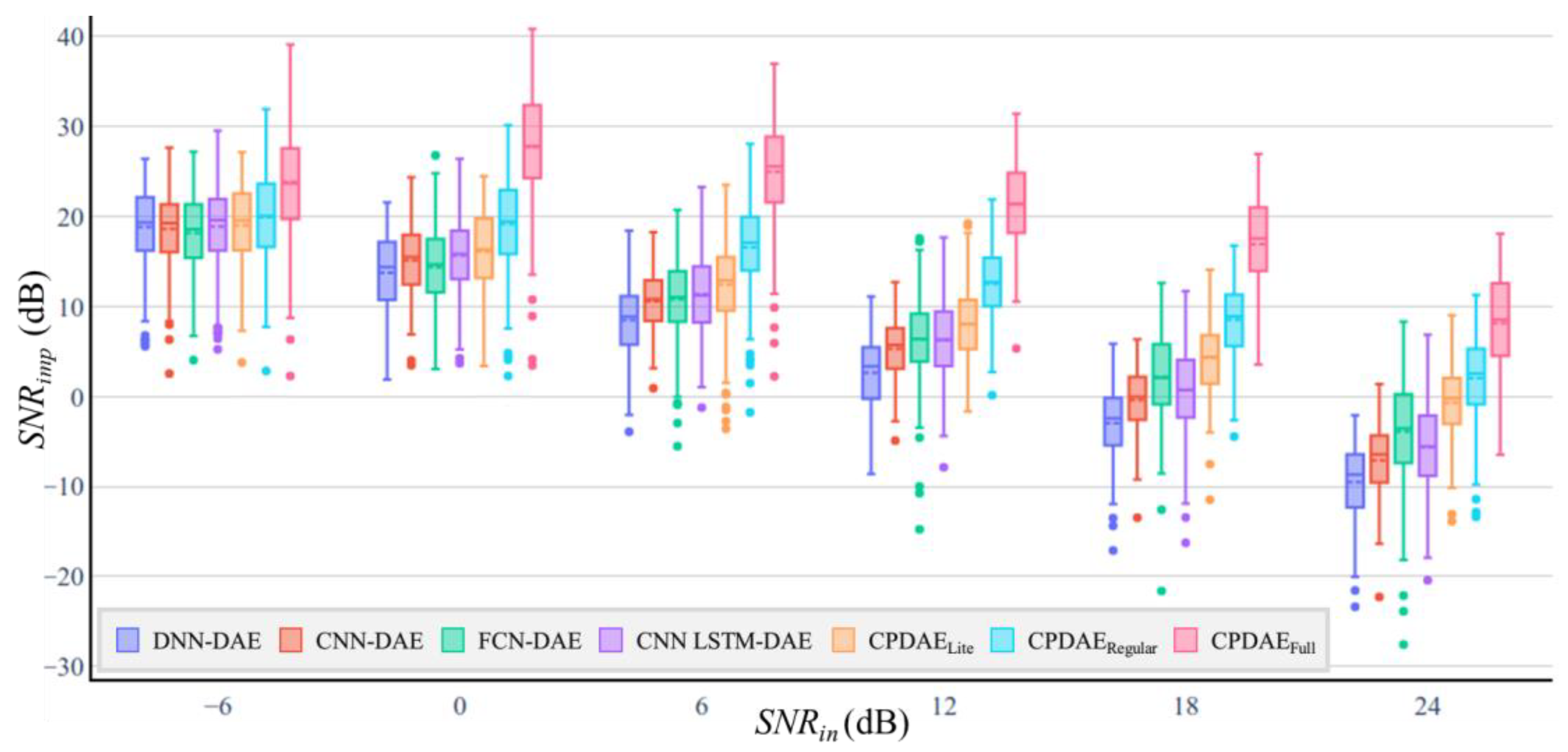
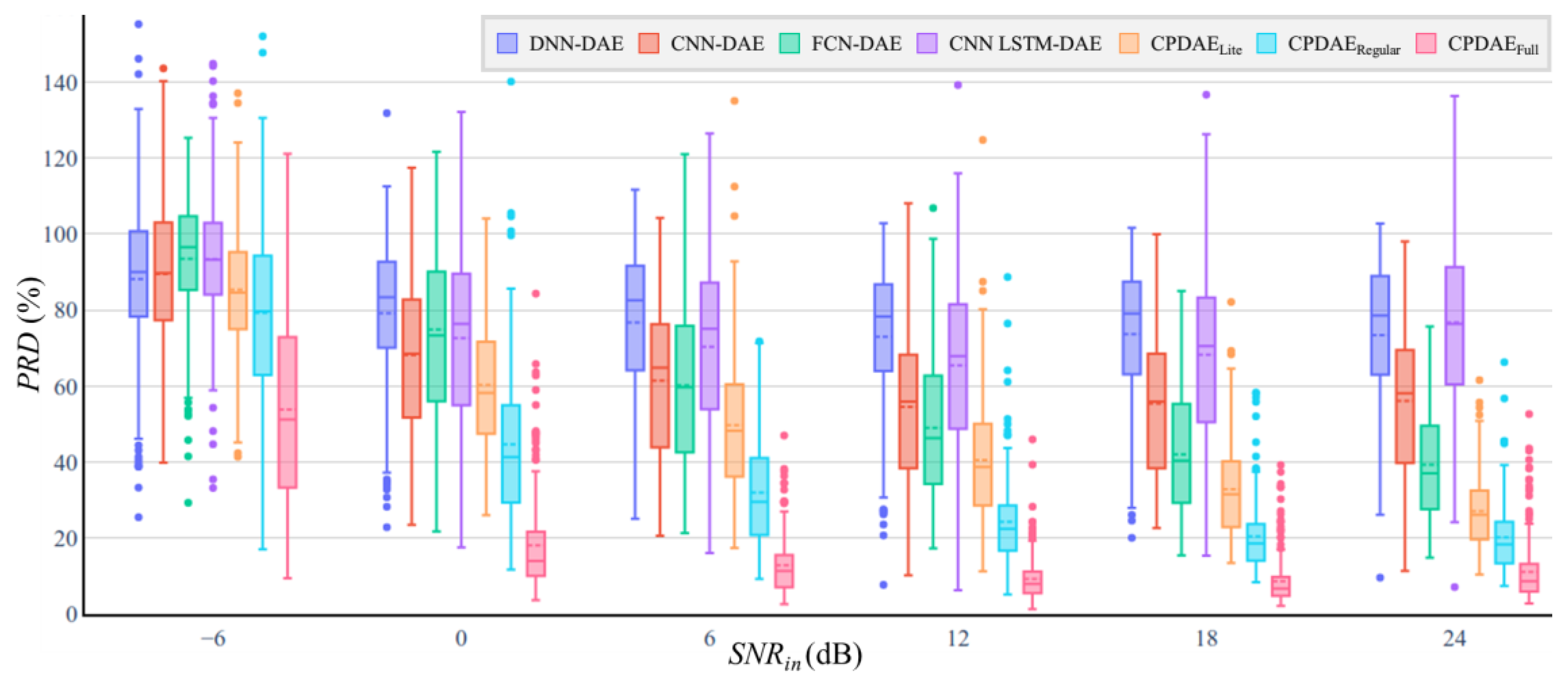
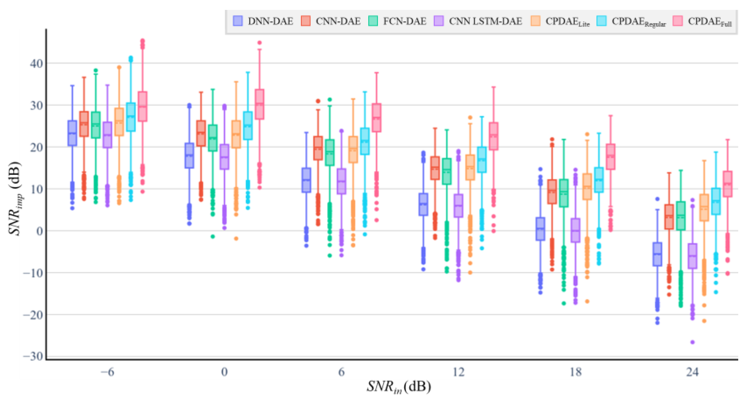
4.3. Experimental Results and Comparison
5. Conclusions
Supplementary Materials
Author Contributions
Funding
Informed Consent Statement
Data Availability Statement
Conflicts of Interest
References
- Roth, G.A.; Mensah, G.A.; Johnson, C.O.; Addolorato, G.; Ammirati, E.; Baddour, L.M.; Barengo, N.C.; Beaton, A.; Benjamin, E.J.; Benziger, C.P.; et al. Global Burden of Cardiovascular Diseases and Risk Factors, 1990–2019: Update from the GBD 2019 Study. J. Am. Coll. Cardiol. 2020, 76, 2982–3021. [Google Scholar] [CrossRef] [PubMed]
- Al-Khatib, S.M.; Stevenson, W.G.; Ackerman, M.J.; Bryant, W.J.; Callans, D.J.; Curtis, A.B.; Deal, B.J.; Dickfeld, T.; Field, M.E.; Fonarow, G.C.; et al. 2017 AHA/ACC/HRS Guideline for Management of Patients with Ventricular Arrhythmias and the Prevention of Sudden Cardiac Death. Circulation 2018, 138, e272–e391. [Google Scholar] [CrossRef] [PubMed] [Green Version]
- Salinet, J.L.; Luppi Silva, O. ECG Signal Acquisition Systems. In Developments and Applications for ECG Signal Processing: Modeling, Segmentation, and Pattern Recognition; Academic Press: Cambridge, MA, USA, 2019; pp. 29–51. [Google Scholar] [CrossRef]
- Sun, C.; Liao, J.; Wang, G.; Li, B.; Meng, M.Q.H. A portable 12-lead ECG acquisition system. In Proceedings of the 2013 IEEE International Conference on Information and Automation, ICIA, Yinchuan, China, 26–28 August 2013; pp. 368–373. [Google Scholar] [CrossRef]
- Webster, J.G. Reducing Motion Artifacts and Interference in Biopotential Recording. IEEE Trans. Biomed. Eng. 1984, BME-31, 823–826. [Google Scholar] [CrossRef]
- Huhta, J.C.; Webster, J.G. 60-Hz Interference in Electrocardiography. IEEE Trans. Biomed. Eng. 1973, BME-20, 91–101. [Google Scholar] [CrossRef] [PubMed]
- Lenis, G.; Pilia, N.; Loewe, A.; Schulze, W.H.W.; Dössel, O. Comparison of Baseline Wander Removal Techniques considering the Preservation of ST Changes in the Ischemic ECG: A Simulation Study. Comput. Math. Methods Med. 2017, 2017, 1–13. [Google Scholar] [CrossRef]
- Hesar, H.D.; Mohebbi, M. Muscle artifact cancellation in ECG signal using a dynamical model and particle filter. In Proceedings of the 2015 22nd Iranian Conference on Biomedical Engineering, ICBME 2015, Tehran, Iran, 25–27 November 2015; pp. 178–183. [Google Scholar] [CrossRef]
- Rahman, M.Z.U.; Shaik, R.A.; Reddy, D.V.R.K. Efficient and simplified adaptive noise cancelers for ecg sensor based remote health monitoring. IEEE Sens. J. 2012, 12, 566–573. [Google Scholar] [CrossRef]
- Rahman, M.Z.U.; Karthik, G.V.S.; Fathima, S.Y.; Lay-Ekuakille, A. An efficient cardiac signal enhancement using time–frequency realization of leaky adaptive noise cancelers for remote health monitoring systems. Measurement 2013, 46, 3815–3835. [Google Scholar] [CrossRef]
- Venkatesan, C.; Karthigaikumar, P.; Varatharajan, R. FPGA implementation of modified error normalized LMS adaptive filter for ECG noise removal. Clust. Comput. 2019, 22, 12233–12241. [Google Scholar] [CrossRef]
- Yadav, S.K.; Sinha, R.; Bora, P.K. Electrocardiogram signal denoising using non-local wavelet transform domain filtering. IET Signal Process. 2015, 9, 88–96. [Google Scholar] [CrossRef] [Green Version]
- Prashar, N.; Sood, M.; Jain, S. Design and implementation of a robust noise removal system in ECG signals using dual-tree complex wavelet transform. Biomed. Signal Process. Control 2021, 63, 102212. [Google Scholar] [CrossRef]
- Mourad, T. ECG Denoising Based on 1-D Double-Density Complex DWT and SBWT. In The Stationary Bionic Wavelet Transform and its Applications for ECG and Speech Processing; Mourad, T., Ed.; Springer International Publishing: Cham, Switzerland, 2022; pp. 31–50. ISBN 978-3-030-93405-7. [Google Scholar] [CrossRef]
- Lee, J.; McManus, D.D.; Merchant, S.; Chon, K.H. Automatic motion and noise artifact detection in holter ECG data using empirical mode decomposition and statistical approaches. IEEE Trans. Biomed. Eng. 2012, 59, 1499–1506. [Google Scholar] [CrossRef] [PubMed]
- Boda, S.; Mahadevappa, M.; Dutta, P.K. A hybrid method for removal of power line interference and baseline wander in ECG signals using EMD and EWT. Biomed. Signal Process. Control 2021, 67, 102466. [Google Scholar] [CrossRef]
- Patro, K.K.; Jaya Manmadha Rao, M.; Jadav, A.; Rajesh Kumar, P. Noise Removal in Long-Term ECG Signals Using EMD-Based Threshold Method. Lect. Notes Data Eng. Commun. Technol. 2021, 63, 461–469. [Google Scholar] [CrossRef]
- Blanco-Velasco, M.; Weng, B.; Barner, K.E. ECG signal denoising and baseline wander correction based on the empirical mode decomposition. Comput. Biol. Med. 2008, 38, 1–13. [Google Scholar] [CrossRef]
- Xiong, P.; Wang, H.; Liu, M.; Zhou, S.; Hou, Z.; Liu, X. ECG signal enhancement based on improved denoising auto-encoder. Eng. Appl. Artif. Intell. 2016, 52, 194–202. [Google Scholar] [CrossRef]
- Hao, H.; Liu, M.; Xiong, P.; Du, H.; Zhang, H.; Lin, F.; Hou, Z.; Liu, X. Multi-lead model-based ECG signal denoising by guided filter. Eng. Appl. Artif. Intell. 2019, 79, 34–44. [Google Scholar] [CrossRef]
- Xiong, P.; Wang, H.; Liu, M.; Liu, X. Denoising autoencoder for eletrocardiogram signal enhancement. J. Med. Imaging Health Inform. 2015, 5, 1804–1810. [Google Scholar] [CrossRef]
- Chiang, H.T.; Hsieh, Y.Y.; Fu, S.W.; Hung, K.H.; Tsao, Y.; Chien, S.Y. Noise Reduction in ECG Signals Using Fully Convolutional Denoising Autoencoders. IEEE Access 2019, 7, 60806–60813. [Google Scholar] [CrossRef]
- Dasan, E.; Panneerselvam, I. A novel dimensionality reduction approach for ECG signal via convolutional denoising autoencoder with LSTM. Biomed. Signal Process. Control 2021, 63, 102225. [Google Scholar] [CrossRef]
- El Bouny, L.; Khalil, M.; Adib, A. Convolutional Denoising Auto-Encoder Based AWGN Removal from ECG Signal. In Proceedings of the 2021 International Conference on INnovations in Intelligent SysTems and Applications, INISTA 2021, Kocaeli, Turkey, 25–27 August 2021. [Google Scholar]
- Bing, P.; Liu, W.; Zhang, Z. DeepCEDNet: An Efficient Deep Convolutional Encoder-Decoder Networks for ECG Signal Enhancement. IEEE Access 2021, 9, 56699–56708. [Google Scholar] [CrossRef]
- Nurmaini, S.; Darmawahyuni, A.; Sakti Mukti, A.N.; Rachmatullah, M.N.; Firdaus, F.; Tutuko, B.; Mukti, A.N.S.; Rachmatullah, M.N.; Firdaus, F.; Tutuko, B. Deep Learning-Based Stacked Denoising and Autoencoder for ECG Heartbeat Classification. Electronics 2020, 9, 135. [Google Scholar] [CrossRef] [Green Version]
- Wang, G.; Yang, L.; Liu, M.; Yuan, X.; Xiong, P.; Lin, F.; Liu, X. ECG signal denoising based on deep factor analysis. Biomed. Signal Process. Control 2020, 57, 101824. [Google Scholar] [CrossRef]
- He, Z.; Liu, X.; He, H.; Wang, H. Dual Attention Convolutional Neural Network Based on Adaptive Parametric ReLU for Denoising ECG Signals with Strong Noise. In Proceedings of the 2021 43rd Annual International Conference of the IEEE Engineering in Medicine & Biology Society (EMBC), Guadalajara, Mexico, 1–5 November 2021; pp. 779–782. [Google Scholar]
- Huang, N.E.; Shen, Z.; Long, S.R.; Wu, M.C.; Snin, H.H.; Zheng, Q.; Yen, N.C.; Tung, C.C.; Liu, H.H. The empirical mode decomposition and the Hilbert spectrum for nonlinear and non-stationary time series analysis. Proc. R. Soc. Lond. Ser. A Math. Phys. Eng. Sci. 1998, 454, 903–995. [Google Scholar] [CrossRef]
- Moody, G.B.; Mark, R.G. The impact of the MIT-BIH arrhythmia database. IEEE Eng. Med. Biol. Mag. 2001, 20, 45–50. [Google Scholar] [CrossRef]
- George, M.; Warren, M.; Roger, M. A noise stress test for arrhythmia detectors. Comput. Cardiol. 1984, 11, 381–384. [Google Scholar]
- Singh, P.; Pradhan, G. A New ECG Denoising Framework Using Generative Adversarial Network. IEEE/ACM Trans. Comput. Biol. Bioinform. 2021, 18, 759–764. [Google Scholar] [CrossRef]
- Goldberger, A.L.; Amaral, L.A.; Glass, L.; Hausdorff, J.M.; Ivanov, P.C.; Mark, R.G.; Mietus, J.E.; Moody, G.B.; Peng, C.K.; Stanley, H.E. PhysioBank, PhysioToolkit, and PhysioNet. Circulation 2000, 101, e215–e220. [Google Scholar] [CrossRef] [Green Version]
- Liu, J.Y.; Yang, Y.H. Denoising Auto-Encoder with Recurrent Skip Connections and Residual Regression for Music Source Separation. In Proceedings of the 17th IEEE International Conference on Machine Learning and Applications, ICMLA 2018, Orlando, FL, USA, 17–20 December 2018; pp. 773–778. [Google Scholar] [CrossRef] [Green Version]
- Peng, Y.; Zhang, L.; Liu, S.; Wu, X.; Zhang, Y.; Wang, X. Dilated Residual Networks with Symmetric Skip Connection for image denoising. Neurocomputing 2019, 345, 67–76. [Google Scholar] [CrossRef]
- Dong, L.F.; Gan, Y.Z.; Mao, X.L.; Yang, Y.B.; Shen, C. Learning Deep Representations Using Convolutional Auto-encoders with Symmetric Skip Connections. In Proceedings of the ICASSP, IEEE International Conference on Acoustics, Speech and Signal Processing, Calgary, AB, Canada, 15–20 April 2018; pp. 3006–3010. [Google Scholar] [CrossRef] [Green Version]
- Liu, T.; Wang, J.; Liu, Q.; Alibhai, S.; Lu, T. High-Ratio Lossy Compression: Exploring the Autoencoder to Compress Scientific Data; High-Ratio Lossy Compression: Exploring the Autoencoder to Compress Scientific Data. IEEE Trans. Big Data 2021, PP, 2332–7790. [Google Scholar] [CrossRef]
- Vincent, P.; Larochelle, H.; Bengio, Y.; Manzagol, P.A. Extracting and composing robust features with denoising autoencoders. In Proceedings of the 25th International Conference on Machine Learning, Helsinki, Finland, 5–9 July 2008; pp. 1096–1103. [Google Scholar] [CrossRef] [Green Version]
- Lee, D.; Choi, S.; Kim, H.J. Performance evaluation of image denoising developed using convolutional denoising autoencoders in chest radiography. Nucl. Instrum. Methods Phys. Res. Sect. A Accel. Spectrometers Detect. Assoc. Equip. 2018, 884, 97–104. [Google Scholar] [CrossRef]
- Lu, X.; Tsao, Y.; Matsuda, S.; Hori, C. Speech enhancement based on deep denoising autoencoder. In Proceedings of the Annual Conference of the International Speech Communication Association, Interspeech, Lyon, France, 25–29 August 2013; pp. 436–440. [Google Scholar] [CrossRef]
- He, K.; Zhang, X.; Ren, S.; Sun, J. Deep Residual Learning for Image Recognition. In Proceedings of the IEEE Computer Society Conference on Computer Vision and Pattern Recognition, Las Vegas, NV, USA, 27–30 June 2016; pp. 770–778. [Google Scholar] [CrossRef] [Green Version]
- Werbos, P. Beyond Regression: New Tools for Prediction and Analysis in the Behavioral Science. Ph.D. Thesis, Harvard University, Cambridge, MA, USA, 1974. [Google Scholar]
- Shi, W.; Caballero, J.; Huszar, F.; Totz, J.; Aitken, A.P.; Bishop, R.; Rueckert, D.; Wang, Z. Real-Time Single Image and Video Super-Resolution Using an Efficient Sub-Pixel Convolutional Neural Network. In Proceedings of the IEEE Computer Society Conference on Computer Vision and Pattern Recognition, Las Vegas, NV, USA, 27–30 June 2016; pp. 1874–1883. [Google Scholar] [CrossRef] [Green Version]
- Aitken, A.; Ledig, C.; Theis, L.; Caballero, J.; Wang, Z.; Shi, W. Checkerboard artifact free sub-pixel convolution: A note on sub-pixel convolution, resize convolution and convolution resize. arXiv 2017, arXiv:1707.02937. [Google Scholar]
- Chollet, F. Xception: Deep Learning with Depthwise Separable Convolutions. In Proceedings of the 30th IEEE Conference on Computer Vision and Pattern Recognition, CVPR 2017, Honolulu, HI, USA, 21–26 July 2017; pp. 1800–1807. [Google Scholar] [CrossRef] [Green Version]
- Hascoet, T.; Zhuang, W.; Febvre, Q.; Ariki, Y.; Takiguchi, T.; Hascoet, T.; Zhuang, W.; Febvre, Q.; Ariki, Y.; Takiguchi, T. Reducing the Memory Cost of Training Convolutional Neural Networks by CPU Offloading. J. Softw. Eng. Appl. 2019, 12, 307–320. [Google Scholar] [CrossRef]
- Němcová, A.; Smíšek, R.; Maršánová, L.; Smital, L.; Vítek, M. A comparative analysis of methods for evaluation of ECG signal quality after compression. BioMed Res. Int. 2018, 2018, 1–26. [Google Scholar] [CrossRef] [PubMed]
- Luz, E.J.d.S.; Schwartz, W.R.; Cámara-Chávez, G.; Menotti, D. ECG-based heartbeat classification for arrhythmia detection: A survey. Comput. Methods Programs Biomed. 2016, 127, 144–164. [Google Scholar] [CrossRef] [PubMed]
- Moody, G.; Mark, R. MIT-BIH Noise Stress Test Database v1.0.0. Available online: https://physionet.org/content/nstdb/1.0.0/ (accessed on 1 February 2020).
- Moody, G.; Mark, R. MIT-BIH Arrhythmia Database v1.0.0. Available online: https://physionet.org/content/mitdb/1.0.0/ (accessed on 1 February 2020).
- Senior, A.; Heigold, G.; Ranzato, M.; Yang, K. An empirical study of learning rates in deep neural networks for speech recognition. In Proceedings of the ICASSP, IEEE International Conference on Acoustics, Speech and Signal Processing, Vancouver, BC, Canada, 26–31 May 2013; pp. 6724–6728. [Google Scholar]
- Moody, G.; Mark, R. MIT-BIH Normal Sinus Rhythm Database v1.0.0. Available online: https://physionet.org/content/nsrdb/1.0.0/ (accessed on 1 February 2020).


| Methods | Advantage | Disadvantage |
|---|---|---|
| Adaptive Filter [9,10,11] | (1) Simplest and easy to implement on embedded systems or digital signal processors. (2) Compared with AI algorithms, it has less computational complexity. (3) The category can be time domain and frequency domain processing. | (1) A noise signal as a reference signal is requested, and different noise sources would generate different weights, which cannot be shared. (2) The system would fail to work if the noise of the external environment changes suddenly and the weight updates too slow. |
| DWT-DAE [12,13,14] | (1) It can extract the feature in the spatial domain and has an effectively computational ability. (2) It takes more computational complexity than adaptive filter approaches but gains better results. | (1) It is very hard to definite the value of the software and hardware thresholds for all scenarios. (2) The selection of mother wavelet functions would generate different results. |
| EMD [15,16,17,18] | (1) Baseline wander can be easily removed by using the highest IMF. (2) The process of the EMD algorithm is simple and routine so it is not suitable for complex and varied noises. | (1) The IMFs of noise may contain some part of ECG feature that cannot be arbitrarily discarded. (2) The EMD algorithm takes the amount of computing time for the routine process and cannot be real-time and online executed due to the data dependency of IMFs’ calculations. |
| Execution Order-Annotation | Type | 1D NN Layer Name | No. Filter × Kernel Size | Paddings | Region/Unit Size | * AF | No. Trainable Parameter | Output Size |
|---|---|---|---|---|---|---|---|---|
| 0-Input () | Noisy ECG | 1 × 1024 | ||||||
| 1 | Input Layer | Convolution | 32 × 1 | 0 | – | – | 64 | 32 × 1024 |
| 2 | Res. | 32 × 5 | 2 | ↓ 2 | ReLU | 10,304 | 32 × 1024 | |
| 3 | Encoder Layer 1 | Res. + PUS + PW Conv. | 32 × 5 | 2 | ↓ 2 | ReLU | 12,384 | 32 × 512 |
| 5 | Encoder Layer 2 | Res. + PUS + PW Conv. | 32 × 5 | 2 | ↓ 2 | ReLU | 12,384 | 32 × 256 |
| 7 | Encoder Layer 3 | Res. + PUS + PW Conv. | 32 × 5 | 2 | ↓ 2 | ReLU | 12,384 | 32 × 128 |
| 9 | Encoder Layer 4 | Res. + PUS + PW Conv. | 32 × 5 | 2 | ↓ 2 | ReLU | 12,384 | 32 × 64 |
| 11 | Encoder Layer 5 | Res. + PUS + PW Conv. | 32 × 5 | 2 | ↓ 2 | ReLU | 12,384 | 32 × 32 |
| 13 | Encoder Layer 6 | Res. + PUS + PW Conv. | 32 × 5 | 2 | ↓ 2 | ReLU | 12,384 | 32 × 16 |
| 15-Code (z) | Encoder Layer 7 | Res. + PUS + PW Conv. | 32 × 5 | 2 | ↓ 2 | ReLU | 12,384 | 32×8 |
| 16 | Decoder Layer 7 | Res. + PW Conv. + PS | 32 × 5 | 2 | ↑ 2 | ReLU | 12,416 | 32 × 16 |
| 17 | Decoder Layer 6 | Res. + PW Conv. + PS | 32 × 5 | 2 | ↑ 2 | ReLU | 12,416 | 32 × 32 |
| 18 | Decoder Layer 5 | Res. + PW Conv. + PS | 32 × 5 | 2 | ↑ 2 | ReLU | 12,416 | 32 × 64 |
| 19 | Decoder Layer 4 | Res. + PW Conv. + PS | 32 × 5 | 2 | ↑ 2 | ReLU | 12,416 | 32 × 128 |
| 20 | Decoder Layer 3 | Res. + PW Conv. + PS | 32 × 5 | 2 | ↑ 2 | ReLU | 12,416 | 32 × 256 |
| 21 | Decoder Layer 2 | Res. + PW Conv. + PS | 32 × 5 | 2 | ↑ 2 | ReLU | 12,416 | 32 × 512 |
| 22 | Decoder Layer 1 | Res. + PW Conv. + PS | 32 × 5 | 2 | ↑ 2 | ReLU | 12,416 | 32 × 1024 |
| 23 | Output Layer | Res. | 32 × 5 | 2 | ↓ 2 | ReLU | 10,304 | 32 × 1024 |
| 24 | Convolution | 32 × 1 | 0 | – | – | 33 | 1 × 1024 | |
| 25-Output () | Reconstructed ECG | 1 × 1024 | ||||||
| 4-En. 1→De.1 | CWAP & PW Conv. #1 | CWAP + PW Conv. | 32 × 1 | 0 | – | – | 64 | 32 × 16 |
| 6-En. 2→De.2 | CWAP & PW Conv. #2 | CWAP + PW Conv. | 32 × 1 | 0 | – | – | 64 | 32 × 32 |
| 8-En. 3→De.3 | CWAP & PW Conv. #3 | CWAP + PW Conv. | 32 × 1 | 0 | – | – | 64 | 32 × 64 |
| 10-En. 4→De.4 | CWAP & PW Conv. #4 | CWAP + PW Conv. | 32 × 1 | 0 | – | – | 64 | 32 × 128 |
| 12-En. 5→De.5 | CWAP & PW Conv. #5 | CWAP + PW Conv. | 32 × 1 | 0 | – | – | 64 | 32 × 256 |
| 14-En. 6→De.6 | CWAP & PW Conv. #6 | CWAP + PW Conv. | 32 × 1 | 0 | – | – | 64 | 32 × 512 |
| Total parameters: 194,689 | Total MACs: 56.96 M | Forward/Backward memory size: 4.44 Mbytes | ||||||
| Execution Order-Annotation | 1D NN Layer Name | No. Filter × Kernel Size | Paddings | Region/Unit Size | * AF | No. Trainable Parameter (w, b) | Input Size | Output Size |
|---|---|---|---|---|---|---|---|---|
| Residual Block (Res.) | 10,304 | 32 × N | 32 × N | |||||
| 1-Conv. | Convolution | 32 × 5 | 2 | – | – | 5152 | 32 × N | 32 × N |
| 2-Conv. | Convolution | 32 × 5 | 2 | – | ReLU | 5152 | 32 × N | 32 × N |
| Encoder Layer (Res. + PUS + PW Conv.) | 12,384 | 32 × N | 32 × N/2 | |||||
| 1-Res. | Residual Block | 32 × 5 | 2 | – | ReLU | 10,304 | 32 × N | 32 × N |
| 2-PUS | Pixel-UnShuffle | – | – | ↓ 2 | – | – | 32 × N | 64 × N/2 |
| 3-PW Conv. | Convolution | 32 × 1 | 0 | – | – | 2080 | 64 × N/2 | 32 × N/2 |
| Decoder Layer (Res. + PW Conv. + PS) | 12,416 | 32 × N | 32 × 2N | |||||
| 1-Res. | Residual Block | 32 × 5 | 2 | – | – | 10,304 | 32 × N | 32 × N |
| 2-PW Conv. | Convolution | 64 × 1 | 0 | – | ReLU | 2112 | 32 × N | 64 × N |
| 3-PS | Pixel-Shuffle | – | – | ↑ 2 | – | – | 64 × N | 32 × 2N |
| Skip Connection (CWAP + PW Conv.) | 64 | 32 × N | 32 × N | |||||
| 1-CWAP | Channel-wise Average Pooling | – | – | ↓ 32 | – | – | 32 × N | 1 × N |
| 2-PW Conv. | Convolution | 32 × 1 | 0 | ↑ 32 | – | 64 | 1 × N | 32 × N |
| Hyperparameters | Value |
|---|---|
| Cost function | Mean-square-error (MSE) |
| Learning Rate (LR) | 1 × 10⁻⁴ |
| Learning Rate scheduler | Step-LR () |
| Optimizer | Adam |
| Batch size | 32 |
| Epochs | 1000 |
| Proposed Models | No. Encoder/Decoder Layers | No. Channels | Kernel Size | MACs | Average Run-Time (ms) per Frame | |
|---|---|---|---|---|---|---|
| Training Phase | Testing Phase | |||||
| CPDAELite | 8 | 16 | 5 | 14.69 M | 0.5508 | 0.1154 |
| CPDAERegular | 7 | 32 | 5 | 56.96 M | 0.6439 | 0.1424 |
| CPDAEFull | 6 | 128 | 5 | 355.01 M | 0.6935 | 0.1327 |
| DAE Model | Number of Trainable Parameters | MACs | SNRimp (dB) | PRD (%) | ||||||||||
|---|---|---|---|---|---|---|---|---|---|---|---|---|---|---|
| SNRin −6 dB | SNRin 0 dB | SNRin 6 dB | SNRin 12 dB | SNRin 18 dB | SNRin 24 dB | SNRin −6 dB | SNRin 0 dB | SNRin 6 dB | SNRin 12 dB | SNRin 18 dB | SNRin 24 dB | |||
| DNN | 1,399,712 | 1.4 M | 18.83 | 13.72 | 8.49 | 2.62 | −2.94 | −9.5 | 88.15 | 79.13 | 76.70 | 73.00 | 73.65 | 73.38 |
| CNN | 1,116,478 | 13.27 M | 18.63 | 15.11 | 10.58 | 5.29 | −0.36 | −7.08 | 89.45 | 68.19 | 61.41 | 54.50 | 55.38 | 56.09 |
| FCN [22] | 78,444 | 25.08 M | 18.60 | 14.38 | 10.80 | 6.35 | 2.18 | −3.88 | 93.53 | 73.29 | 60.21 | 49.00 | 42.01 | 39.29 |
| CNN-LSTM [23] | 10,920,532 | 46.69 M | 18.90 | 15.66 | 11.24 | 6.25 | 0.73 | −5.63 | 86.92 | 65.23 | 54.68 | 42.70 | 47.44 | 47.38 |
| CPDAELite | 55,505 | 14.43 M | 18.85 | 16.12 | 12.44 | 8.01 | 4.31 | −0.72 | 84.60 | 58.17 | 49.72 | 40.51 | 32.87 | 27.05 |
| CPDAERegular | 194,689 | 56.96 M | 19.91 | 19.18 | 16.60 | 12.55 | 8.52 | 2.03 | 79.26 | 44.66 | 31.99 | 24.26 | 20.45 | 20.23 |
| CPDAEFull | 2,694,529 | 355.01 M | 23.68 | 27.75 | 24.99 | 21.38 | 16.92 | 8.15 | 51.20 | 18.10 | 12.81 | 9.28 | 8.65 | 8.66 |
Publisher’s Note: MDPI stays neutral with regard to jurisdictional claims in published maps and institutional affiliations. |
© 2022 by the authors. Licensee MDPI, Basel, Switzerland. This article is an open access article distributed under the terms and conditions of the Creative Commons Attribution (CC BY) license (https://creativecommons.org/licenses/by/4.0/).
Share and Cite
Jhang, Y.-S.; Wang, S.-T.; Sheu, M.-H.; Wang, S.-H.; Lai, S.-C. Channel-Wise Average Pooling and 1D Pixel-Shuffle Denoising Autoencoder for Electrode Motion Artifact Removal in ECG. Appl. Sci. 2022, 12, 6957. https://doi.org/10.3390/app12146957
Jhang Y-S, Wang S-T, Sheu M-H, Wang S-H, Lai S-C. Channel-Wise Average Pooling and 1D Pixel-Shuffle Denoising Autoencoder for Electrode Motion Artifact Removal in ECG. Applied Sciences. 2022; 12(14):6957. https://doi.org/10.3390/app12146957
Chicago/Turabian StyleJhang, Yu-Syuan, Szu-Ting Wang, Ming-Hwa Sheu, Szu-Hong Wang, and Shin-Chi Lai. 2022. "Channel-Wise Average Pooling and 1D Pixel-Shuffle Denoising Autoencoder for Electrode Motion Artifact Removal in ECG" Applied Sciences 12, no. 14: 6957. https://doi.org/10.3390/app12146957
APA StyleJhang, Y.-S., Wang, S.-T., Sheu, M.-H., Wang, S.-H., & Lai, S.-C. (2022). Channel-Wise Average Pooling and 1D Pixel-Shuffle Denoising Autoencoder for Electrode Motion Artifact Removal in ECG. Applied Sciences, 12(14), 6957. https://doi.org/10.3390/app12146957