
SBNN: A Searched Binary Neural Network for SAR Ship Classification

Abstract
:1. Introduction
2. Related Work
2.1. Network Architecture Search
2.2. Binary Network
2.3. Spatial Information Processing
3. SBNN
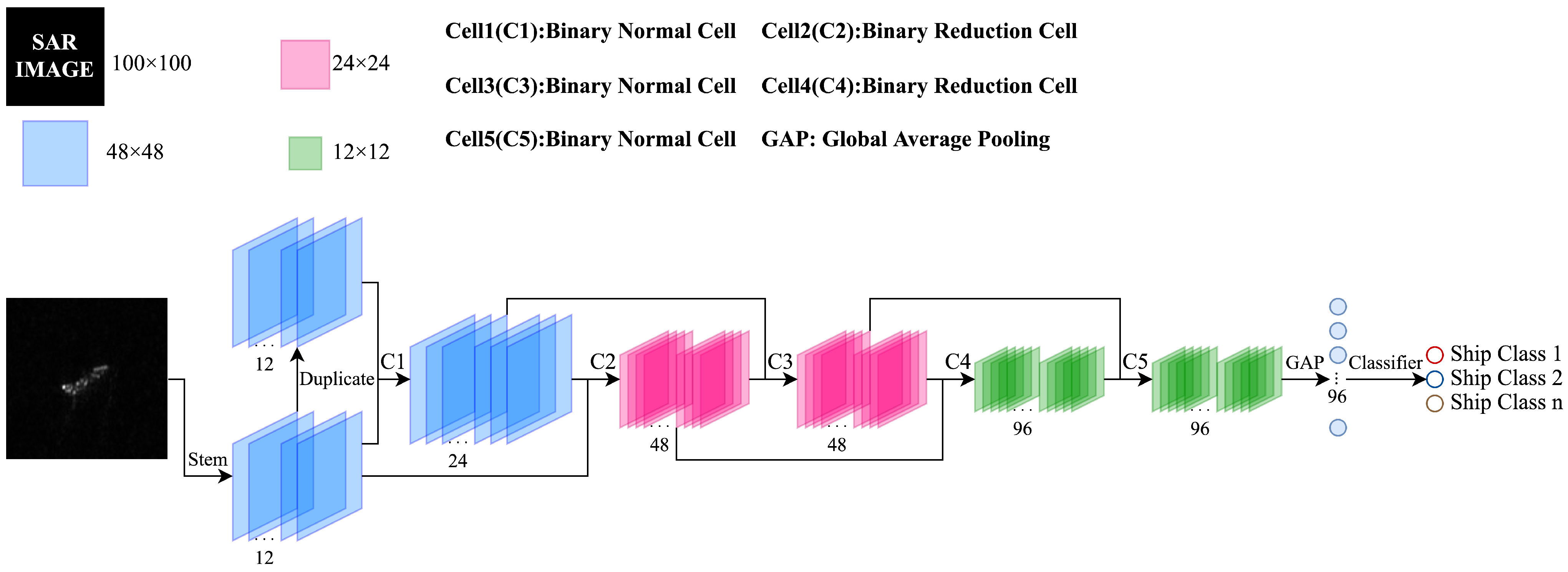
3.1. Overall Network Architecture
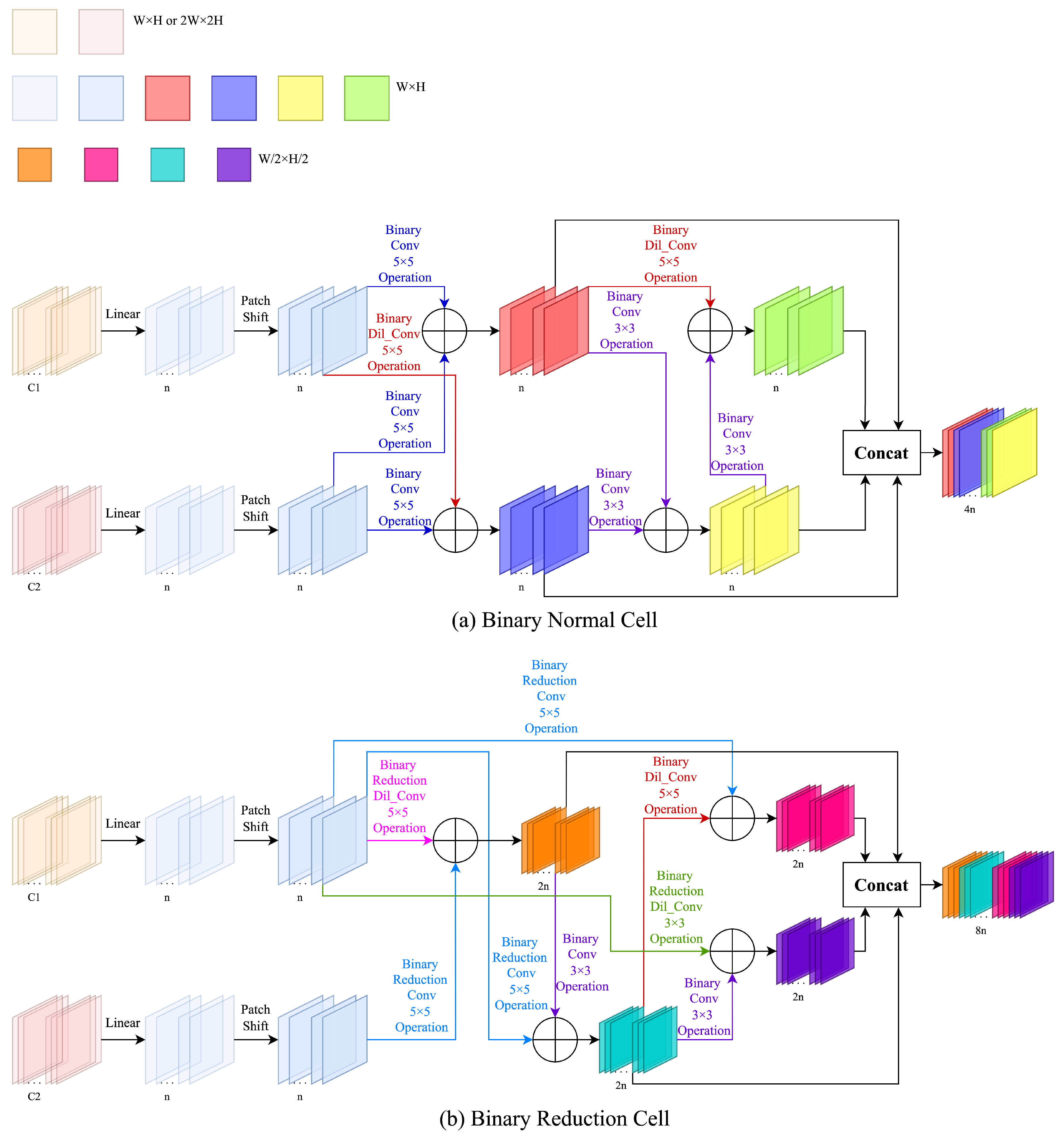
3.2. Searched Normal Cell and Reduction Cell
3.2.1. Efficient Searching
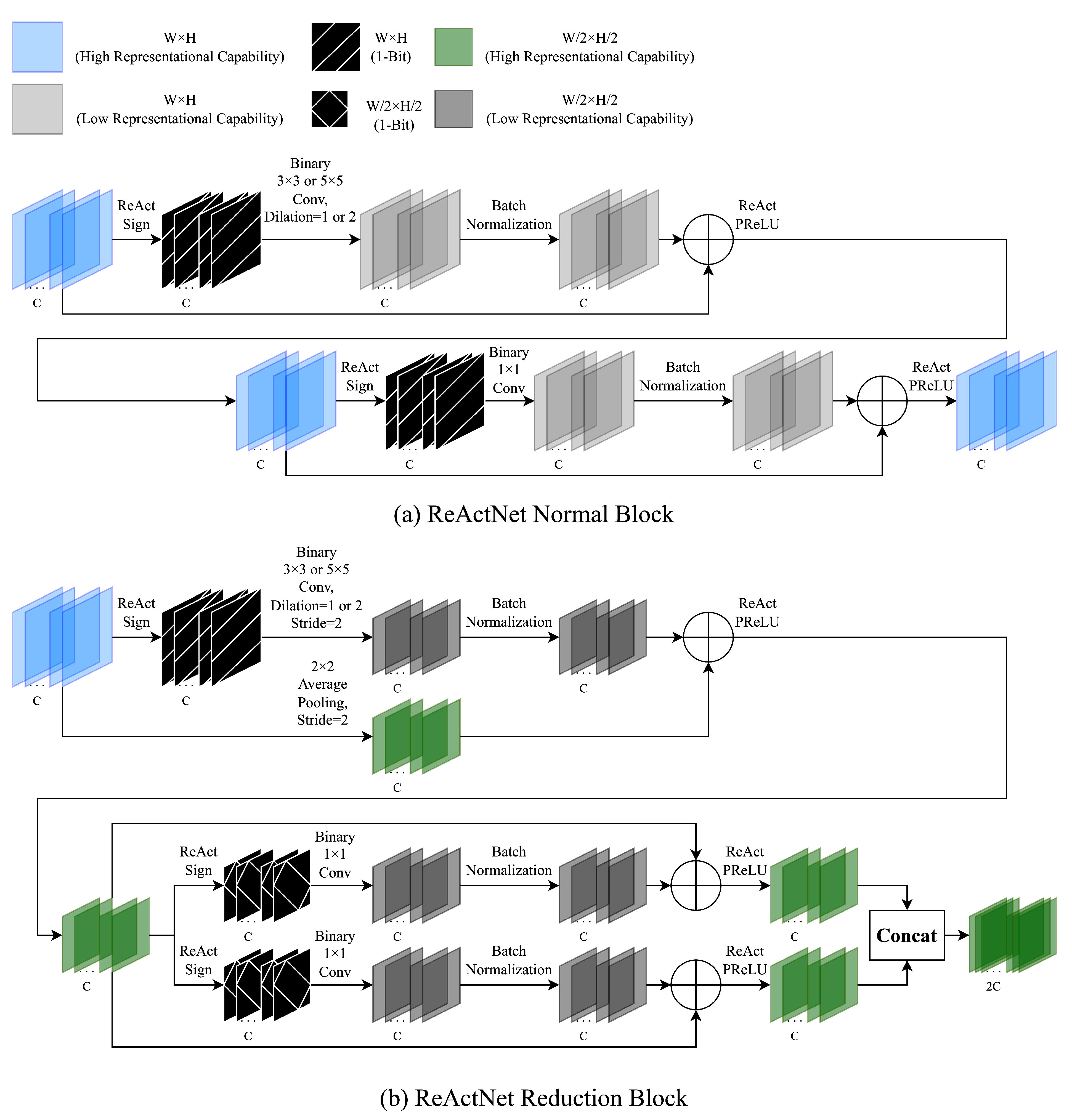
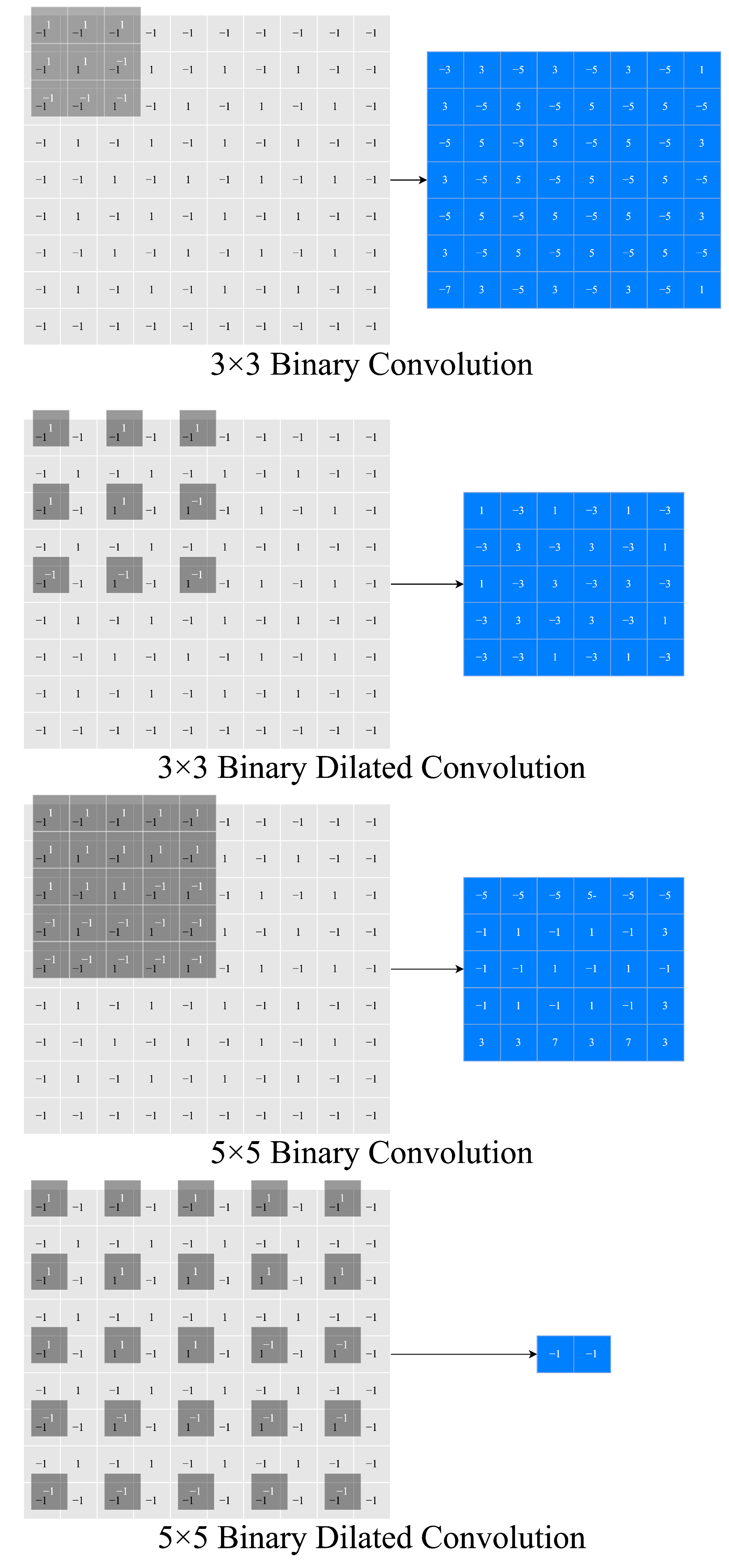
3.2.2. Modification and Binarization
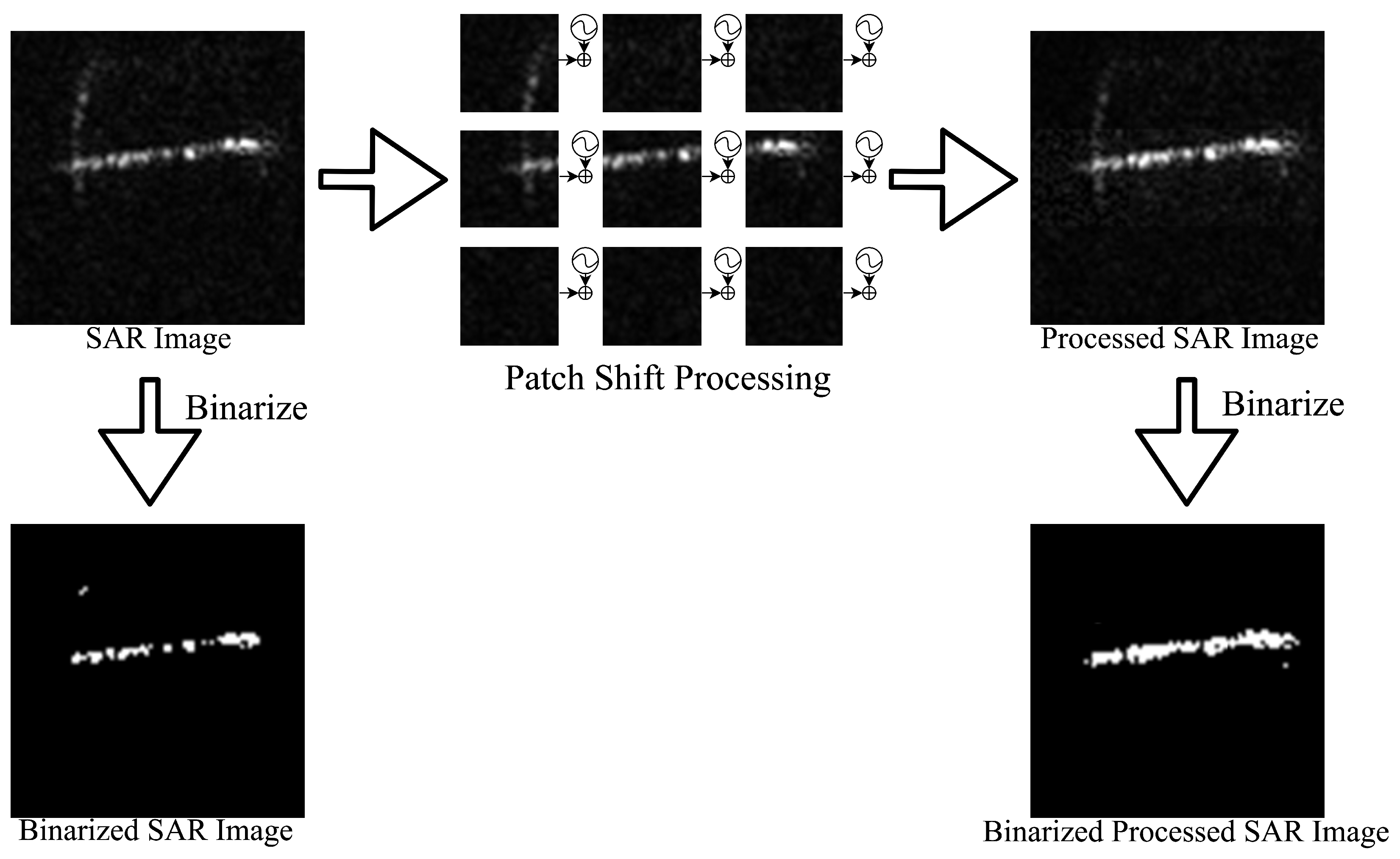
3.2.3. Patch Shift Processing
4. Experiments
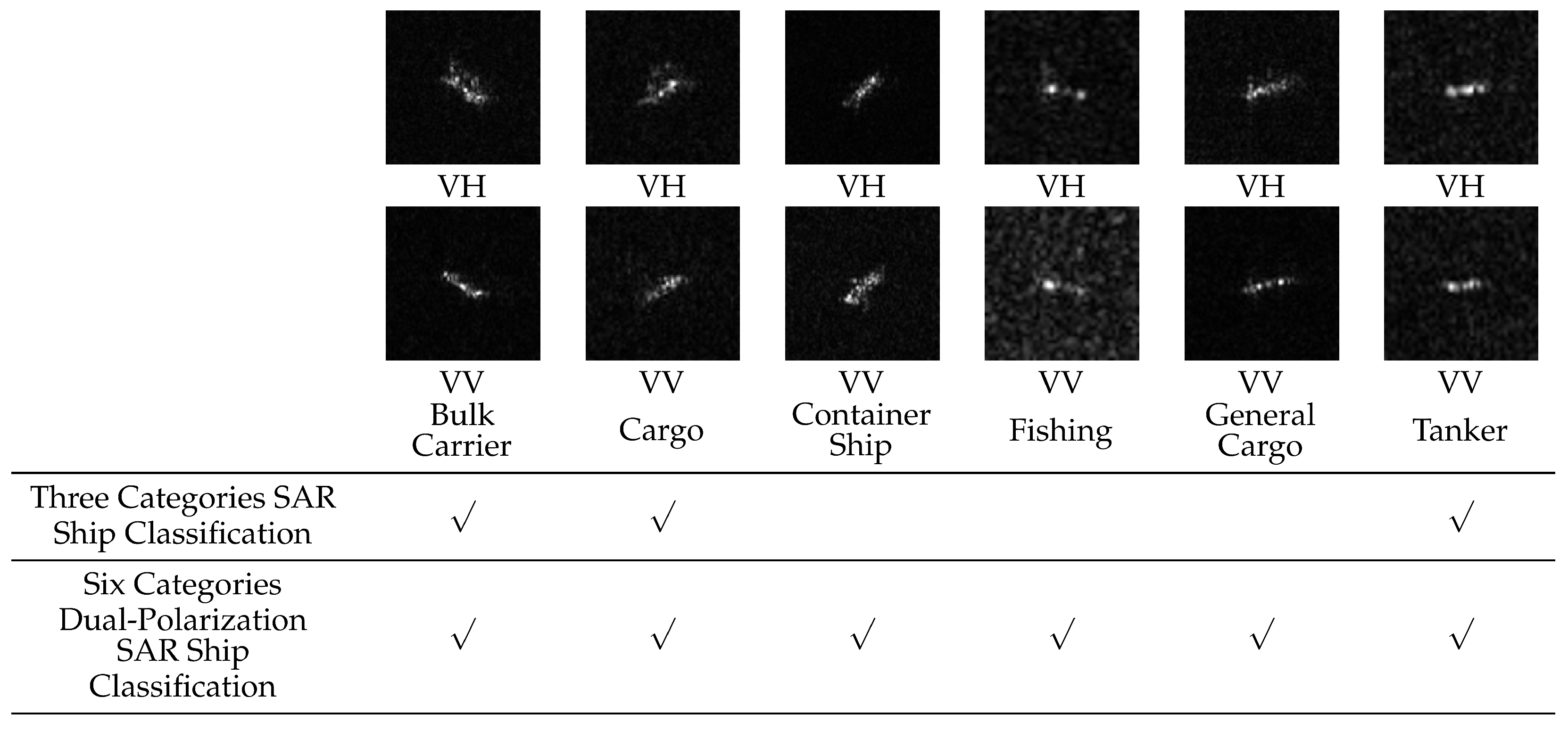
4.1. Dataset
4.2. Experimental Details
4.2.1. Trainning
4.2.2. Inferring
4.3. Results
4.3.1. Comparison with CNN-Based SAR Ship Classification Methods
4.3.2. Comparison with Modern Computer Vision Binary Networks
4.4. Ablation Study
4.4.1. Candidate Operations
4.4.2. Patch Shift Processing
5. Conclusions
Author Contributions
Funding
Institutional Review Board Statement
Informed Consent Statement
Data Availability Statement
Acknowledgments
Conflicts of Interest
References
- Brusch, S.; Lehner, S.; Fritz, T.; Soccorsi, M.; Soloviev, A.; van Schie, B. Ship surveillance with TerraSAR-X. IEEE Trans. Geosci. Remote Sens. 2010, 49, 1092–1103. [Google Scholar] [CrossRef]
- Petit, M.; Stretta, J.M.; Farrugio, H.; Wadsworth, A. Synthetic aperture radar imaging of sea surface life and fishing activities. IEEE Trans. Geosci. Remote Sens. 1992, 30, 1085–1089. [Google Scholar] [CrossRef] [Green Version]
- Park, J.; Lee, J.; Seto, K.; Hochberg, T.; Wong, B.A.; Miller, N.A.; Takasaki, K.; Kubota, H.; Oozeki, Y.; Doshi, S.; et al. Illuminating dark fishing fleets in North Korea. Sci. Adv. 2020, 6, eabb1197. [Google Scholar] [CrossRef]
- Cortes, C.; Vapnik, V. Support-vector networks. Mach. Learn. 1995, 20, 273–297. [Google Scholar] [CrossRef]
- Quinlan, J.R. Induction of decision trees. Mach. Learn. 1986, 1, 81–106. [Google Scholar] [CrossRef] [Green Version]
- Ho, T.K. The random subspace method for constructing decision forests. IEEE Trans. Pattern Anal. Mach. Intell. 1998, 20, 832–844. [Google Scholar]
- Friedman, N.; Geiger, D.; Goldszmidt, M. Bayesian network classifiers. Mach. Learn. 1997, 29, 131–163. [Google Scholar] [CrossRef] [Green Version]
- Freund, Y.; Schapire, R.E. A decision-theoretic generalization of on-line learning and an application to boosting. J. Comput. Syst. Sci. 1997, 55, 119–139. [Google Scholar] [CrossRef] [Green Version]
- Abdal, R.; Qin, Y.; Wonka, P. Image2stylegan: How to embed images into the stylegan latent space? In Proceedings of the IEEE/CVF International Conference on Computer Vision, Seoul, Korea, 27 October–2 November 2019; pp. 4432–4441. [Google Scholar]
- Yasarla, R.; Sindagi, V.A.; Patel, V.M. Syn2real transfer learning for image deraining using gaussian processes. In Proceedings of the IEEE/CVF Conference on Computer Vision and Pattern Recognition, Seattle, WA, USA, 14–19 June 2020; pp. 2726–2736. [Google Scholar]
- Zhong, Y.; Deng, W.; Wang, M.; Hu, J.; Peng, J.; Tao, X.; Huang, Y. Unequal-training for deep face recognition with long-tailed noisy data. In Proceedings of the IEEE/CVF Conference on Computer Vision and Pattern Recognition, Long Beach, CA, USA, 15–20 June 2019; pp. 7812–7821. [Google Scholar]
- Krizhevsky, A.; Sutskever, I.; Hinton, G.E. Imagenet classification with deep convolutional neural networks. Adv. Neural Inf. Process. Syst. 2012, 25, 1097–1105. [Google Scholar] [CrossRef]
- Wang, Y.; Wang, C.; Zhang, H. Ship classification in high-resolution SAR images using deep learning of small datasets. Sensors 2018, 18, 2929. [Google Scholar] [CrossRef] [PubMed] [Green Version]
- Simonyan, K.; Zisserman, A. Very deep convolutional networks for large-scale image recognition. arXiv 2014, arXiv:1409.1556. [Google Scholar]
- Zeng, L.; Zhu, Q.; Lu, D.; Zhang, T.; Wang, H.; Yin, J.; Yang, J. Dual-polarized SAR ship grained classification based on CNN with hybrid channel feature loss. IEEE Geosci. Remote Sens. Lett. 2021, 19, 4011905. [Google Scholar] [CrossRef]
- Zhang, T.; Zhang, X.; Ke, X.; Liu, C.; Xu, X.; Zhan, X.; Wang, C.; Ahmad, I.; Zhou, Y.; Pan, D.; et al. HOG-ShipCLSNet: A novel deep learning network with hog feature fusion for SAR ship classification. IEEE Trans. Geosci. Remote Sens. 2021, 60, 1–22. [Google Scholar] [CrossRef]
- Zoph, B.; Vasudevan, V.; Shlens, J.; Le, Q.V. Learning transferable architectures for scalable image recognition. In Proceedings of the IEEE Conference on Computer Vision and Pattern Recognition, Salt Lake City, UT, USA, 18–22 June 2018; pp. 8697–8710. [Google Scholar]
- Pham, H.; Guan, M.; Zoph, B.; Le, Q.; Dean, J. Efficient neural architecture search via parameters sharing. In Proceedings of the International Conference on Machine Learning, PMLR, Stockholm, Sweden, 10–15 July 2018; pp. 4095–4104. [Google Scholar]
- Xie, L.; Yuille, A. Genetic cnn. In Proceedings of the IEEE international Conference on Computer Vision, Venice, Italy, 22–29 October 2017; pp. 1379–1388. [Google Scholar]
- Real, E.; Aggarwal, A.; Huang, Y.; Le, Q.V. Regularized evolution for image classifier architecture search. In Proceedings of the AAAI Conference on Artificial Intelligence, Honolulu, HI, USA, 27 January–1 February 2019; Volume 33, pp. 4780–4789. [Google Scholar]
- Liu, H.; Simonyan, K.; Yang, Y. Darts: Differentiable architecture search. arXiv 2018, arXiv:1806.09055. [Google Scholar]
- Xu, Y.; Xie, L.; Zhang, X.; Chen, X.; Qi, G.J.; Tian, Q.; Xiong, H. Pc-darts: Partial channel connections for memory-efficient architecture search. arXiv 2019, arXiv:1907.05737. [Google Scholar]
- Courbariaux, M.; Hubara, I.; Soudry, D.; El-Yaniv, R.; Bengio, Y. Binarized neural networks: Training deep neural networks with weights and activations constrained to +1 or −1. arXiv 2016, arXiv:1602.02830. [Google Scholar]
- Rastegari, M.; Ordonez, V.; Redmon, J.; Farhadi, A. Xnor-net: Imagenet classification using binary convolutional neural networks. In Proceedings of the European Conference on Computer Vision, Amsterdam, The Netherlands, 11–14 October 2016; pp. 525–542. [Google Scholar]
- Liu, Z.; Wu, B.; Luo, W.; Yang, X.; Liu, W.; Cheng, K.T. Bi-real net: Enhancing the performance of 1-bit cnns with improved representational capability and advanced training algorithm. In Proceedings of the European Conference on Computer Vision (ECCV), Munich, Germany, 8–14 September 2018; pp. 722–737. [Google Scholar]
- Liu, Z.; Shen, Z.; Savvides, M.; Cheng, K.T. Reactnet: Towards precise binary neural network with generalized activation functions. In Proceedings of the European Conference on Computer Vision, Glasgow, UK, 23–28 August 2020; pp. 143–159. [Google Scholar]
- Liu, Z.; Shen, Z.; Li, S.; Helwegen, K.; Huang, D.; Cheng, K.T. How do adam and training strategies help bnns optimization. In Proceedings of the International Conference on Machine Learning, PMLR, Virtual, 18–24 July 2021; pp. 6936–6946. [Google Scholar]
- Wang, X.; Girshick, R.; Gupta, A.; He, K. Non-local neural networks. In Proceedings of the IEEE Conference on Computer Vision and Pattern Recognition, Salt Lake City, UT, USA, 18–22 June 2018; pp. 7794–7803. [Google Scholar]
- Parmar, N.; Vaswani, A.; Uszkoreit, J.; Kaiser, L.; Shazeer, N.; Ku, A.; Tran, D. Image transformer. In Proceedings of the International Conference on Machine Learning, PMLR, Stockholm, Sweden, 10–15 July 2018; pp. 4055–4064. [Google Scholar]
- Dosovitskiy, A.; Beyer, L.; Kolesnikov, A.; Weissenborn, D.; Zhai, X.; Unterthiner, T.; Dehghani, M.; Minderer, M.; Heigold, G.; Gelly, S.; et al. An image is worth 16x16 words: Transformers for image recognition at scale. arXiv 2020, arXiv:2010.11929. [Google Scholar]
- Hassani, A.; Walton, S.; Shah, N.; Abuduweili, A.; Li, J.; Shi, H. Escaping the big data paradigm with compact transformers. arXiv 2021, arXiv:2104.05704. [Google Scholar]
- Yang, Z.; Wang, Y.; Chen, X.; Shi, B.; Xu, C.; Xu, C.; Tian, Q.; Xu, C. Cars: Continuous evolution for efficient neural architecture search. In Proceedings of the IEEE/CVF Conference on Computer Vision and Pattern Recognition, Seattle, WA, USA, 14–19 June 2020; pp. 1829–1838. [Google Scholar]
- Yu, F.; Koltun, V. Multi-scale context aggregation by dilated convolutions. arXiv 2015, arXiv:1511.07122. [Google Scholar]
- Ioffe, S.; Szegedy, C. Batch normalization: Accelerating deep network training by reducing internal covariate shift. In Proceedings of the International Conference on Machine Learning, PMLR, Lille, France, 6–11 July 2015; pp. 448–456. [Google Scholar]
- Liu, Z.; Lin, Y.; Cao, Y.; Hu, H.; Wei, Y.; Zhang, Z.; Lin, S.; Guo, B. Swin transformer: Hierarchical vision transformer using shifted windows. In Proceedings of the IEEE/CVF International Conference on Computer Vision, Virtual, 11–17 October 2021; pp. 10012–10022. [Google Scholar]
- Huang, L.; Liu, B.; Li, B.; Guo, W.; Yu, W.; Zhang, Z.; Yu, W. OpenSARShip: A dataset dedicated to Sentinel-1 ship interpretation. IEEE J. Sel. Top. Appl. Earth Obs. Remote Sens. 2017, 11, 195–208. [Google Scholar] [CrossRef]
- Paszke, A.; Gross, S.; Massa, F.; Lerer, A.; Bradbury, J.; Chanan, G.; Killeen, T.; Lin, Z.; Gimelshein, N.; Antiga, L.; et al. Pytorch: An imperative style, high-performance deep learning library. Adv. Neural Inf. Process. Syst. 2019, 32, 8026–8037. [Google Scholar]
- Zhang, T.; Zhang, X. Squeeze-and-excitation Laplacian pyramid network with dual-polarization feature fusion for ship classification in sar images. IEEE Geosci. Remote Sens. Lett. 2021, 19, 4019905. [Google Scholar] [CrossRef]
- Zhang, H.; Tian, X.; Wang, C.; Wu, F.; Zhang, B. Merchant vessel classification based on scattering component analysis for COSMO-SkyMed SAR images. IEEE Geosci. Remote Sens. Lett. 2013, 10, 1275–1279. [Google Scholar] [CrossRef]
- Hinton, G.; Vinyals, O.; Dean, J. Distilling the knowledge in a neural network. arXiv 2015, arXiv:1503.02531. [Google Scholar]
- Kingma, D.P.; Ba, J. Adam: A method for stochastic optimization. arXiv 2014, arXiv:1412.6980. [Google Scholar]
- Hou, X.; Ao, W.; Song, Q.; Lai, J.; Wang, H.; Xu, F. FUSAR-Ship: Building a high-resolution SAR-AIS matchup dataset of Gaofen-3 for ship detection and recognition. Sci. China Inf. Sci. 2020, 63, 140303. [Google Scholar] [CrossRef] [Green Version]
- Huang, G.; Liu, X.; Hui, J.; Wang, Z.; Zhang, Z. A novel group squeeze excitation sparsely connected convolutional networks for SAR target classification. Int. J. Remote Sens. 2019, 40, 4346–4360. [Google Scholar] [CrossRef]
- Xiong, G.; Xi, Y.; Chen, D.; Yu, W. Dual-polarization SAR ship target recognition based on mini hourglass region extraction and dual-channel efficient fusion network. IEEE Access 2021, 9, 29078–29089. [Google Scholar] [CrossRef]

| Name | Type | Input(s) | Input Shape(s) | Output Shape |
|---|---|---|---|---|
| Stem | Convolution | SAR Image | ||
| Cell1 | Binary Normal Cell | Stem | ||
| Stem | ||||
| Cell2 | Binary Reduction Cell | Stem | ||
| Cell1 | ||||
| Cell3 | Binary Normal Cell | Cell1 | ||
| Cell2 | ||||
| Cell4 | Binary Reduction Cell | Cell2 | ||
| Cell3 | ||||
| Cell5 | Binary Normal Cell | Cell3 | ||
| Cell4 | ||||
| GAP | Global Average Pooling | Cell5 | 96 | |
| Classifier | Linear | GAP | 96 | 3 or 6 |
| Original Operation | Binary Operation | Original Block(s) | Binary Block(s) | First Convolution Kernel | First Convolution Stride | First Convolution Dilation |
|---|---|---|---|---|---|---|
| Depthwise | ReActNet | |||||
| Separable | Normal | 1 | 1 | |||
| Conv | Binary | Convolution | Block | |||
| Conv | Depthwise | ReActNet | ||||
| Separable | Normal | 1 | 1 | |||
| Convolution | Block | |||||
| Depthwise | ReActNet | |||||
| Separable | Normal | 1 | 1 | |||
| Conv | Binary | Convolution | Block | |||
| Conv | Depthwise | ReActNet | ||||
| Separable | Normal | 1 | 1 | |||
| Convolution | Block | |||||
| Binary | Depthwise | ReActNet | ||||
| Dil_conv | Separable | Normal | 1 | 2 | ||
| Dil_conv | Convolution | Block | ||||
| Binary | Depthwise | ReActNet | ||||
| Dil_conv | Separable | Normal | 1 | 2 | ||
| Dil_conv | Convolution | Block | ||||
| Depthwise | ReActNet | |||||
| Separable | Reduction | 2 | 1 | |||
| Reduction | Binary | Convolution | Block | |||
| Conv | Reduction | Depthwise | ReActNet | |||
| Conv | Separable | Normal | 1 | 1 | ||
| Convolution | Block | |||||
| Depthwise | ReActNet | |||||
| Separable | Reduction | 2 | 1 | |||
| Reduction | Binary | Convolution | Block | |||
| Conv | Reduction | Depthwise | ReActNet | |||
| Conv | Separable | Normal | 1 | 1 | ||
| Convolution | Block | |||||
| Reduction | Binary | Depthwise | ReActNet | |||
| Reduction | Separable | Reduction | 2 | 2 | ||
| Dil_conv | Convolution | Block | ||||
| Dil_conv | ||||||
| Reduction | Binary | Depthwise | ReActNet | |||
| Reduction | Separable | Reduction | 2 | 2 | ||
| Dil_conv | Convolution | Block | ||||
| Dil_conv |
| Ship Category | All VH Samples | All VV Samples | Training Samples | Test Samples |
|---|---|---|---|---|
| Bulk Carrier | 333 | 333 | 338 | 328 |
| Container Ship | 573 | 573 | 338 | 808 |
| Tanker | 242 | 242 | 338 | 146 |
| Ship Category | All Samples | Training Samples | Test Samples |
|---|---|---|---|
| Bulk Carrier | 333 | 100 | 233 |
| Cargo | 671 | 100 | 571 |
| Container Ship | 573 | 100 | 473 |
| Fishing | 125 | 100 | 25 |
| General Cargo | 142 | 100 | 42 |
| Tanker | 242 | 100 | 142 |
| Method | Accuracy | MAdds | Weights |
|---|---|---|---|
| Finetuned VGG [13] | |||
| Plain CNN [42] | |||
| GSESCNNs [43] | — | — | |
| HOG-ShipCLSNet [16] | (Not Including HOG and PCA) | ||
| SBNN (ours) |
| Method | Accuracy | MAdds | Weights |
|---|---|---|---|
| VGG With Hybrid | |||
| Channel Feature Loss [15] | |||
| Mini Hourglass Region | ≥ (Dynamic) | ||
| Extraction and Dual-Channel | |||
| Efficient Fusion Network [44] | |||
| SE-LPN-DPFF [38] | — | — | |
| SBNN | |||
| with fusion (ours) |
| Bulk Carrier | Container Ship | Tanker | |
|---|---|---|---|
| Bulk Carrier | |||
| Container Ship | |||
| Tanker |
| Bulk Carrier | Cargo | Container Ship | Fishing | General Cargo | Tanker | |
|---|---|---|---|---|---|---|
| Bulk Carrier | ||||||
| Cargo | ||||||
| Container Ship | ||||||
| Fishing | ||||||
| General Cargo | ||||||
| Tanker |
| Method | Accuracy | Binary MAdds | Floating Point MAdds | MAdds | Weights |
|---|---|---|---|---|---|
| Bi-RealNet18 [25] | |||||
| ReActNet [26] | |||||
| AdamBNN [27] | |||||
| SBNN (ours) |
| Operations | Network | Accuracy |
|---|---|---|
| 7 (Original) | Searched Floating Point CNN by PC-DARTS (IC = 8, L = 8) Binary CNN | |
| 4 (Only Weight-equipped Operations) | Searched Floating Point CNN by PC-DARTS (IC = 8, L = 8) Binary CNN (SBNN) | |
| Patch Shift Processing | Accuracy |
|---|---|
| √ | |
| × |
Publisher’s Note: MDPI stays neutral with regard to jurisdictional claims in published maps and institutional affiliations. |
© 2022 by the authors. Licensee MDPI, Basel, Switzerland. This article is an open access article distributed under the terms and conditions of the Creative Commons Attribution (CC BY) license (https://creativecommons.org/licenses/by/4.0/).
Share and Cite
Zhu, H.; Guo, S.; Sheng, W.; Xiao, L. SBNN: A Searched Binary Neural Network for SAR Ship Classification. Appl. Sci. 2022, 12, 6866. https://doi.org/10.3390/app12146866
Zhu H, Guo S, Sheng W, Xiao L. SBNN: A Searched Binary Neural Network for SAR Ship Classification. Applied Sciences. 2022; 12(14):6866. https://doi.org/10.3390/app12146866
Chicago/Turabian StyleZhu, Hairui, Shanhong Guo, Weixing Sheng, and Lei Xiao. 2022. "SBNN: A Searched Binary Neural Network for SAR Ship Classification" Applied Sciences 12, no. 14: 6866. https://doi.org/10.3390/app12146866
APA StyleZhu, H., Guo, S., Sheng, W., & Xiao, L. (2022). SBNN: A Searched Binary Neural Network for SAR Ship Classification. Applied Sciences, 12(14), 6866. https://doi.org/10.3390/app12146866