Article

Fusion Information Multi-View Classification Method for Remote Sensing Cloud Detection

1
Engineering Research Center of Learning-Based Intelligent System, Ministry of Education, Tianjin 300384, China
2
Tianjin Key Laboratory of Intelligence Computing and Novel Software Technology, Tianjin University of Technology, Tianjin 300384, China
*
Authors to whom correspondence should be addressed.
Appl. Sci. 2022, 12(14), 7295; https://doi.org/10.3390/app12147295
Submission received: 29 May 2022 / Revised: 14 July 2022 / Accepted: 18 July 2022 / Published: 20 July 2022
(This article belongs to the Special Issue Intelligent Computing and Remote Sensing)

Abstract

:
In recent years, many studies have been carried out to detect clouds on remote sensing images. Due to the complex terrain, the variety of clouds, the density, and content of clouds are various, and the current model has difficulty accurately detecting the cloud in the image. In our strategy, a multi-view data training set based on super pixel is constructed. View A uses multi-level network to extract the boundary, texture, and deep abstract feature of super pixels. View B is the statistical feature of the three channels of the image. Privilege information View P contains the cloud content of super pixels and the tag status of adjacent super pixels. Finally, we propose a cloud detection method for remote sensing image classification based on multi-view support vector machine (SVM). The proposed method is tested on images of different terrain and cloud distribution in GF-1_WHU and Cloud-38 remote sensing datasets. Visual performance and quantitative analysis show that the method has excellent cloud detection performance.

1. Introduction

Remote sensing images are widely used in land resource utilization, meteorological monitoring, and geology [1,2]; however, the monitoring data of sensors are often affected by clouds. Many remote sensing studies have been plagued by cloud occlusion, resulting in inaccurate observation results [3]. Therefore, it is necessary to accurately detect the cloud in remote sensing images.
Most cloud detection methods are highly dependent on available spectral bands, and use specific physical constraints to separate different categories according to spectral bands [4]. In particular, when relying on handmade features or experiences and searching for specific thresholds, these methods will have some problems in the segmentation of categories, and there may be some situations that cannot be segmented from the spectral threshold, such as deserts and super-high-brightness pixel areas [5]. The key of the threshold-based method is how to choose the best threshold to distinguish foreground cloud and background surface. Early fixed threshold methods failed to meet the increasing accuracy requirements. Therefore, more and more dynamic adaptive threshold methods are proposed for the difference between cloud features and surface features. Jedlovec et al. [6] used two images with different channels to incorporate the spatiotemporal change threshold into the cloud detection process. Zhang et al. [7] proposed an automatic cloud detection algorithm for remote sensing image observation statistics. They improved the global threshold method and gradually improved the detection results.
With the development of machine learning, the method based on Markov random field [8] and the widely used SVM [9,10,11,12] are becoming more and more popular in cloud detection. There are also some deep networks used as tools for cloud detection tasks. For example, Mohajerani et al. [13] proposed a hybrid full convolution network (FCN) and gradient recognition algorithm and applied FCN to the field of cloud detection. Manzo et al. [14] proposed a framework that combines convolutional neural networks, adapted to the cloud recognition task through a transfer learning approach, using voting rules. The cloud-net algorithm has better detection effect by redesigning the convolution block based on FCN [15], and usually uses the cloud network as the baseline of the deep learning cloud detection network. The multilevel feature fused segmentation network (MFFSNet) algorithm uses a pyramid pooling module to aggregate feature information at different scales to improve the utilization of local and global features of clouds in images [16]. In the detection of cloud area in cloud-containing remote sensing images, judging from the pixel level or dividing the image into rectangular blocks, super-pixel-level judgment is more effective than pixel-level judgment [17,18]. Liu et al. [19] proposed a cloud judgment method combined with several statistical characteristics of super pixels and conducted experiments. The above studies show that judging cloud or non-cloud with super pixel as the basic unit can obtain excellent cloud and non-cloud segmentation results of remote sensing images.
Many methods determine labels according to the number of cloud-containing pixels or the proportion of cloud-containing pixels in the super pixel, and cannot make good use of the label data of adjacent pixels and their own cloud proportion data. The information between super pixels cannot be well combined. The current methods are difficult to define the super pixel as a certain category, or the super pixel cannot fully contain the cloud, and the corresponding cloud-containing state information cannot be reasonably used. At the same time, most remote sensing images now use multiple sensors to collect data, but there will be only three RGB visible light channels of data. For this image, a segmentation method with high accuracy is also needed.
In order to solve the above problems, a multi-layer network structure is used to extract the texture, boundary, and high-level abstract information of super pixels, and the statistical features of the basic three-channel color data are utilized. The data of different extracted views are essentially relevant because they provide complementary information for the same data in semantics. Many methods show that the combination of multiple views learning is superior to the simple method of using a connected view or learning from each view alone [20,21]. The structural relationship between pixels and the cloud state of the pixel itself belong to a privilege information. In order to unify the use of each view, a multi-view classification method based on information fusion is proposed. In the training stage, three feature views are used. The model introducing the privileged information mechanism can accurately determine the super pixel category by using the extracted two feature views (except the privilege information features). Overall, our main contributions are as follows:
1.
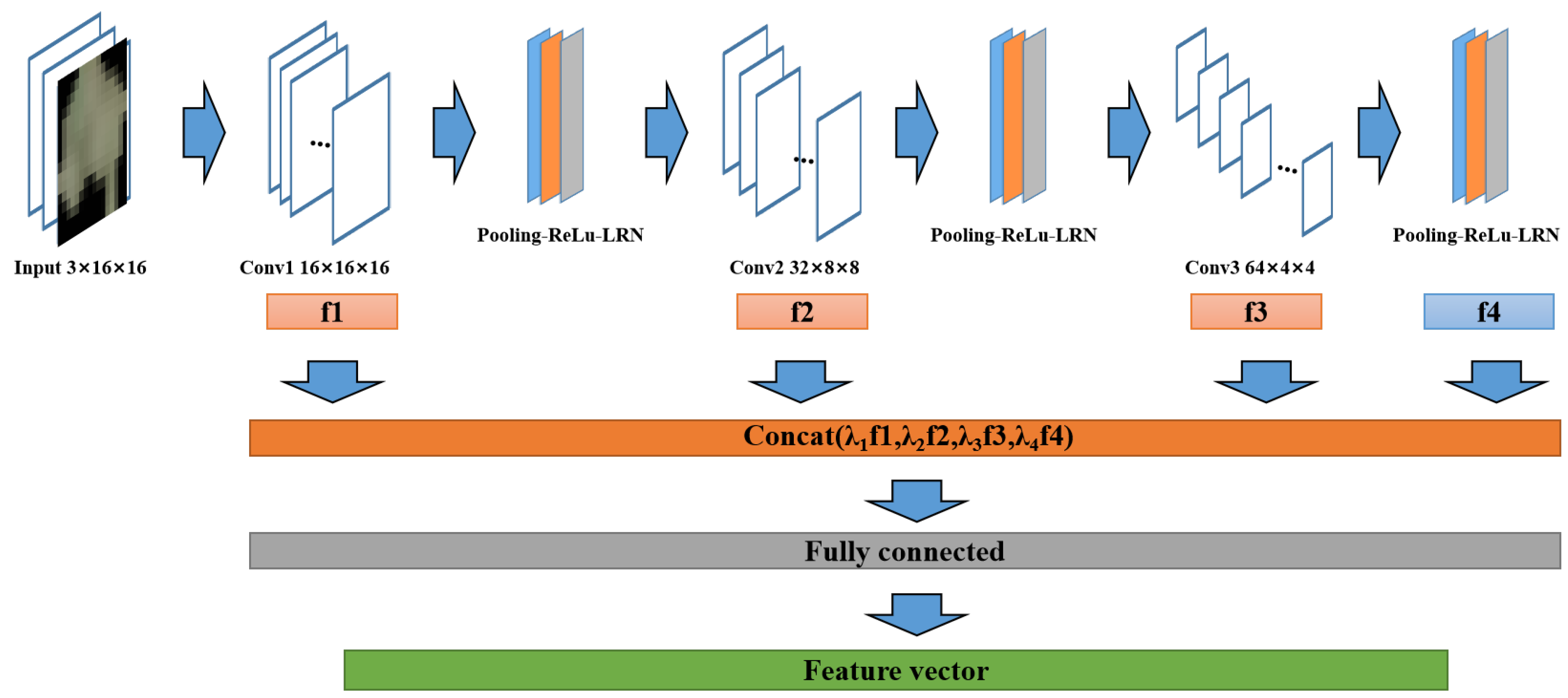
A feature extraction network at the super pixel level is constructed to extract the fast features of super pixels in cloud-containing remote sensing images at multi-scales. The cloud content in super pixels and the cloud-containing marker state information of adjacent super pixels are effectively utilized.
2.
A multi-view support vector machine cloud detection classifier based on fusion information is constructed and the solving algorithm based on quadratic convex optimization is given.
3.
We provide a multi-view classification dataset based on remote sensing cloud super pixels. The new model is used to classify the super pixels and synthesize the cloud mask bipartite graph. Experiments are carried out in images with different cloud contents to verify the effectiveness of the new method.
The rest of this article is organized as follows. Section 2 introduces the research status of multi-view learning and an advanced multi-view classification method. In Section 3, we introduce the framework of the proposed method in detail, including the multi-view feature extraction method and fusion information multi-view classification model. Section 4 shows the experimental results on two remote sensing datasets and discusses the results of the experiment. Finally, Section 5 summarizes the research work.

2. Related Work

2.1. Multi-View Learning

Multi-view learning algorithms can be divided into co-training, multi-kernel learning, and subspace learning [21,22]. The co-training algorithm iteratively maximizes mutual conventions on two distinct views to ensure consistency on the same validation data, such as multi-view collaborative clustering algorithm and research [23] using multiple collaborative training for document classification [24]. The multi-kernel learning (MKL) algorithm uses the kernels corresponding to different views and combines them linearly or nonlinearly to improve performance. For example, the support kernel machine (SKM) model introduced in [25], and the sequential minimum optimization (SMO) algorithm is developed to solve it. Multi-kernel framework with nonparallel support vector machine (MKNPSVM) works by integrating non-parallel support vector machines into the MKL framework to learn the optimal kernel combination [26]. The subspace learning algorithm assumes that the input view comes from a potential subspace and aims to realize the potential subspace shared by multiple views, such as SVM-2K combined with two support vector machines and kernel canonical correlation analysis (KCCA) [27], SVM classification method with coupling privileged kernel method [28], etc.

2.2. Coupling Privileged Kernel Method for Multi-View Learning

Tang et al. [28] proposed a simple and effective multi-view learning coupling privileged kernel method (MCPK). MCPK integrates consensus and complementarity principles into a unified framework. In particular, consistency is captured by coupling terms between two views. Because the multi-view data collected from different domains can complement each other, a different feature view can receive explicit privilege information from its view. MCPK can be built as Equation (1).
m i n w A , w B , ξ A , ξ B 1 2 ( w A 2 + γ w B 2 ) + C A i = 1 l ξ i A + C B i = 1 l ξ i B + C i = 1 l ξ i A ξ i B , s . t . y i ( w A · ϕ A ( x i A ) ) 1 ξ i A , y i ( w B · ϕ B ( x i B ) ) 1 ξ i B , ξ i A y i ( w B · ϕ B ( x i B ) ) , ξ i B y i ( w A · ϕ A ( x i A ) ) , ξ i A 0 , ξ i B 0 , i = 1 , , l .
where w A and w B are the weight vectors of view A and view B, respectively, and the two views are weighed by the non-negative trade-off parameter γ . As slack variables, ξ i A and ξ i A are constrained by the correction functions determined by the two views. The coupling term C i = 1 l ξ i A ξ i B makes the product of error variables of the two views as small as possible. When classifiers constructed from different views are more consistent, errors from both views are small, resulting in smaller couplings. Therefore, its consistency can be fully ensured. C is a non-negative coupling parameter that controls the influence of the coupling term. C A and C B are non-negative penalty parameters.

3. Proposed Method

3.1. Multi-View Feature Extraction

View A: Texture, boundary, and other features are extracted from the super pixel circumscribed rectangular region through a multi-layer joint convolutional neural network (CNN). Cloud area has similar shape to super pixel boundary, which is quite different from grassland area and water area boundary. In this paper, we use the inherent multi-scale pyramid level of a deep convolution network to develop a top architecture with horizontal connection, which is used to construct high-level feature maps at all scales. Features can be easily extracted by multi-scale feature extraction structure in the super pixel circumscribed rectangle, and texture, boundary, gradient, and other information can be obtained from multiple horizons. The feature extraction layer Conv3 in the deepest part will extract more abstract features. View A feature extraction is realized by cloud super pixel feature extraction network (CSPFE-Net); CSPFE-Net structure is shown in Figure 1. In the network structure, the super pixel external rectangular region has the input of 3 × 16 × 16 images. Conv refers to the convolution layer. Relu increases the nonlinear ability. Pooling downsampling is used to further extract the image. LRN is normalized to constrain the data within a certain range. Concat refers to stitching vectors. The features extracted from each feature extraction layer are weighted splicing, and are jointly output as the feature vector through the full connection layer. The feature vector with the super pixel output structure of 1 × 64 under the fine scale is sufficient to complete the feature representation.
View B: The color statistical characteristics extracted by the super pixel itself, excluding the black edge region of the circumscribed rectangle. Specifically, we calculate the mean, variance, maximum, minimum, and median of the data describing the color in each channel. S P i represents three-channel data for the i-th super pixel, and RGB color statistics can be calculated by Equation (3). The feature vector format of view b is 1 × 15 .
g e t C F ( x ) = [ m e a n ( x ) , s t d ( x ) , m a x ( x ) , m i n ( x ) , m e d i a n ( x ) ]
R G B f e a t u r e = [ g e t C F ( S P i ( R ) ) , g e t C F ( S P i ( G ) ) , g e t C F ( S P i ( B ) ) ]
where g e t C F ( x ) extracts and splices the statistical features of the data of one channel x; S P i ( R ) , S P i ( G ) , and S P i ( B ) represent three visible light channels: red, green, and blue.
View P: View P (privileged information view) is the feature of privileged information. The correction space guided by privilege information can correct the classification plane of multi-view, which can make the performance of multi-view classifier better. The feature of cloud-containing super pixel privileged information includes two parts. The first part is the specific cloud content in the super pixel. The second part is the label of the fast adjacent block of the super pixel. Generally, two super pixel blocks with the nearest center distance are selected, and this part is the feature vector of 1 × 3 .

3.2. Fusion Information Multi-View SVM Classification Method

Fusion information multi-view SVM classification method (FIMV-SVM) is based on MCPK, using feature extraction network and three-channel statistical features as view A and view B data, using privileged information view P to correct the separation hyperplane of view A and view B. The optimized structure constructed is as per Equation (4).
m i n w A , w B , w P , ξ A , ξ B , ξ P 1 2 ( w A 2 + γ w B 2 + γ P w P 2 ) + C A i = 1 l ξ i A + C B i = 1 l ξ i B + C P i = 1 l ξ i P + C i = 1 l ξ i A ξ i B , s . t . y i ( w A · ϕ A ( x i A ) ) 1 ξ i A , y i ( w B · ϕ B ( x i B ) ) 1 ξ i B , y i ( w P · ϕ P ( x i P ) ) 1 ξ i P , ξ i A y i ( w B · ϕ B ( x i B ) ) , ξ i B y i ( w A · ϕ A ( x i A ) ) , ξ i A y i ( w P · ϕ P ( x i P ) ) , ξ i B y i ( w P · ϕ P ( x i P ) ) , ξ i A 0 , ξ i B 0 , ξ i P 0 , i = 1 , , l .
In optimization problem Equation (4), w A 2 and w A 2 are regularization terms of view A and view B, w P 2 is a regularization term for privileged information view P, respectively. C A , C B , and C P are non-negative penalty parameters, ξ i A = [ ξ 1 A , , ξ l A ] , ξ i B = [ ξ 1 B , , ξ l B ] , and ξ i P = [ ξ 1 P , , ξ l P ] are non-negative slack parameters. γ is the balance parameter to balance the weight of view A and view B. γ P is used to weigh the influence of privileged information view P; ϕ A ( x i A ) , ϕ B ( x i B ) , and ϕ P ( x i P ) represent the mapping of views data. In the constraint, y i ( w P · ϕ P ( x i P ) ) 1 ξ i P denote that the slack variables are constrained by the view P, ξ i A y i ( w P · ϕ P ( x i P ) ) , and ξ i B y i ( w P · ϕ P ( x i P ) ) correcting constraints on the classification hyperplane through the correction hyperplane formed by privileged information. For the solution of the above optimization problem, it can be transformed into a Lagrangian dual problem and solved by solving quadratic convex optimization. The Lagrangian function is Equation (5).
L = 1 2 ( w A 2 + γ w B 2 + γ P w P 2 ) + C A i = 1 l ξ i A + C B i = 1 l ξ i B + C P i = 1 l ξ i P + C i = 1 l ξ i A ξ i B + i = 1 l α i A ( 1 ξ i A y i ( w A · ϕ i A ( x i A ) ) ) + i = 1 l α i B ( 1 ξ i B y i ( w B · ϕ i B ( x i B ) ) ) + i = 1 l α i P ( 1 ξ i P y i ( w P · ϕ i P ( x i P ) ) ) + i = 1 l λ i A ( y i ( w B · ϕ B ( x i B ) ) ξ i A ) + i = 1 l λ i B ( y i ( w A · ϕ A ( x i A ) ) ξ i B ) + i = 1 l μ i A ( y i ( w A · ϕ A ( x i A ) ) ξ i P ) + i = 1 l μ i B ( y i ( w B · ϕ B ( x i B ) ) ξ i P ) i = 1 l β i A ξ i A i = 1 l β i B ξ i B .
Therefore, the dual programming of Equation (4) can be obtained by finding the partial derivatives of the optimization parameters.
m i n 1 2 i = 1 l j = 1 l ( ( α i A λ i B ) y i K A ( x i A , x j A ) ( α j A λ j B ) y j + 1 γ ( α i B λ i A ) y i K B ( x i B , x j B ) ( α j B λ j A ) y j + 1 γ P ( α i P y i K P ( x i P , x j P ) α j P y j ) ) i = 1 l ( α i A + α i B + α i P ) + 1 C i = 1 l ( α i A + λ i A + μ i A + β i A C A ) ( α i B + λ i B + μ i B + β i B C B ) , s . t . α i A , α i B , λ i A , λ i B , μ i A , μ i B , β i A , β i B 0 .
where K A ( x i A , x j A ) , K B ( x i B , x j B ) , K P ( x i P , x j P ) represents the kernel mapping mode of view A, view B, and view P feature data, respectively. The optimization problem Equation (6) is a quadratic convex programming problem, which can be solved by the quadratic convex programming method. Solving the optimal parameters α i A , α i B , β i A , β i B , λ i A , λ i B , μ i A , μ i B , we use the Karush–Kuhn–Tucker(KKT) [29] condition to obtain the optimal result w A and w B . The calculation results are shown in Equations (7) and (8).
w A = i = 1 l ( α i A y i λ i B y i ) ϕ A ( x i A ) ,
w B = i = 1 l ( α i B y i λ i A y i ) ϕ B ( x i B ) .
After obtaining the optimal w A and w B , we use the following formula to predict the labels of the new samples ( x A , x B ) from view A and view B. The final predictor of multi-views can be constructed as the average prediction factor of each view and is shown in (9).
f = s i g n ( 1 2 f A ( x A ) + 1 2 f B ( x B ) ) = s i g n ( 1 2 w A ϕ A ( x A ) + 1 2 w B ϕ B ( x B ) ) .
where f A represents the decision function of view A and f B represents the decision function of view B. The FIMV-SVM solution process is clearly represented in Algorithm 1.

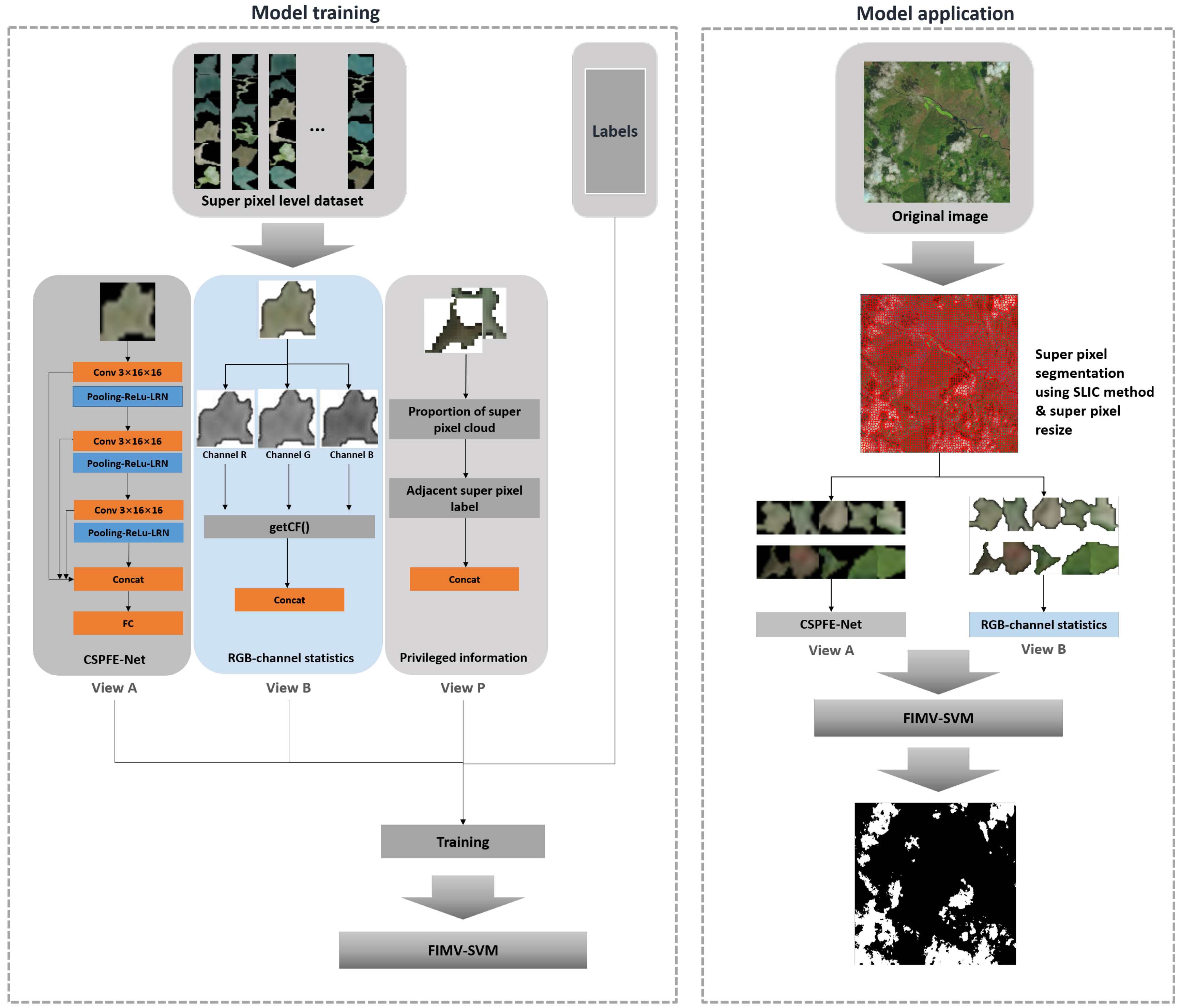
3.3. Cloud Detection Model Training and Application Process

Combined with the above contents, the cloud detection model method can be summarized. The specific process is shown in Figure 2. Notably, privileged information does not appear in the application phase.
Algorithm 1 QP Algorithm for FIMV-SVM
Require: S = x i A , x i B , x i P , y i y = 1 l = x i A ; 1 , x i B ; 1 , ( x i P , 1 ) i = 1 l , y i { + 1 , 1 }
Ensure: Decision functions: f = s i g n ( 1 2 w A ϕ A ( x A ) + 1 2 w B ϕ B ( x B ) )
1:
Grid method generates parameter sets: p a r a S e t = C A , C B , C P , C , γ , γ P i = 1 n .
2:
for each i [ 1 , n ] do
3:
   Set parameters C A , C B , C P , C , γ , γ P = p a r a S e t [ i , : ] .
4:
   Set kernels function of view A, view B and view P: K A ( x i A , x j A ) , K B ( x i B , x j B ) , K P ( x i P , x j P ) .
5:
   Create and solve quadratic programming problem and Solving quadratic programming and retaining optimal parameters α i A , α i B , β i A , β i B , λ i A , λ i B , μ i A , μ i B .
6:
   Get the optimal weight w A and w B by substituting formula:
w A = i = 1 l ( α i A y i λ i B y i ) ϕ A ( x i A ) , w B = i = 1 l ( α i B y i λ i A y i ) ϕ B ( x i B ) .
7:
   Decision function is solved by parameters w A and w B .
8:
   The accuracy of statistical validation set was calculated as A C C [ i ] , W A [ i ] = w A , W B [ i ] = w B .
9:
end for
10:
The final w A , w B :
w A = W A [ f i n d ( a c c = = m a x ( A C C ) ) ] , w B = W B [ f i n d ( a c c = = m a x ( A C C ) ) ] .
In the model training phase, the following steps are taken: (1) The super pixels come from simple linear iterative cluster (SLIC) method [30], which is used for super pixel division in the original image dataset to construct the dataset with super pixel blocks as the classification objects; (2) three different feature extraction methods are used to extract the feature of super pixels one by one, and the feature vectors of view A, view B, and view P are composed; (3) FIMV-SVM classifier is trained by using the extracted numerical feature dataset and labels.
In the model application phase, the following steps are taken: (1) The image to be processed is divided by SLIC super pixel segmentation method, and then the super pixel block is resized; (2) the features of view A and view B are extracted from the super pixel set one by one to form their feature vectors; (3) super pixel classification object view A, view B, two view feature vectors, are input through the FIMV-SVM decision function to obtain the corresponding classification results; (4) the final segmentation cloud mask result is formed by combining the super pixel classification results.

4. Experiment

Our experiment was carried out on a personal computer with i7-6500 CPU and 16 GB RAM. The environment used in the experiment is Python 3.7 combined with pyTorch framework (version 1.11.0), and the cvxopt tool [31] on MATLAB 2016b is used to solve the convex optimization problem.
For the experiment in GF-1_WHU remote sensing images [32] and datasets of Cloud-38 [33], the detailed description is shown in Table 1. The original high-pixel image is divided into sub-images of 400 × 400 × 3 , and only their visible light channels are used.
In the process of setting the level of segmentation parameters of super pixel segmentation, considering that the super pixel object needs to have certain information inclusion ability, in the image of 400 × 400 × 3 , the classification levels are 1000, 1600, 2000, 2400, and 3000, which can be divided into about 160, 100, 80, 67, and 54 pixels in the super pixel block. In order to explore the optimal parameters of the super pixel partition level, we construct a parameter optimization dataset from the original datasets with the size of 1000. A total of 80% of the parameter optimization dataset is used for training, and the rest is used for testing. The average accuracy in the test process is used as the evaluation index. The experimental results are shown in Figure 3. The optimal result is obtained when the super pixel level is 2000, which shows that the number of super pixels in the super pixel is about 80, which is suitable for the smallest unit of the cloud recognition task. Therefore, for the super pixel segmentation method using convenient and efficient SLIC method, the segmentation level is 2000, that is, an image contains about 2000 super pixels, and each super pixel contains about 80 pixels. By resize operation, the number of rectangular pixels is about 256 pixels ( 16 × 16 ) . The resize process uses the imresize function of MATLAB software, and imresize uses bicubic interpolation by default. The super pixel blocks with cloud content exceeding 45% are automatically labeled as cloud super pixels, and the others are labeled as non-cloud super pixels.

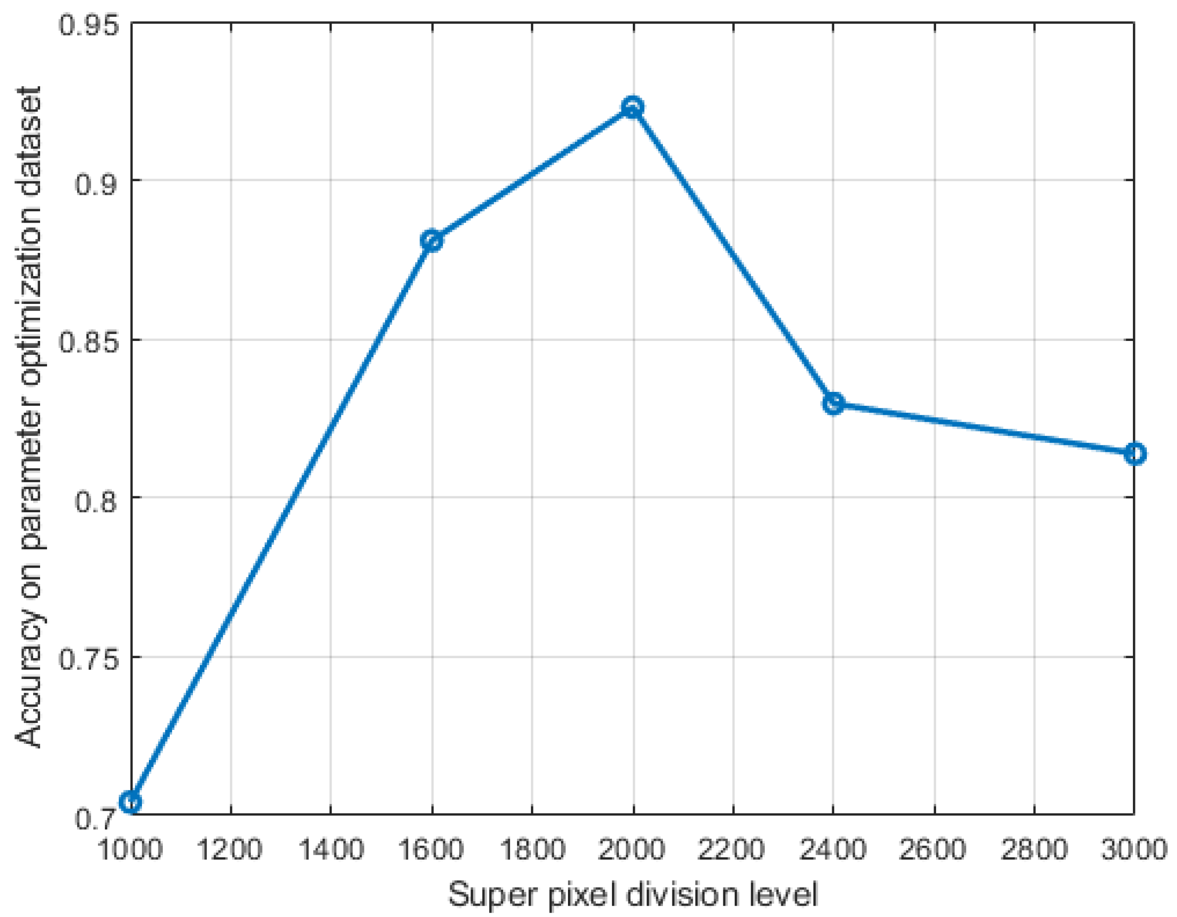
4.1. Parameter Setting

In the experiment, we set the following parameters. The values of λ 1 , λ 2 , λ 3 , and λ 4 in CSPFE-Net of view A are 0.3, 0.3, 0.2, and 0.2. FIMV-SVM parameters are determined by grid search method and five-fold cross validation during training. The determination of parameters is based on the highest accuracy. C, C A , C B , and C P select their values from the set [ 10 3 , 10 2 , 10 1 , 1 , 10 , 10 2 , 10 3 ] . The value set of γ and γ P is [ 0.2 , 0.4 , 0.6 , 0.8 , 1 ] . Gaussian radial basis function (RBF) kernel function K ( x i , x j ) = e x p ( x i x j 2 2 σ ) is the kernel function of SVM method, σ for the Gaussian RBF kernel function is selected from [ 10 3 , 10 2 , 10 1 , 1 , 10 , 10 2 , 10 3 ] . For the association between parameter tuning and training, see Algorithm 1 above.

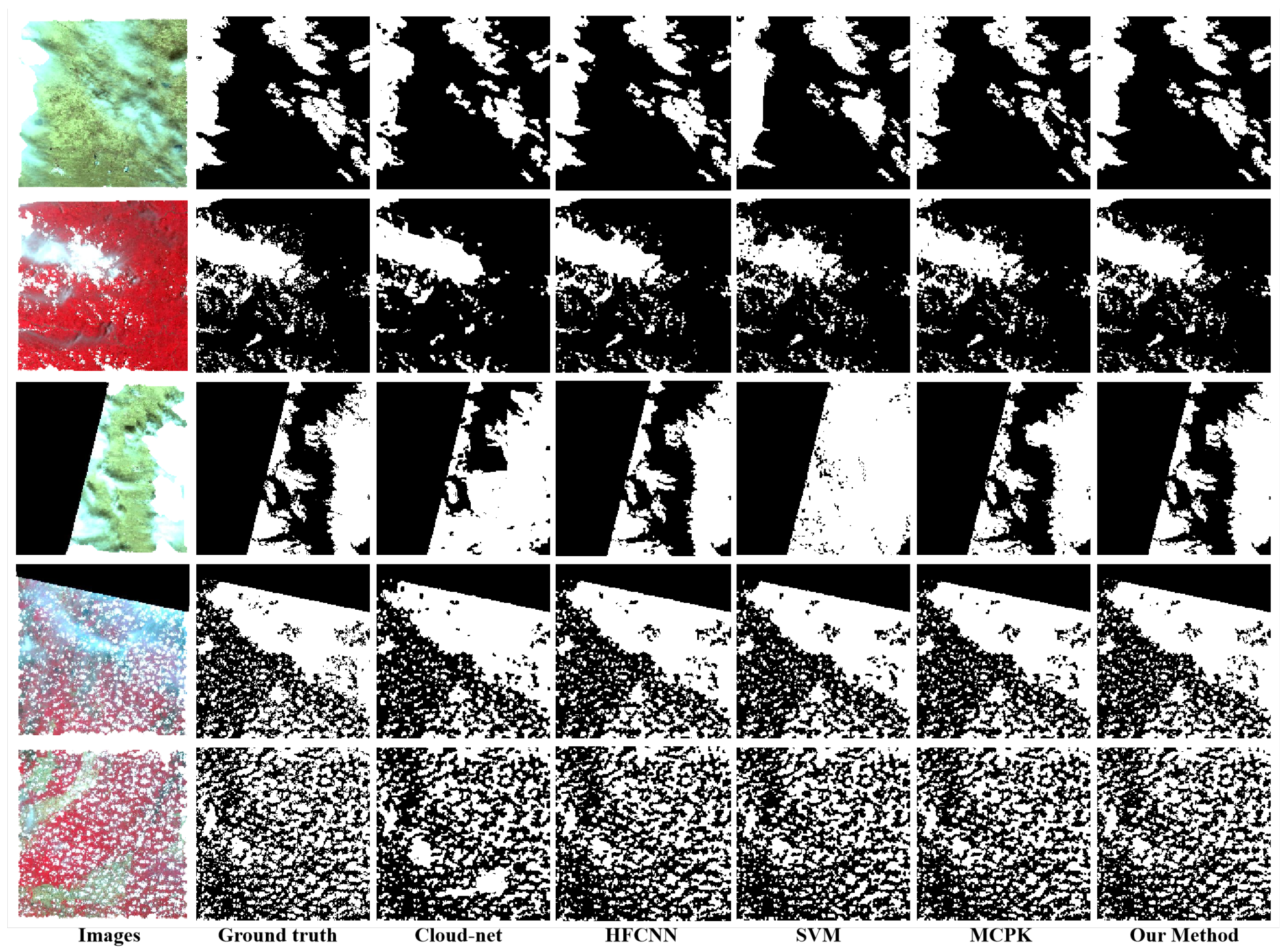
4.2. Visual Performance

We compare the proposed method with several advanced cloud detection methods. Cloud-Net is a cloud detection method based on deep learning and is widely used as the baseline of cloud detection experiments. Hierarchical fusion convolutional neural network (HFCNN) [19] is a network detection method with multi-level feature extraction, and HFCNN is a super-pixel-level judgment method. Furthermore, we added the SVM method and the MCPK method. In the SVM method, the extracted view A data and view B data are used as one-dimensional features for training. In MCPK, the data of view A and view B are used. Through these two experiments, we can explore the effectiveness of multi-view learning and privileged information addition.
Typical cloud-containing image blocks are selected from GF-1_WHU and Cloud-38 to display the detection results. These images have a variety of cloud coverage and backgrounds. The comparison results with the proposed method are shown in Figure 4 and Figure 5. In the figures, from left to right, are original image, ground truth, Cloud-net, HFCNN, SVM, MCPK, and our method. From the visual results, on the whole, the proposed method is closer to ground truth. There are several aspects worth noting. In Figure 4, the test object in the third line is an image with highlighted features. Cloud-Net has a certain misjudgment, and SVM method judges a large area into a cloud. Compared with HFCNN, the proposed method is more rigorous for thin cloud detection. SVM methods often lack large-scale cloud areas, and MCPK will misjudge to a certain extent in continuous clouds.

4.3. Quantitative Analysis

In the description of the overall results, the Jaccard index is used to describe the similarity between the predicted mask and the real mask, which is widely used in the performance evaluation of cloud detection tasks. Precision is the ratio that predicts the number of true values to the number of cloud tags in cloud data. Recall represents how many clouds can be predicted in all marked cloud data. Specificity index is used to measure the integrity of error prediction, and the overall accuracy index is used to represent the accuracy of the cloud/non-cloud binary classification. F1-score considers the relationship between precision and recall. The calculation method of each evaluation index is shown as Equations (10)–(15).
We divide each data image in GF-1_WHU and Cloud-38 into 400 × 400 × 3 specifications, and randomly select 80% of the dataset as the training set image, which is the test set image. Specifically, in the GF-1_WHU dataset, there are 4246 images, including 3369 training images and 850 test images. In the cloud-38 dataset, there are 15,200 images, including 12,160 training images and 3040 test images. Each index data is shown as (mean ± variance).
J a c c a r d I n d e x = T P T P + F N + F P
P r e c i s i o n = T P T P + F P
R e c a l l = T P T P + F N
S p e c i f i c t i t y = T N T N + F P
O v e r a l l A c c u r a c y = T P + T N T P + T N + F P + F N
F 1 S c o r e = 2 × P r e c i s i o n × R e c a l l P r e c i s i o n + R e c a l l
where T P represents the number of positive samples with positive judgment results, T N represents the number of negative samples with negative judgment results, F P represents the number of negative samples with positive judgment results, and F N represents the number of positive samples with negative judgment results.
As shown in Table 2 and Table 3, our method achieves high scores in both groups of test results. The Cloud-net [15] method needs a certain number of training sets to annotate data, and cannot use the location information of pixel blocks. HFCNN also uses super pixels as the basic unit of cloud detection, but it uses only one feature extraction method, and cannot use the privilege information marked by super pixels, so it performs poorly in some confusing areas. The basis of its use is 32 × 32 × 3 and the segmentation effect may be rougher. By comparing the SVM, MCPK, and our methods, it is proved that the multi-view structure has better performance than the method of directly stitching combined features. At the same time, thanks to the feature extraction of super pixel multi-view and the utilization of privilege information, our method is more accurate for the recognition of the cloud area. The experimental results show that no matter whether the type of substrate in the background is more or less, our method can obtain excellent results, and the results of each index prove the feasibility and effectiveness of the proposed remote cloud sensing detection method.

5. Conclusions

This paper mainly studies the three-channel remote sensing cloud detection method based on the fusion of multi-view information at the super pixel level. Firstly, the segmented super pixels are used to establish a super pixel remote sensing image database. Secondly, a variety of feature extraction mechanisms are used to extract three view features of super pixel blocks containing privileged information views. Finally, an SVM classifier that can utilize privileged information features is constructed, and a solution strategy based on quadratic convex optimization is proposed. The classifier is used to judge the super pixel category organization one by one to generate the cloud mask. Experiments are carried out on GF1_WHU and Cloud-38 datasets with different cloud content data. From the results of qualitative and quantitative analysis, we can see that the proposed method has good performance, and it also has good detection effect in scenarios with large differences in cloud distribution and cloud content. In the future, we consider improving the model by using transfer learning technology to make the model quickly adapt to the cloud recognition of multi-style remote sensing images. The algorithm proposed in this paper is based on the improvement of SVM binary classifiers. It is necessary to study a new strategy for multi-classification tasks such as accurate cloud classification, which is also a direction worthy of study in the future.

Author Contributions

Conceptualization, Q.H. and Y.X.; methodology, Q.H. and W.Z.; software, Q.H.; validation, Q.H., Y.X. and W.Z.; writing—original draft preparation, Q.H.; writing—review and editing, Q.H., Y.X. and W.Z.; visualization, Q.H.; supervision, Y.X.; project administration, W.Z. All authors have read and agreed to the published version of the manuscript.

Funding

This research was funded by Tianjin “Project + Team” Key Training Project grant number XC202022 and Tianjin Research Innovation Project for Postgraduate Students grant number 2021YJSS095.

Institutional Review Board Statement

Not applicable.

Informed Consent Statement

Not applicable.

Data Availability Statement

Not applicable.

Conflicts of Interest

The authors declare no conflict of interest.

Abbreviations

The following is a description of the abbreviations used in this paper.
SVMSupport vector machine
MKLMulti-kernel learning
SMOSequential minimum optimization
MKNPSVMMulti-kernel framework with nonparallel support vector machine
KCCAKernel canonical correlation analysis
FCNFull convolution networks
MCPKMulti-view learning coupling privileged kernel method
CNNConvolutional neural network
CSPFE-NetCloud super pixel feature extraction network
FIMV-SVMFusion information multi-view SVM
KKTKarush–Kuhn–Tucke
SLICSimple linear iterative cluster
HFCNNHierarchical fusion convolutional neural network
RBFRadial basis function

References

  1. Sola, I.; Álvarez-Mozos, J.; González-Audícana, M. Inter-Comparison of Atmospheric Correction Methods on Sentinel-2 Images Applied to Croplands. In Proceedings of the 2018 IEEE International Geoscience and Remote Sensing Symposium, IGARSS 2018, Valencia, Spain, 22–27 July 2018; IEEE: Piscataway Township, NJ, USA, 2018; pp. 5940–5943. [Google Scholar]
  2. Vermote, E.F.; Saleous, N.; Justice, C.O. Atmospheric correction of MODIS data in the visible to middle infrared: First results. Remote Sens. Environ. 2002, 83, 97–111. [Google Scholar] [CrossRef]
  3. Irish, R.R.; Barker, J.L.; Goward, S.N.; Arvidson, T. Characterization of the Landsat-7 ETM+ automated cloud-cover assessment (ACCA) algorithm. Photogramm. Eng. Remote Sens. 2006, 72, 1179–1188. [Google Scholar] [CrossRef] [Green Version]
  4. Zhu, Z.; Woodcock, C.E. Object-based cloud and cloud shadow detection in Landsat imagery. Remote Sens. Environ. 2012, 118, 83–94. [Google Scholar] [CrossRef]
  5. Bley, S.; Deneke, H. A threshold-based cloud mask for the high-resolution visible channel of Meteosat Second Generation SEVIRI. Atmos. Meas. Tech. 2013, 6, 2713–2723. [Google Scholar] [CrossRef] [Green Version]
  6. Jedlovec, G.J.; Haines, S.L.; LaFontaine, F.J. Spatial and temporal varying thresholds for cloud detection in GOES imagery. IEEE Trans. Geosci. Remote Sens. 2008, 46, 1705–1717. [Google Scholar] [CrossRef]
  7. Zhang, Q.; Xiao, C. Cloud detection of RGB color aerial photographs by progressive refinement scheme. IEEE Trans. Geosci. Remote Sens. 2014, 52, 7264–7275. [Google Scholar] [CrossRef] [Green Version]
  8. Li, P.; Dong, L.; Xiao, H.; Xu, M. A cloud image detection method based on SVM vector machine. Neurocomputing 2015, 169, 34–42. [Google Scholar] [CrossRef]
  9. Le Hégarat-Mascle, S.; André, C. Use of Markov random fields for automatic cloud/shadow detection on high resolution optical images. ISPRS J. Photogramm. Remote Sens. 2009, 64, 351–366. [Google Scholar] [CrossRef]
  10. Shao, Z.; Deng, J.; Wang, L.; Fan, Y.; Sumari, N.S.; Cheng, Q. Fuzzy autoencode based cloud detection for remote sensing imagery. Remote Sens. 2017, 9, 311. [Google Scholar] [CrossRef] [Green Version]
  11. Ishida, H.; Oishi, Y.; Morita, K.; Moriwaki, K.; Nakajima, T.Y. Development of a support vector machine based cloud detection method for MODIS with the adjustability to various conditions. Remote Sens. Environ. 2018, 205, 390–407. [Google Scholar] [CrossRef]
  12. Yuan, Y.; Hu, X. Bag-of-words and object-based classification for cloud extraction from satellite imagery. IEEE J. Sel. Top. Appl. Earth Obs. Remote Sens. 2015, 8, 4197–4205. [Google Scholar] [CrossRef]
  13. Mohajerani, S.; Krammer, T.A.; Saeedi, P. Cloud detection algorithm for remote sensing images using fully convolutional neural networks. arXiv 2018, arXiv:1810.05782. [Google Scholar]
  14. Manzo, M.; Pellino, S. Voting in transfer learning system for ground-based cloud classification. Mach. Learn. Knowl. Extr. 2021, 3, 28. [Google Scholar] [CrossRef]
  15. Mohajerani, S.; Saeedi, P. Cloud-Net: An end-to-end cloud detection algorithm for Landsat 8 imagery. In Proceedings of the IGARSS 2019—2019 IEEE International Geoscience and Remote Sensing Symposium, Yokohama, Japan, 28 July–2 August 2019; IEEE: Piscataway Township, NJ, USA,, 2019; pp. 1029–1032. [Google Scholar]
  16. Yan, Z.; Yan, M.; Sun, H.; Fu, K.; Hong, J.; Sun, J.; Zhang, Y.; Sun, X. Cloud and cloud shadow detection using multilevel feature fused segmentation network. IEEE Geosci. Remote Sens. Lett. 2018, 15, 1600–1604. [Google Scholar] [CrossRef]
  17. Tan, K.; Zhang, Y.; Tong, X. Cloud extraction from Chinese high resolution satellite imagery by probabilistic latent semantic analysis and object-based machine learning. Remote Sens. 2016, 8, 963. [Google Scholar] [CrossRef] [Green Version]
  18. Xie, F.; Shi, M.; Shi, Z.; Yin, J.; Zhao, D. Multilevel cloud detection in remote sensing images based on deep learning. IEEE J. Sel. Top. Appl. Earth Obs. Remote Sens. 2017, 10, 3631–3640. [Google Scholar] [CrossRef]
  19. Liu, H.; Du, H.; Zeng, D.; Tian, Q. Cloud detection using super pixel classification and semantic segmentation. J. Comput. Sci. Technol. 2019, 34, 622–633. [Google Scholar] [CrossRef]
  20. Gao, X.; Fan, L.; Xu, H. Multiple rank multi-linear kernel support vector machine for matrix data classification. Int. J. Mach. Learn. Cybern. 2018, 9, 251–261. [Google Scholar] [CrossRef]
  21. Xu, C.; Tao, D.; Xu, C. A survey on multi-view learning. arXiv 2013, arXiv:1304.5634. [Google Scholar]
  22. Tang, J.; He, Y.; Tian, Y.; Liu, D.; Kou, G.; Alsaadi, F.E. Coupling loss and self-used privileged information guided multi-view transfer learning. Inf. Sci. 2021, 551, 245–269. [Google Scholar] [CrossRef]
  23. Appice, A.; Malerba, D. A co-training strategy for multiple view clustering in process mining. IEEE Trans. Serv. Comput. 2015, 9, 832–845. [Google Scholar] [CrossRef]
  24. Kim, D.; Seo, D.; Cho, S.; Kang, P. Multi-co-training for document classification using various document representations: TF–IDF, LDA, and Doc2Vec. Inf. Sci. 2019, 477, 15–29. [Google Scholar] [CrossRef]
  25. Cao, L.-L.; Huang, W.B.; Sun, F.-C. Optimization-based extreme learning machine with multi-kernel learning approach for classification. In Proceedings of the 2014 22nd International Conference on Pattern Recognition, Stockholm, Sweden, 24–28 August 2014; IEEE: Piscataway Township, NJ, USA, 2014; pp. 3564–3569. [Google Scholar]
  26. Tang, J.; Tian, Y. A multi-kernel framework with nonparallel support vector machine. Neurocomputing 2017, 266, 226–238. [Google Scholar] [CrossRef]
  27. Chao, G.; Sun, S. Consensus and complementarity based maximum entropy discrimination for multi-view classification. Inf. Sci. 2016, 367, 296–310. [Google Scholar] [CrossRef]
  28. Tang, J.; Tian, Y.; Liu, D.; Kou, G. Coupling privileged kernel method for multi-view learning. Inf. Sci. 2019, 481, 110–127. [Google Scholar] [CrossRef]
  29. Deng, N.; Tian, Y.; Zhang, C. Support Vector Machines: Optimization Based Theory, Algorithms, and Extensions; CRC Press: Boca Raton, FL, USA, 2012. [Google Scholar]
  30. Achanta, R.; Shaji, A.; Smith, K.; Lucchi, A.; Fua, P.; Süsstrunk, S. SLIC super pixels compared to state-of-the-art super pixel methods. IEEE Trans. Pattern Anal. Mach. Intell. 2012, 34, 2274–2282. [Google Scholar] [CrossRef] [Green Version]
  31. Grant, M.; Boyd, S.; Ye, Y. CVX: Matlab Software for Disciplined Convex Programming. 2008. Available online: http://cvxr.com/cvx/ (accessed on 15 July 2022).
  32. Li, Z.; Shen, H.; Li, H.; Xia, G.; Gamba, P.; Zhang, L. Multi-feature combined cloud and cloud shadow detection in GaoFen-1 wide field of view imagery. Remote Sens. Environ. 2017, 191, 342–358. [Google Scholar] [CrossRef] [Green Version]
  33. Roy, D.P.; Wulder, M.A.; Loveland, T.R.; Woodcock, C.E.; Allen, R.G.; Anderson, M.C.; Helder, D.; Irons, J.R.; Johnson, D.M.; Kennedy, R.; et al. Landsat-8: Science and product vision for terrestrial global change research. Remote Sens. Environ. 2014, 145, 154–172. [Google Scholar] [CrossRef] [Green Version]
Figure 1. CSPFE-NET structure.
Applsci 12 07295 g001
Figure 2. FIMV-SVM cloud detection model training and application process framework.
Applsci 12 07295 g002
Figure 3. Performance of different super pixel classification levels on parameter optimization dataset.
Applsci 12 07295 g003
Figure 4. The performance of several methods on GF-1_WHU dataset [32] with different cloud distribution styles.
Applsci 12 07295 g004
Figure 5. The performance of several methods on Cloud-38 dataset [33] with different cloud distribution styles.
Applsci 12 07295 g005
Table 1. Public dataset description.
NameNumber of ImgagesResource AcquisitionRemarks
GF-1_WHU108http://sendimage.whu.edu.cn/en/mfc-validation-data/ (accessed on 15 July 2022)GF-1_WHU includes 108 GF-1 wide field of view (WFV) level-2A scenes and its reference cloud and cloud shadow masks.
Cloud-3838https://www.kaggle.com/datasets/sorour/38cloud-cloud-segmentation-in-satellite-images/download (accessed on 15 July 2022)There are four spectral channels, namely, red (band 4), green (band 3), blue (band 2), and near-infrared (band 5).
Table 2. Performance on GF-1_WHU test dataset (mean ± variance (%)).
MethodJaccard IndexPressionRecallSpecificityOverall AccuracyF1-Score
Cloud-Net [15]81.93 ± 7.2287.03 ± 5.4893.49 ± 4.3682.86 ± 4.3488.46 ± 3.6891.21 ± 4.46
HFCNN [19]87.94 ± 5.1291.87 ± 4.0596.02 ± 5.1391.28 ± 3.7492.79 ± 5.0494.36 ± 4.76
SVM67.12 ± 3.7771.36 ± 5.1492.13 ± 5.4972.56 ± 4.8778.85 ± 3.2479.62 ± 3.64
MCPK85.32 ± 4.1987.93 ± 5.3396.07 ± 3.9685.77 ± 5.0890.76 ± 4.3992.43 ± 3.13
Our method91.69 ± 1.3494.67 ± 2.0197.38 ± 1.6593.04 ± 2.1296.31 ± 1.4696.03 ± 1.72
Table 3. Performance on Cloud-38 test dataset (mean ± variance (%)).
MethodJaccard IndexPressionRecallSpecificityOverall AccuracyF1-Score
Cloud-Net [15]87.13 ± 5.1491.22 ± 4.3795.94 ± 3.8989.03 ± 4.3493.14 ± 5.3692.87 ± 4.68
HFCNN [19]92.04 ± 3.6992.95 ± 3.9898.25 ± 5.0192.24 ± 4.3695.86 ± 5.2394.21 ± 3.67
SVM79.02 ± 4.3782.83 ± 5.0492.87 ± 4.7682.78 ± 3.8586.74 ± 4.1987.86 ± 3.92
MCPK87.45 ± 3.9492.32 ± 4.1896.83 ± 5.0388.34 ± 4.7692.89 ± 5.1494.03 ± 3.87
Our method94.87 ± 1.2495.28 ± 1.3998.74 ± 2.0793.48 ± 2.1197.28 ± 1.4797.37 ± 1.86
Publisher’s Note: MDPI stays neutral with regard to jurisdictional claims in published maps and institutional affiliations.

