Abstract
This work is devoted to the analysis of the background seismic noise acquired at the volcanoes (Campi Flegrei caldera, Ischia island, and Vesuvius) belonging to the Neapolitan volcanic district (Italy), and at the Colima volcano (Mexico). Continuous seismic acquisition is a complex mixture of volcanic transients and persistent volcanic and/or hydrothermal tremor, anthropogenic/ambient noise, oceanic loading, and meteo-marine contributions. The analysis of the background noise in a stationary volcanic phase could facilitate the identification of relevant waveforms often masked by microseisms and ambient noise. To address this issue, our approach proposes a machine learning (ML) modeling to recognize the “fingerprint” of a specific volcano by analyzing the background seismic noise from the continuous seismic acquisition. Specifically, two ML models, namely multi-layer perceptrons and convolutional neural network were trained to recognize one volcano from another based on the acquisition noise. Experimental results demonstrate the effectiveness of the two models in recognizing the noisy background signal, with promising performance in terms of accuracy, precision, recall, and F1 score. These results suggest that persistent volcanic signals share the same source information, as well as transient events, revealing a common generation mechanism but in different regimes. Moreover, assessing the dynamic state of a volcano through its background noise and promptly identifying any anomalies, which may indicate a change in its dynamics, can be a practical tool for real-time monitoring.
1. Introduction
Seismic noise consists of persistent vibrations of the ground generated by a variety of sources: oceanic loading, atmospheric phenomena, and human and environmental activities [1]. Meteo-marine microseism, caused by wind or ocean waves, is particularly energetic near the coast [2,3,4]. This microseism, related to the interaction between ocean and crust, is generally characterized by frequencies below 1 Hz [5]. The phenomenon is well-documented in the literature [6]: for example, in the Gulf of Pozzuoli (Italy), it is mainly concentrated in the band 0.1–0.5 Hz and its amplitude depends on the sea/weather condition [4,7,8,9]. In cities, seismic noise, also known as ambient or cultural noise, is due to several processes, such as traffic, flights, trains, industries, etc. [2]. It is generally characterized by shallow propagation and spectral content in the frequency band 1–10 Hz. Another important characteristic is that it shows some specific periodicities: daily changes (night/day alternation) and weekly variation (working days vs. weekends), with a lowering level during holidays (see, e.g., [5]).
Due to the persistent nature of seismic noise, continuous recordings acquired by seismometers are affected by this background, which can mask signals such as earthquakes; thus, a general task in Earth science is the extraction of buried relevant waveforms (see, e.g., [10,11]). The problem is particularly complex in volcanic environments because of the presence of both transient and sustained signals generated by different sources that have a pure volcanic origin or are related to external forcing. Much interest is generally devoted to transients, such as volcano-tectonic earthquakes (VT), long-period (LP) and very-long-period (VLP) events, and explosion quakes, but significant information on the volcanic source is also provided by the investigation of persistent signals such as volcanic and/or hydrothermal tremor. However, both volcanic transients and persistent tremors are very often masked by microseisms and ambient noise, especially when recorded in densely populated areas [2,12].
The interest in volcanic or hydrothermal tremor comes from the evidence that it represents the seismic signature of magmatic and/or hydrothermal fluids flowing through volcanic structures [13]. Its detection becomes difficult when it is overcome by continuous explosion quakes [14] or by LP swarms, as in the cases of the Deception (Antarctica), Arenal (Costa Rica), and Campi Flegrei (Italy) volcanoes [15,16,17]. Often, tremor shares common features with explosion quakes or LP events in both the time and frequency domains, revealing a common mechanism that could explain their generation [15]. The tremor source location can provide indications on the fluid movement, but it is very difficult because of the absence of a clear onset [13], which does not allow the application of standard techniques based on the arrival picking. Tremors are located superficially (<5 km) and observed in several structures such as eruptive craters and conduits [18], gas slug bursts at surface vents [14,19,20], lava lakes [21,22], lava flows [23], shallow dikes [24], and magma–water aquifer interfaces, or due to the coupling between hydrothermal fluid-flow and solid structures [15,25].
Besides the adoption of well-consolidated methodologies based on the seismological analysis of the waveforms [26,27,28], the characterization of typical events occurring on volcanoes, in these last years, has been also performed by using the recent machine learning (ML) techniques, such as artificial neural networks (ANN), multi-layer perceptrons (MLP) [29,30], convolutional neural networks (CNN) [31], etc. For a review, please consider [32]. These techniques have been applied to obtain detection and classification of transient signals both of tectonic and volcanic origin, such as VT earthquakes, LP events, explosion quakes, etc., from background noise. In this context, a very recent application has regarded the detection of source events at the Colima and Vesuvius volcanoes, whose classification is the basis for the construction of a suitable ontology in which the events are semantically annotated. This framework can be embedded in early warning systems to ensure an effective monitoring of dangerous volcanoes and improve the time and accuracy of hazard forecasts [33,34]. In a few cases, ML approaches have been applied to identify episodic volcanic tremors [30] and (even less) to nonstationary seismic noise of natural and/or artificial origin, usually affecting continuous waveforms [35].
This work proposes a machine learning solution, inspired by [34], for analyzing the background seismic signal acquired in different volcanic areas. To the best of our knowledge, this is the first attempt in the seismological field in which the proposed approach successfully identifies the source that generates it. The ML-based classification of background seismic signal, as a hallmark for recognition of the generating volcanic source, is thus the main contribution of the present research.
Specifically, we will study four volcanoes: Campi Flegrei, Ischia, and Vesuvius (Italy), and Colima (Mexico), each one characterized by peculiar patterns of seismic activity. The main aim is to show that the MLP and CNN methods are able to classify the background seismic signal, even containing different contributions (microseism, cultural noise, and volcanic/hydrothermal tremor). The classified signal can be considered as a kind of fingerprint, which allows the identification of a volcano, among others. The proposed approach, when applied to continuous seismic acquisitions, can promptly reveal anomalies or variations of the background motion, thus providing information about changes in the source process much earlier than the occurrence of potentially dangerous events such as volcanic eruptions.
2. Materials and Methods
2.1. Seismological Overview
Our study area comprises both hydrothermal systems (such as Campi Flegrei and Ischia) and stratovolcanoes such as Vesuvius and Colima.
Campi Flegrei and Ischia belong to the Phlegrean Volcanic District, southern Italy. In both cases, besides transient phenomena, the background signal is characterized by the presence of a persistent hydrothermal tremor, meteo-marine contribution, and anthropogenic noise [36,37]. The origin of the tremor can be ascribed to the vibrations of the shallow hydrothermal system caused by the fluid motion. Many examples of this mechanism have been found everywhere, each characterized by specific periodicities, from Old Faithful Geyser, Yellowstone (USA) [38] to the Nisyros caldera (Greece), where researchers found oscillations on the order of 40–60 min related to gas instability [39]. Vesuvius is in a quiescent state whose dynamics is constantly monitored to detect eventual variations and/or precursors of eruption [7]. Colima, instead, is in an unrest phase, displaying a variety of eruption styles, from phreatic explosions and major block-lava extrusions, up to large explosive events [27].
The background seismic acquisition at Campi Flegrei is a complex mixture of hydrothermal tremor, meteo-marine microseism, anthropogenic noise, VT swarms and occasionally LP events, and regional earthquakes [9]. Some of these elements can also share the same frequency content, making the discrimination even more difficult. This is the case for the band lower than 1 Hz, in which we find the signature of both meteo-marine microseism and hydrothermal components [36] at specific frequencies of 0.3 Hz and 0.8 Hz, respectively. Instead, anthropogenic noise mainly affects the band above 1 Hz, specifically 4–5 Hz and 10–12 Hz, and it is characterized by the day/night alternation in the amplitude level [40]. The sustained hydrothermal tremor, mainly peaked at 1 Hz, is generated by the shallow geothermal aquifer nearby the Solfatara crater [36,41]. Here, there is a consistent flux of hot fluids mixed with meteoric water coming from the boiling mud pools and the Pisciarelli fumaroles [42,43]. Moreover, LP events appear to be the enhancement of the hydrothermal tremor under suitable conditions, sharing the same polarization patterns [15,44]; they are associated with the vibrations of the shallow branched hydrothermal system, induced by well-sustained fluid circulation.
On Ischia Island, the background seismic acquisition is composed of hydrothermal tremor, meteo-marine microseism, anthropogenic noise, and rare VT earthquakes. The hydrothermal tremor appears as a continuous whisper with the fundamental mode at 1 Hz and the first higher odd mode at 3 Hz [9,25]. In this case, the identification is quite difficult because the higher frequency falls into the range of anthropogenic noise, 1–10 Hz. The hydrothermal whisper has been interpreted as self-sustained vibrations of the shallow system made of a network of channels, continuously excited by the circulating fluids. The latter are a mixture of sea and meteoric water, and the thermal fluids of the hydrothermal reservoir [9,25].
Vesuvius is a stratovolcano located in the south of Italy, whose last destructive eruption occurred in 1944. Since then, it is in a quiescent state broken by a few volcanic/hydrothermal phenomena. In particular, the recorded transient events are, generally, VTs that can have deep (1–6 km) or shallow (few hundred meters a.s.l) localization, the former with magnitudes up to 3.6, the latter with much lower magnitudes (see, e.g., [45] and reference therein). Occasionally, the seismicity reveals the presence of LP and low-frequency (LF) events related to the dynamics of the deep hydrothermal reservoir [46]. The continuous and persistent background is, instead, dominated by microseism composed of Rayleigh waves, which have been interpreted as being due to an interference phenomenon between incident and reflected sea waves at the southern part of the Gulf of Naples [7]. As for the other volcanoes, the anthropogenic noise is a very energetic component because of the highly densely inhabited region, but the situation is still more complicated because of man-made underwater explosions caused by illegal explosive fishing and quarry blasts in caves [26,34]. The first separation among all these contributions was made by [29].
The activity of Colima is characterized by a variety of eruption styles, including dome growth, lava flows, rockfalls, phreatic explosions, larger explosive events, and pyroclastic flows [27]. The recorded seismic signals, associated with the volcanic activity, consist of VTs and LPs, as well as events associated with summit explosions and rockfalls [47]. All seismicity is approximately located in the crater area a few kilometers (less than 4 km) deep. Volcanic tremor is also frequently observed in the form of harmonic, spasmodic, or pulsating signals [27]. It is an episodic phenomenon that can last from a few seconds to days. Its frequency content spans a wide range, mainly concentrated between 1–5 Hz. At lower frequency (<1 Hz), the principal contributions are an external forcing caused by oceanic loading and a volcanic source-related contribution [48,49].
2.2. Seismic Data Description
Data from the Neapolitan volcanoes were recorded by the seismic station network managed by the “Istituto Nazionale di Geofisica e Vulcanologia, sez. Napoli-Osservatorio Vesuviano (INGV-OV)”. The digital seismic stations installed at Campi Flegrei (ASB2, AMS2, TAGG, and BGNG) and Vesuvius (BKSG, BKWG, and FAL2) are equipped with broadband three-component seismometers Lennartz LE-3D/20 s or Guralp CMG40T/60 s [15,50]. At Ischia, the digital stations T1361, T1362 T1363, T1364, and T1365 are equipped with short-period 1 Hz sensors Lennartz LE-3Dlite, while IOCA holds a broadband seismometer Guralp CMG40T/60 s [9]. Depending on the station, data are sampled at a frequency of 100 or 125 Hz. A map with the location of the stations and the investigated area (Neapolitan volcanoes) is reported in Figure 1.
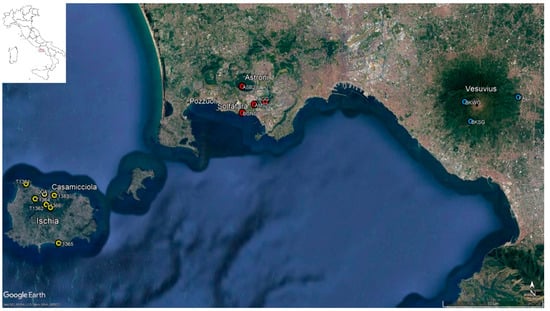
Figure 1.
Map of the Neapolitan volcanoes (Vesuvius, Campi Flegrei, and Ischia) with the seismic stations (circles in blue for Vesuvius, red for Campi Flegrei, and yellow for Ischia) used for the analysis.
For the Campi Flegrei caldera, we selected data recorded in 2006, when a relevant low-frequency hydrothermal component in the background seismic signal was evidenced by [36] and interpreted as related to fluid injections from a deeper geothermal reservoir toward the shallower hydrothermal system of the Solfatara. On Ischia, we considered samples recorded after the Mw 3.9 earthquake, which occurred on 21 August 2017, when the hydrothermal source was particularly active and its persistent signature was identified in background noise [9,25]. At Vesuvius, the seismic noise was (randomly) sampled during the first months of 2019. At Colima volcano, data were collected in 2006, during a temporary seismic survey organized by the Istituto Nazionale di Geofisica e Vulcanologia (INGV)–Osservatorio Vesuviano, the Observatorio Vulcanologico de Colima of Colima University (OVC) and the Instituto Andaluz de Geofisica (IAG), University of Granada, Spain [51]. We used seismograms recorded by three digital seismic stations (COME, COCA, and COBA) consisting of broadband three-component seismometers Lennartz LE-3D/20 s; the sampling rate was at 62.5 Hz. A map with the location of the stations and the investigated area (Colima volcano) is reported in Figure 2.
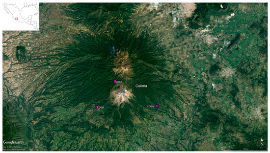
Figure 2.
Map of Colima volcano with the seismic stations (magenta circles) (map data ©2021 Google).
2.3. Machine Learning Approach
The role of machine learning approaches in volcanic seismology has widely increased in the last decades, especially with the constantly increasing volumes of seismic data and the limitations of manual classification [52]. Volcano-seismic signal classification is a crucial component of volcanic monitoring, accomplished by using several ML methods, such as multi-layer perceptrons [29,30,34], cluster analysis [53], self-organizing maps [32], support vector machines [54], and even Bayesian belief networks for assessing the seismic soil liquefaction potential [55,56,57].
A crucial role has been played by the multi-layer perceptrons, widely employed for earthquake prediction [26,58]. It is a feed-forward neural network, consisting of three layers: an input, hidden, and output layer. Data flow forward from the input layer to the output layer. The neurons are fully connected; that is, each node in one layer is connected to each node in the next layer. An arbitrary number of hidden layers, placed between the input and output layers, form the computational engine of the MLP. The neurons of the MLP are trained with the back-propagation algorithm, which modifies the internal state to reduce the error between the model output and the expected output. MLPs are designed to approximate any continuous function and can solve nonlinearly separable problems. The need to process an increasing volume of data, with no degradation in terms of efficiency, finds in the deep neural networks (DNNs) an effective predictive model with multiple hidden layers between the input and output. DNNs can discover intrinsic patterns within large datasets and fine-tune their internal parameters in each layer using the back-propagation algorithm. In volcanic seismology, MLPs have been widely used for classification of seismic events, although recent studies have focused on specialized deep neural networks, such as convolutional neural networks [34] or recurrent neural networks [31], capable of processing large amounts of seismic data; in particular, CNNs have found wide use for earthquake detection [59] or classification of seismic events [34].
In the light of these observations, the workflow in Figure 3 sketches the overall process to automatically classify the background noise signals.
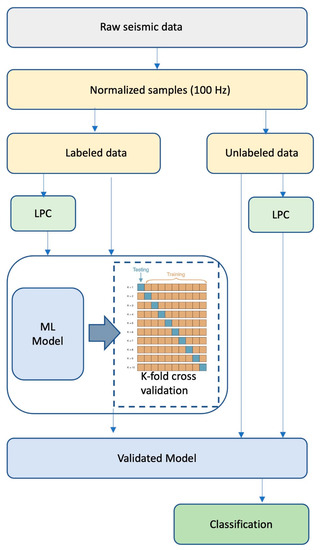
Figure 3.
Workflow of the ML process.
Figure 3 shows the dataflow of our high-level processing for noise background classification. The raw data, i.e., the background seismic signals from the presented volcanoes, are preprocessed, splitting it into separate time windows lasting 24 s (20 s devoted to the event signal and 4 s due to the overlapping windows). Due to the different types of acquisitors gathered from the stations, the raw signals were resampled at 100 Hz to get the sample normalization. This normalization process is described in [34]. The samples are separated into two parts: one for ML model training and validation and the other part called unlabeled data is the unseen signals that will be classified by the ML model once trained.
Then, depending on the ML model employed, the normalized raw data (labeled data) are further processed or not, before being given as input to the model. Precisely, in the case of the MLP model, the data are preprocessed by linear predictive coding (LPC) filtering, which is widely used for signal processing [60,61] to extract relevant features, while in the CNN approach, the raw data are input. Similarly, the unlabeled data may be preprocessed or not, depending on the classification model selected. Therefore, in Figure 3, LPC filtering must also be performed on the unlabeled data if they are given as input to the MLP model.
The labeled data are validated by (stratified) k-fold cross-validation, to guarantee a reliable and robust classification model. Cross-validation, indeed, allows for improving the flexibility of a model and thus the performance of the proposed model. The method splits the dataset into ‘k’ sub-samples, in which one sample is used for testing and the remaining k-1 dataset is used for training purposes. The whole process is repeated k times by varying the training samples and testing samples. After the k iterations, the best instance of the model (i.e., validated model) is selected and used for the classification of unlabeled data.
As stated, the workflow of Figure 3 has been accomplished and validated with two instances of the ML models, namely MLP and CNN.
Our MLP is a layered feedforward neural network with back-propagation algorithm [62], described in terms of the stochastic gradient descent algorithm, and it minimizes the categorical cross-entropy loss function. The activation function used for the hidden layer is ReLU (rectified linear unit), while the softmax function is used in the output layer. Other training parameter configurations of MLP are reported as follows.
- Hidden layer size: 42;
- Number of samples by iteration: 50;
- Learning rate: 0.001;
- Gradient direction: 0.9;
- Epochs: 320.
Let us notice that the raw data are preprocessed from linear predictive coding (LPC) to extract spectral features and, in addition, a discretized waveform parameterization of signals composed of 24 s windows is also considered as further input features, as proposed in [34]. The total number of features is 80: 56 spectral features from the LPC (using 8 subwindows of 3 s and setting the order equal to 6), and 24 waveform features from the discrete waveform parametrization.
The second ML model is based on CNN [63], becoming a de facto standard for many applications in computer vision and machine learning [64,65]. The method has been widely used in characterizing signals in any research field, especially those oriented to biomedical applications [61]. Herein, a one-dimensional convolutional neural, 1D CNN, has been employed; it has become a popular choice among ML researchers for the significant complexity reduction against the 2D CNN, reducing the computing times, and being used in real-time and low-cost applications. In particular, 1D CNN methods are used for processing time-series data or, particularly, for patient-specific ECG signals in the biomedical domain [66]. In our case, Figure 4 shows our 1D CNN.
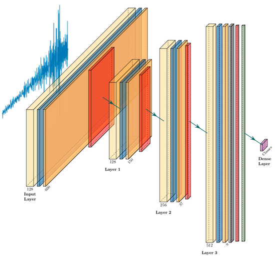
Figure 4.
CNN architecture design with the colored layers. Yellow: convolution 1D; blue: batch normalization; orange: activation (ReLu); red: MaxPooling1D; gray: dropout (50%); light green: Lambda (mean); and purple: dense (softmax).
The proposed CNN is composed of four-layer blocks; each block includes a convolution one-dimension layer, the batch normalization operation, the ReLU activation function, and, finally, a MaxPooling operation. As shown in Figure 4, the initial convolutional layer has 128 filters used for our time-series data of size 2400, a kernel size of 80, and a stride of 4. The Xavier (also known as Glorot) uniform initializer was used to randomly initialize the weights of the layer. This block structure appears three times but with 128, 128, and 256 filters, respectively, in the layers called input layer, layer 1, and layer 2 in Figure 4. Layer 1 and layer 2 have instead a kernel size of 3 and stride 1. Finally, layer 3 has a similar design but uses 512 filters, with a kernel size 3 and stride 1. This last block also provides a dropout layer with 50% probability to avoid overfitting along with a Lambda “mean” layer. Finally, a dense layer with softmax activation provides a three-neurons output layer. The proposed CNN model architecture traced approximately 558,597 parameters on the samples trained to perform the classification.
The parameter configuration of 1D CNN is chosen as follows.
- Layers: 4:
- ○
- Filters: 128, 128, 256, 512 (respectively),
- ○
- Kernel initializer: Glorot uniform,
- ○
- Activation function: rectification linear unit (ReLU);
- Epochs: 200;
- Dropout: 50%;
- Last layer activation function: softmax;
- Loss function: categorical cross-entropy;
- Optimizer: Adam;
- Callbacks: ReduceLROnPlateau;
- ○
- Monitor: ’val loss’
- ○
- Patience: 5
- ○
- Reduction Factor: 0.1
- ○
- Learning Rate: 0.0001
3. Results
3.1. Spectral Analysis
We performed a spectral analysis on the data samples to characterize the seismic noise recorded at each volcano in terms of its frequency content.
Examples of waveforms of the seismic noise recorded at the Neapolitan and Colima volcanoes are shown in Figure 5 and Figure S1–S5. As one can observe, the noise has different amplitude levels and frequencies depending on the volcano, on the specific site where the station is located, and on the component of motion.
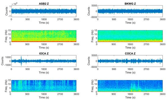
Figure 5.
Examples of vertical component recordings of seismic noise and corresponding spectrograms, at Campi Flegrei (ASB2 station), Ischia (IOCA station), Vesuvius (BKSG station), and Colima (COCA station).
The spectral features are summarized in Table 1, where we report the frequency range of the main spectral peaks and their possible origin according to the framework described in the Seismological Overview section. Some considerations arise from this analysis: microseism caused by sea loading (<1 Hz) is observed at all the volcanoes but in two cases it is mixed with the contribution related to hydrothermal (Campi Flegrei) or volcanic (Colima) sources. Anthropogenic noise is usually recorded above the frequency of 1 Hz up to 12–15 Hz, but the specific ranges depend on the volcano and on the site. Moreover, in the case of Ischia, part of the anthropogenic frequency band (1–5 Hz) is superimposed with that of the hydrothermal signal. Finally, at the Neapolitan volcanoes, the effect of human activities on the background seismic signal is strong because the seismic stations are installed in densely urbanized areas. In contrast, this effect is minimal (or even practically absent) at the Colima volcano, where the seismic stations were installed in a sparsely populated region.

Table 1.
Characterization of the frequency content of the seismic noise recorded at the Campi Flegrei, Ischia, Vesuvius, and Colima volcanoes. The interpretation of the origin of the spectral peaks is based on the works described in the Seismological Overview subsection.
3.2. Machine Learning-Based Processing
The seismic data used for training the proposed ML architectures consist of 83,147 pre-labeled events, of which 75,133 samples are from background noise signals acquired at the four volcanoes. They represent the most consistent part of the dataset, used to train our ML models; to improve the efficacy of the ML methods, an additional 8014 samples from known events, i.e., LPs, VTs, quarry blasts, and undersea explosions, recorded by seismic sensor networks are added to the dataset. These transient events can be considered a sort of variability and heterogeneity to assess the ML-based classification performances.
Let us recall that for MLP training, seismic events have been preprocessed using LPC for extracting spectral features [60,61], as well as signal parametrization to obtain waveform information [29], so the input vector for MLP model is composed of 80 components for each signal. Instead, the raw data, i.e., 24 s windowed signals, were used to train the CNN 1D model, with no data preprocessing.
Starting from the results presented in [34], two experiments have been introduced aimed at the detection and classification of the background noise signals. The first experiment was carried out on all the background noise signals. The ML methods were trained to distinguish among the noise signals at the different sources used. As reported in Table 2, four classes of signals have been considered; the dataset results are balanced, since each class is approximately composed of the same number of signals. The second experiment has the same classes reported in the first experiment, with one more composed of transients, i.e., VTs, LPs, quarry blasts, and undersea explosions [34]. This class represents a set of “no background signals” used to validate the ML method’s capability to learn and classify noise signals.
Table 2.
Experiment setting: class sizes associated with each background noise source.
Our goal in both experiments is to discriminate the volcano fingerprint (in the stationary phase) across the background noise also in the presence of higher energy transient events.
The performance evaluation for the MLP and CNN methods are calculated considering the known metrics, namely precision (P), recall (R), F1 score (F1), and accuracy (Acc). These measures are based on the evaluation of the following parameters:
- –
- tp (true positive): is the number of samples correctly assigned to a class.
- –
- tn (true negative) is the number of samples correctly not assigned to a given class.
- –
- fp (false positive) is the number of samples wrongly assigned to a class.
- –
- fn (false negative) is the number of samples wrongly not assigned to a given class.
More precisely, these metrics are reported in Table 3: the precision describes how precise/accurate our model is out of those predicted positives; the recall calculates how many of the actual correctly classified our model captures by labeling them as true positives. The F1 score is the weighted average of precision and recall, while the accuracy is the simplest metrics, providing a ratio of correctly classified samples to the total sample dataset.
Table 3.
Precision, recall, F1 score, and accuracy definitions.
The experiment results can be seen in Table 4 for the two models employed, namely, MLP and CNN. According to the workflow sketched in Figure 3, the models have been validated by using a 10-fold cross-validation technique. Precisely, for the second experiment proposing unbalanced class samples (the “Event” class is smaller than the others), a stratified k-fold algorithm from Python Scikit-learn library was carried out to enforce the class distribution in each split of the data to match the distribution in the complete training dataset.
Table 4.
Average accuracy, precision, recall, and F1 score of the two models, evaluated for the two experiments.
The table shows the mean and the standard deviation of accuracy results for the training data and loss, as well as for testing data. The mean and the standard deviation are also provided for P, R, and F1. As reported, the performance of the results of the two ML models are quite satisfactory: with the MLP model, Experiment 1 provides better performance than Experiment 2, which involves not only the background signals but also additional transient signals. The latter are different from the background signals of the predefined classes, used in some sense to “dirty” the dataset to evaluate the ability of the model in discriminating extraneous transient events from the background signals to be classified.
Similar behavior appears for the CNN model, whose performance in the case of Experiment 1 is very promising since the values of both accuracy and F1 are close to 100%. This result emphasizes how CNN is able to correctly discriminate between balanced classes of noise signals. In the case of Experiment 2, instead, a certain unbalance in the class distribution reflects in the results returned by the model, with a significant standard deviation value for the accuracy. The F1 score, although assuming a similar value to accuracy, is more stable (i.e., the standard deviation is low), according to its characteristic to work better with unbalanced classes.
The concatenated confusion matrices computed by considering the predictions for test data in each fold by cross-validation are also reported in Table 5, according to the model used and for each experiment. The confusion matrices confirm the observations reported above, highlighting the satisfying performance of the CNN model in both experiments.
Table 5.
Normalized confusion matrices for the MLP and CNN models for the two experiments.
4. Discussion and Conclusions
In the framework of forecasting volcanic eruptions, much attention is generally devoted to the analysis of seismic transients for a prompt detection and cataloging of the waveforms. The reason is the strict link between the dynamical state of a volcano and the seismic signals such as LPs or VTs. On the other hand, seismic acquisition is a complex superposition of several signals emitted by different sources, which can be internal or external to a volcano, that can share common properties, especially the frequency content, making the discrimination even more difficult.
Here, we demonstrate that it is possible to recognize the fingerprint of a specific volcano by basically analyzing the background seismic noise, taking advantage of continuous acquisition in a stationary volcanic phase. This puts on a more quantitative basis the now consolidated idea that persistent tremor, both volcanic and hydrothermal, and some volcanic transients (i.e., LPs or explosion quakes) are generated by the same physical mechanism, eventually in different regimes involving different levels of seismic energy.
Investigations were conducted by using ML techniques for the Neapolitan volcanoes and the Colima volcano. These analyses are advantageous in cases of weak ground motions as the background seismic noise, which is plenty of information often neglected by traditional signal processing techniques. The ML-based models provide very reliable solutions when all the traces of all the volcanoes are mixed together, allowing the identification of pieces of background tremor. But more than this, our method ascribes each recognized tremor to the relative volcano with its own characteristics. In addition, introducing new classes of labeled noise waveforms in the framework of ML techniques allows enriching the training phases so that the classifier can better discriminate among low-energy volcanic signals from spurious ones, just reducing the probability to detect false positive events [35]. The accurate identification and classification of continuous seismic noise represent progress toward the characterization of background signals, which can also be implemented in real-time for monitoring purposes.
The promising performance shown by our ML approach in background noise analysis applied to volcanoes with different activities (e.g., hydrothermal, volcanic, anthropogenic, etc.), in quiescent or in unrest phases, and with even different geological features (calderas, stratovolcano), makes us confident that the method can be extended to a large variety of volcanoes for extracting their fingerprints and significantly contributing to the study of the seismic/volcanic sources.
Separate classification of background noise and transients opens the way to hybrid approaches that use specific classifiers, integrated into decision models to employ both signals, even constructed from a dataset provided by a single seismic station. This would be successful in those areas that are not accessible to locate seismic networks or seismic arrays. Finally, our network should recognize any anomalies in the background noise, thus indirectly evidencing changes in the dynamics of a volcano.
Supplementary Materials
The following supporting information can be downloaded at: https://www.mdpi.com/article/10.3390/app12146835/s1, Figure S1: Examples of seismic noise three-component (Z = vertical, N = north-south, E = east-west) seismograms and corresponding spectrograms recorded at stations ASB2, AMS2, TAGG, and BGNG located at Campi Flegrei. Figure S2: Examples of seismic noise three-component (Z = vertical, N = north-south, E = east-west) seismograms and corresponding spectrograms recorded at stations IOCA, T1363, and T1364 located at Ischia. Figure S3: Examples of seismic noise three-component (Z = vertical, N = north-south, E = east-west) seismograms and corresponding spectrograms recorded at stations T1361, T1362, and T1365 located at Ischia. Figure S4: Examples of seismic noise three-component (Z = vertical, N = north-south, E = east-west) seismograms and corresponding spectrograms recorded at stations BKWG, BKSG, and FAL2 located at Vesuvius. Figure S5: Examples of seismic noise three-component (Z = vertical, N = north-south, E = east-west) seismograms and corresponding spectrograms recorded at stations COCA, COBA, and COME located at Colima.
Author Contributions
Conceptualization, M.F.; methodology, D.R.-Y. and S.S.; investigation, D.R-Y. and S.P.; data curation, S.P.; writing—original draft preparation, M.F. and S.P.; writing—review and editing, E.D.L., M.F., D.R.-Y., S.P. and S.S. All authors have read and agreed to the published version of the manuscript.
Funding
This research received no external funding.
Institutional Review Board Statement
Not applicable.
Data Availability Statement
Data are available upon request.
Acknowledgments
We acknowledge the “Istituto Nazionale di Geofisica e Vulcanologia, Sez. Napoli—Osservatorio Vesuviano” for providing the seismic dataset of Ischia, Campi Flegrei, and Vesuvius. We thank the “Istituto Nazionale di Geofisica e Vulcanologia (INGV)–Sez. Osservatorio Vesuviano”, the “Observatorio Vulcanologico de Colima of Colima University (OVC)” and the “Instituto Andaluz de Geofisica (IAG)”, University of Granada, Spain for the seismic data of the Colima volcano.
Conflicts of Interest
The authors declare no conflict of interest.
References
- Bormann, P.; Wielandt, E. Seismic signals and noise. In New Manual of Seismological Observatory Practice 2 (NMSOP2); Deutsches GeoForschungsZentrum GFZ: Potsdam, Germany, 2013; pp. 1–62. [Google Scholar]
- Groos, J.C.; Ritter, J.R.R. Time domain classification and quantification of seismic noise in an urban environment. Geophys. J. Int. 2009, 179, 1213–1231. [Google Scholar] [CrossRef]
- De Lauro, E.; De Martino, S.; Falanga, M.; Palo, M.; Scarpa, R. Evidence of VLP volcanic tremor in the band [0.2–0.5] Hz at Stromboli volcano, Italy. Geophys. Res. Lett. 2005, 32. [Google Scholar] [CrossRef]
- Capuano, P.; De Lauro, E.; De Martino, S.; Falanga, M.; Petrosino, S. Convolutive independent component analysis for processing massive datasets: A case study at Campi Flegrei (Italy). Nat. Hazards 2017, 86, 417–429. [Google Scholar] [CrossRef]
- Poli, P.; Boaga, J.; Molinari, I.; Cascone, V.; Boschi, L. The 2020 coronavirus lockdown and seismic monitoring of anthropic activities in Northern Italy. Sci. Rep. 2020, 10, 9404. [Google Scholar] [CrossRef] [PubMed]
- Stutzmann, E.; Roult, G.; Astiz, L. GEOSCOPE station noise levels. Bull. Seismol. Soc. Am. 2000, 90, 690–701. [Google Scholar] [CrossRef]
- Saccorotti, G.; Maresca, R.; Del Pezzo, E. Array analyses of seismic noise at Mt. Vesuvius Volcano, Italy. J. Volcanol. Geotherm. Res. 2001, 110, 79–100. [Google Scholar] [CrossRef]
- Ciaramella, A.; De Lauro, E.; Falanga, M.; Petrosino, S. Automatic detection of long-period events at Campi Flegrei caldera (Italy). Geophys. Res. Lett. 2011, 38. [Google Scholar] [CrossRef]
- Cusano, P.; Petrosino, S.; De Lauro, E.; Falanga, M. The whisper of the hydrothermal seismic noise at Ischia Island. J. Volcanol. Geotherm. Res. 2020, 389, 106693. [Google Scholar] [CrossRef]
- Bey, N.Y. Extraction of signals buried in noise, part I: Fundamentals. Signal Process 2006, 86, 2464–2478. [Google Scholar] [CrossRef]
- Bey, N.Y. Extraction of signals buried in noise, part II: Experimental results. Signal Process 2006, 86, 2994–3011. [Google Scholar] [CrossRef]
- Meng, H.; Ben-Zion, Y.; Johnson, C.W. Detection of random noise and anatomy of continuous seismic waveforms in dense array data near Anza California. Geophys. J. Int. 2019, 219, 1463–1473. [Google Scholar] [CrossRef]
- Soubestre, J.; Seydoux, L.; Shapiro, N.M.; De Rosny, J.; Droznin, D.V.; Droznina, S.Y.; Senyukov, S.L.; Gordeev, E.I. Depth migration of seismovolcanic tremor sources below the Klyuchevskoy volcanic group (Kamchatka) determined from a network-based analysis. Geophys. Res. Lett. 2019, 46, 8018–8030. [Google Scholar] [CrossRef]
- De Lauro, E.; De Martino, S.; Del Pezzo, E.; Falanga, M.; Palo, M.; Scarpa, R. Model for high-frequency Strombolian tremor inferred by wavefield decomposition and reconstruction of asymptotic dynamics. J. Geophys. Res. Solid Earth 2008, 113. [Google Scholar] [CrossRef]
- Falanga, M.; Petrosino, S. Inferences on the source of long-period seismicity at Campi Flegrei from polarization analysis and reconstruction of the asymptotic dynamics. Bull. Volcanol. 2012, 74, 1537–1551. [Google Scholar] [CrossRef]
- Ibáñez, J.; Del Pezzo, E.; Almendros, J.; La Roccam, M.; Alguacil, G.; Ortiz, R.; García, A. Seismovolcanic signals at Deception Island volcano, Antarctica: Wave field analysis and source modeling. J. Geophys. Res. 2000, 105, 13905–13931. [Google Scholar] [CrossRef]
- Lesage, P.; Mora, M.; Alvarado, G.; Pacheco, J.; Métaxian, J.P. Complex behavior and source model of the volcanic tremor at Arenal volcano, Costa Rica. J. Volcanol. Geoth. Res. 2006, 157, 49–59. [Google Scholar] [CrossRef]
- Almendros, J.; Abella, R.; Mora, M.M.; Lesage, P. Array analysis of the seismic wavefield of long-period events and volcanic tremor at Arenal Volcano, Costa Rica. J. Geophys. Res. Solid Earth 2014, 119, 5536–5559. [Google Scholar] [CrossRef]
- Chouet, B.; Saccorotti, G.; Martini, M.; Dawson, P.; De Luca, G.; Milana, G.; Scarpa, R. Source and path effects in the wave fields of tremor and explosions at Stromboli Volcano, Italy. J. Geophys. Res. 1997, 102, 15129–15150. [Google Scholar] [CrossRef]
- Yukutake, Y.; Honda, R.; Harada, M.; Doke, R.; Saito, T.; Ueno, T.; Sakai, S.I.; Morita, Y. Analyzing the continuous volcanic tremors detected during the 2015 phreatic eruption of the Hakone Volcano. Earth Planets Space 2017, 69, 164. [Google Scholar] [CrossRef]
- De Lauro, E.; De Martino, S.; Falanga, M.; Palo, M. Modelling the macroscopic behavior of Strombolian explosions at Erebus volcano. Phys. Earth Planet. Inter. 2009, 176, 174–186. [Google Scholar] [CrossRef][Green Version]
- Barriere, J.; Oth, A.; Theys, N.; d’Oreye, N.; Kervyn, F. Long-term monitoring of long-period seismicity and space-based SO2 observations at African lava lake volcanoes Nyiragongo and Nyamulagira (DR Congo). Geophys. Res. Lett. 2017, 44, 6020–6029. [Google Scholar] [CrossRef]
- Caudron, C.; Taisne, B.; Kugaenko, Y.; Saltykov, V. Magma migration at the onset of the 2012–13 Tolbachik eruption revealed by seismic amplitude ratio analysis. J. Volcanol. Geotherm. Res. 2015, 307, 60–67. [Google Scholar] [CrossRef]
- Woods, J.; Donaldson, C.; White, R.S.; Caudron, C.; Brandsdóttir, B.; Hudson, T.S.; Ágústsdóttir, T. Long-period seismicity reveals magma pathways above a laterally propagating dyke during the 2014–15 Bárdarbunga rifting event, Iceland. Earth Planet. Sci. Lett. 2018, 490, 216–229. [Google Scholar] [CrossRef]
- Falanga, M.; Cusano, P.; De Lauro, E.; Petrosino, S. Picking up the hydrothermal whisper at Ischia Island in the COVID-19 lockdown quiet. Sci. Rep. 2021, 11, 8871. [Google Scholar] [CrossRef]
- Bianco, F.; Cusano, P.; Petrosino, S.; Castellano, M.; Buonocunto, C.; Capello, M.; Del Pezzo, E. Small-aperture array for seismic monitoring of Mt. Vesuvius. Seismol. Res. Lett. 2005, 76, 344–355. [Google Scholar] [CrossRef]
- Varley, N.; Connor, C.B.; Komorowski, J.-C. Volcan de Colima: Portrait of a Persistently Hazardous Volcano; Springer: Berlin/Heidelberg, Germany, 2019. [Google Scholar]
- Permana, T.; Nishimura, T.; Nakahara, H.; Shapiro, N. Classification of volcanic tremors and earthquakes based on seismic correlation: Application at Sakurajima volcano, Japan. Geophys. J. Int. 2022, 229, 1077–1097. [Google Scholar] [CrossRef]
- Scarpetta, S.; Giudicepietro, F.; Ezin, E.C.; Petrosino, S.; Del Pezzo, E.; Martini, M.; Marinaro, M. Automatic classification of seismic signals at Mt. Vesuvius volcano, Italy, using neural networks. Bull. Seismol. Soc. Am. 2005, 95, 185–196. [Google Scholar] [CrossRef]
- Rincon-Yanez, D.; De Lauro, E.; Falanga, M.; Senatore, S.; Petrosino, S. Towards a semantic model for IoT-based seismic event detection and classification. In Proceedings of the 2020 IEEE Symposium Series on Computational Intelligence (SSCI), Canberra, ACT, Australia, 1–4 December 2020; pp. 189–196. [Google Scholar]
- Titos, M.; Bueno, A.; Garcıa, L.; Benıtez, C.; Segura, J.C. Classification of isolated volcano-seismic events based on inductive transfer learning. IEEE Geosci. Remote Sens. Lett. 2020, 17, 869–873. [Google Scholar] [CrossRef]
- Carniel, R.; Guzmán, S.R. Machine Learning in Volcanology: A Review. In Updates in Volcanology—Transdisciplinary Nature of Volcano Science; Németh, K., Ed.; IntechOpen: London, UK, 2020. [Google Scholar] [CrossRef]
- Moran, S.C.; Freymueller, J.T.; LaHusen, R.G.; McGee, K.A.; Poland, M.P.; Power, J.A.; Schmidt, D.A.; Schneider, D.J.; Stephens, G.; Werner, C.A.; et al. Instrumentation Recommendations for Volcano Monitoring at U.S. Volcanoes under the National Volcano Early Warning System: U.S. Geological Survey Scientific Investigations Report 2008-5114; U.S. Department of the Interior: Washington, DC, USA; U.S. Geological Survey: Reston, VA, USA, 2008; 47p.
- Falanga, M.; De Lauro, E.; Petrosino, S.; Rincon-Yanez, D.; Senatore, S. Semantically enhanced IoT-oriented seismic event detection: An application to Colima and Vesuvius volcanoes. IEEE Internet Things J. 2022, in press. [Google Scholar] [CrossRef]
- Johnson, C.W.; Ben-Zion, Y.; Meng, H.; Vernon, F. Identifying different classes of seismic noise signals using unsupervised learning. Geophys. Res. Lett. 2020, 47, e2020GL088353. [Google Scholar] [CrossRef]
- De Lauro, E.; De Martino, S.; Falanga, M.; Petrosino, S. Synchronization between tides and sustained oscillations of the hydrothermal system of Campi Flegrei (Italy). Geochem. Geophys. Geosystems 2013, 14, 2628–2637. [Google Scholar] [CrossRef]
- Petrosino, S.; Cusano, P.; Madonia, P. Tidal and hydrological periodicities of seismicity reveal new risk scenarios at Campi Flegrei caldera. Sci. Rep. 2018, 8, 13808. [Google Scholar] [CrossRef] [PubMed]
- Kieffer, S.W. Seismicity of Old Faithful geyser: An isolated source of geothermal noise and possible analogue of volcanic seismicity. J. Volcanol. Geotherm. Res. 1984, 22, 59–95. [Google Scholar] [CrossRef]
- Gottsmann, J.; Carniel, R.; Coppo, N.; Wooller, L.; Hautmann, S.; Rymer, H. Oscillations in hydrothermal systems as a source of periodic unrest at caldera volcanoes: Multiparameter insights from Nisyros, Greece. Geophys. Res. Lett. 2007, 34, L07307. [Google Scholar] [CrossRef]
- Petrosino, S.; Damiano, N.; Cusano, P.; Di Vito, M.A.; de Vita, S.; Del Pezzo, E. Subsurface structure of the Solfatara volcano (Campi Flegrei caldera, Italy) as deduced from joint seismic-noise array, volcanological and morphostructural analysis. Geochem. Geophys. Geosyst. 2012, 13, Q07006. [Google Scholar] [CrossRef]
- Petrosino, S.; Dumont, S. Tidal modulation of hydrothermal tremor: Examples from Ischia and Campi Flegrei volcanoes, Italy. Front. Earth Sci. 2022, 9, 775269. [Google Scholar] [CrossRef]
- Isaia, R.; Di Giuseppe, M.G.; Natale, J.; Tramparulo, F.D.; Troiano, A.; Vitale, S. Volcano-tectonic setting of the Pisciarelli Fumarole field, Campi Flegrei Caldera, Southern Italy: Insights into fluid circulation patterns and hazard scenarios. Tectonics 2021, 40, e2020TC006227. [Google Scholar] [CrossRef]
- Cusano, P.; Caputo, T.; De Lauro, E.; Falanga, M.; Petrosino, S.; Sansivero, F.; Vilardo, G. Tracking the Endogenous Dynamics of the Solfatara Volcano (Campi Flegrei, Italy) through the Analysis of Ground Thermal Image Temperatures. Atmosphere 2021, 12, 940. [Google Scholar] [CrossRef]
- De Lauro, E.; De Martino, S.; Falanga, M.; Petrosino, S. Fast wavefield decomposition of volcano-tectonic earthquakes into polarized P and S waves by Independent Component Analysis. Tectonophysics 2016, 690, 355–361. [Google Scholar] [CrossRef]
- Ricco, C.; Petrosino, S.; Aquino, I.; Cusano, P.; Madonia, P. Tracking the recent dynamics of mt. Vesuvius from joint investigations of ground deformation, seismicity and geofluid circulation. Sci. Rep. 2021, 11, 965. [Google Scholar] [CrossRef]
- Petrosino, S.; Cusano, P. Low frequency seismic source investigation in volcanic environment: The mt. Vesuvius atypical case. Adv. Geosci. 2020, 52, 29–39. [Google Scholar] [CrossRef]
- Zobin, V.M.; Orozco-Rojas, J.; Reyes-D’Avila, G.A.; Navarro, C. Seismicity of an andesitic volcano during block-lava effusion: Volcan de Colima, Mexico, November 1998–January 1999. Bull. Volcanol. 2005, 67, 679–688. [Google Scholar] [CrossRef]
- De Lauro, E.; De Martino, S.; Palo, M.; Ibanez, J. Self-sustained oscillations at Volcan de Colima (Mexico) inferred by Independent Component Analysis. Bull. Volcanol. 2012, 74, 279–292. [Google Scholar] [CrossRef]
- Palo, M.; Cusano, P. Wavefield decomposition and phase space dynamics of the seismic noise at Volcàn de Colima, Mexico: Evidence of a two-state source process. Nonlinear Processes Geophys. 2013, 20, 71–84. [Google Scholar] [CrossRef][Green Version]
- La Rocca, M.; Galluzzo, D. Seismic monitoring of Campi Flegrei and Vesuvius by stand-alone instruments. Ann. Geophys. 2015, 58, 1–14. [Google Scholar] [CrossRef]
- Petrosino, S.; Cusano, P.; La Rocca, M.; Galluzzo, D.; Orozco-Rojas, J.; Bretón, M.; Ibáñez, J.; Del Pezzo, E. Source location of long period seismicity at Volcàn de Colima, México. Bull. Volcanol. 2011, 73, 887–898. [Google Scholar] [CrossRef]
- Malfante, M.; Dalla Mura, M.; Mars, J.I.; Métaxian, J.P.; Macedo, O.; Inza, A. Automatic classification of volcano seismic signatures. J. Geophys. Res. Solid Earth 2018, 123, 10645–10658. [Google Scholar] [CrossRef]
- Ren, C.X.; Peltier, A.; Ferrazzini, V.; Rouet-Leduc, B.; Johnson, P.; Brenguier, F. Machine learning reveals the seismic signature of eruptive behavior at piton de la fournaise volcano. Geophys. Res. Lett. 2020, 47, e2019GL085523. [Google Scholar] [CrossRef]
- Masotti, M.; Falsaperla, S.; Langer, H.; Spampinato, S.; Campanini, R. Application of Support Vector Machine to the classification of volcanic tremor at Etna, Italy. Geophys. Res. Lett. 2006, 33. [Google Scholar] [CrossRef]
- Mahmood, A.; Tang, X.W.; Qiu, J.N.; Ahmad, F.; Gu, W.J. Application of machine learning algorithms for the evaluation of seismic soil liquefaction potential. Front. Struct. Civ. Eng. 2021, 15, 490–505. [Google Scholar]
- Mahmood, A.; Tang, X.W.; Qiu, J.N.; Gu, W.J.; Feezan, A. A hybrid approach for evaluating CPT-based seismic soil liquefaction potential using Bayesian belief networks. J. Cent. South Univ. 2020, 27, 500–516. [Google Scholar] [CrossRef]
- Tang, S.B.; Dong, Z.; Wang, J.X.; Mahmood, A. A numerical study of fracture initiation under different loads during hydraulic fracturing. J. Cent. South Univ. 2020, 27, 3875–3887. [Google Scholar] [CrossRef]
- Reyes, J.; Morales-Esteban, A.; Martínez-Álvarez, F. Neural networks to predict earthquakes in Chile. Appl. Soft Comput. 2013, 13, 1314–1328. [Google Scholar] [CrossRef]
- Zhu, W.; Beroza, G.C. PhaseNet: A deep neural-network-based seismic arrival-time picking method. Geophys. J. Int. 2019, 216, 261–273. [Google Scholar] [CrossRef]
- O’Shaughnessy, D. Linear predictive coding. IEEE Potentials 1988, 7, 29–32. [Google Scholar] [CrossRef]
- Gadermayr, M.; Dombrowski, A.K.; Klinkhammer, B.M.; Boor, P.; Merhof, D. CNN cascades for segmenting sparse objects in gigapixel whole slide images. Comput. Med. Imaging Graph. 2019, 71, 40–48. [Google Scholar] [CrossRef]
- Irie, B.; Miyake, S. Capabilities of three-layered perceptrons. In Proceedings of the IEEE 1988 International Conference on Neural Networks, San Diego, CA, USA, 24–27 July 1988; pp. 641–648. [Google Scholar]
- LeCun, Y.; Bengio, Y.; Hinton, G. Deep learning. Nature 2015, 521, 436–444. [Google Scholar] [CrossRef]
- Russakovsky, O.; Deng, J.; Su, H.; Krause, J.; Satheesh, S.; Ma, S.; Huang, Z.; Karpathy, A.; Khosla, A.; Bernstein, M.; et al. Imagenet large scale visual recognition challenge. Int. J. Comput. Vis. 2015, 115, 211–252. [Google Scholar] [CrossRef]
- Girshick, R. Fast r-cnn. In Proceedings of the IEEE International Conference on Computer Vision (ICCV), Santiago, Chile, 11–18 December 2015; pp. 1440–1448. [Google Scholar]
- Kiranyaz, S.; Avci, O.; Abdeljaber, O.; Ince, T.; Gabbouj, M.; Inman, D.J. 1D convolutional neural networks and applications: A survey. Mech. Syst. Signal Process. 2021, 151, 107398. [Google Scholar] [CrossRef]


Publisher’s Note: MDPI stays neutral with regard to jurisdictional claims in published maps and institutional affiliations. |
© 2022 by the authors. Licensee MDPI, Basel, Switzerland. This article is an open access article distributed under the terms and conditions of the Creative Commons Attribution (CC BY) license (https://creativecommons.org/licenses/by/4.0/).