A Surrogate Model Based Multi-Objective Optimization Method for Optical Imaging System

Abstract

An optimization model for the optical imaging system was established in this paper. It combined the modern design of experiments (DOE) method known as Latin hypercube sampling (LHS), Kriging surrogate model training, and the multi-objective optimization algorithm NSGA-III into the optimization of a triplet optical system. Compared with the methods that rely mainly on optical system simulation, this surrogate model-based multi-objective optimization method can achieve a high-accuracy result with significantly improved optimization efficiency. Using this model, case studies were carried out for two-objective optimizations of a Cooke triplet optical system. The results showed that the weighted geometric spot diagram and the maximum field curvature were reduced 5.32% and 11.59%, respectively, in the first case. In the second case, where the initial parameters were already optimized by Code-V, this model further reduced the weighted geometric spot diagram and the maximum field curvature by another 3.53% and 4.33%, respectively. The imaging quality in both cases was considerably improved compared with the initial design, indicating that the model is suitable for the optimal design of an optical system.

1. Introduction

The optimal design of an optical imaging system [1,2] is a vital problem for designing modern complex optical equipment. In the past, the optimization of optical systems relied mainly on the engineers’ experience, which can only provide very limited guidance for the optimal design of some modern optical equipment. The design space of an optical imaging system is decided by the number and the variance of desired design parameters. With the optical system becoming more and more complex, the modern optimal design has developed into a process heavily relying on computer calculation to find an optimal point/solution in a design space with high dimensionality. The difficulty of this process is often affected by the number of required design parameters, the variance of these parameters, and the acceptable tolerance of the optimal design solution.

With the increase in a design space’s dimension, the successful search for an optimal point for both local and global optimization algorithms becomes more and more difficult. With a rather high-level space dimension, the local search tends to fall into those suboptimal designs, and the number of calculations required for a global search would increase exponentially. The computer power and existing algorithms commonly used for copying the single-order improvements may not be sufficient to prevent the so-called “curse of dimensionality” caused by the amount of calculation generated by the high-level dimension [3].

Therefore, optimal optical designs are limited to either a finite search in the global space or gradient-based searches that tend to become stuck in local optima. The current revival of surrogate models-based optimization algorithms [4,5,6] provides a possibility of overcoming the “curse of dimensionality”. Currently, surrogate models have been used in the design of optical thin films [7], nanostructures [8,9,10,11], and meta-surfaces [12,13,14] and have shown some promising results.

For complex systems, the calculation cost is very high in the case of many parameters to be optimized and objective functions (dimension disaster). This paper proposes a multi-objective optimization method based on the Kriging surrogate model [15,16,17] for an optical imaging system; for a specific system, it greatly reduces the calculation cost in the optimization process and helps to conduct a more comprehensive search in the global design space. This surrogate model has a large number of applications in aerodynamics [18], weather prediction [19], and the structural reliability [20] of aircraft. Compared with the conventional methods, which mainly rely on optical system simulation using ray-tracing-based programs, the surrogate model-based method can greatly reduce the calculation cost and provide a possibility of using the saved computer power for more comprehensive searches in the design space.

Section 2 of this paper will introduce the methodology used in the proposed model. The process flow of the model and the methods involved, including the experimental design method, surrogate model, and multi-objective optimization algorithm, will be introduced in detail in this section. Two case studies using the proposed method to optimize the design of a Cooke triplet system were carried out, and the results are presented in Section 3. A conclusion is given in Section 4.

1.1. Overview of Optical Imaging System Design

The optical imaging system usually consists of a series of well-designed sequential lenses with constraints in manufacturing, physical size, tolerances, and cost. The excellent performance of the system is typically realized through a careful iterative process, including the definition of performance objectives and optical constraints, construction and minimization of an appropriate merit function comprising these objectives, and constraints to realize the optimum design of the optical system, and then a prediction of the realized performance with a tolerance analysis of the design [21]. The aim of the optimum design of the optical lens under several physical and system constraints is to obtain a series of optimal lens variables with a satisfactory optical performance, such as a low aberration. Optimal variables in lens design include targets of the lens, such as element material, surface curvatures, surface aspherical coefficients, element thicknesses, and spacings.

A merit function in the optical design procedure is defined as the measure of optical quality, typically with zero indicating “perfection” of the optical system. The value of the merit function is calculated through the process of ray tracing and optical analyses in an optical system. Computers became widely used in optical design because of the high computational complexity of ray tracing [22,23]. However, the guidance and intervention of competent users is critical in achieving an optimized and well-balanced design solution; even modern high-speed computers with extreme processing power can be applied in the design process [24].

With high-order aspherical surfaces or more optimization variables implemented in modern lens designs processes, the optimization process is becoming further sophisticated with new techniques, such as integrating manufacturing tolerances into optimization in order to achieve minimal performance degradation with as-built lenses [25,26] or incorporating computational photography steps into the lens design stage [27,28,29]. In general, optimization algorithms applied to optical systems can be divided into classical gradient-based optimization algorithms based on the least-squares (LS) method [30,31,32,33,34,35] and modern optimization algorithms based on the analogy with natural evolution.

The application of the classical LS method in the optimization of optical systems was first proposed by Rosen and Eldert [30]; since then, a considerable number of researchers have applied or modified this method in different fields. The appealing reason for the application of the LS method in the merit function is the preservation of the information relating to the distribution of the various aberrations. Kidger [36] defined a value, referred to as a step length, with the target of controlling and limiting the changes of the constructional parameters in the optical system, and formed the damped least-squares (DLS) method. After that, numerous methods, including altering the additive damping in the DLS into multiplicative damping [31], were proposed to improve the convergence of the DLS. Except for the LS methods, Spencer [37] has specified that computers could only be regarded as a tool capable of offering optical designers temporary solutions because qualitative judgments and compromises were required in the optimization of optical systems. A novel concept of aberrations brought up by David S. Grey [38,39] is prominent, and this is principally due to the practical realization of his computer program, where a novel orthonormal theory of aberrations was applied in the optimization of optical systems. Moreover, the orthonormalization in this theory was improved through the Gram–Schmidt transformation proposed by Pegis et al. [40]. The fundamental ideas forming the concept of simulated annealing originated from Metropolis et al. [41] and were suggested by Gelatt et al. [42] to be used as an optimization method in various systems, such as optical. Glatzel’s adaptive optimization method, described by Glatzel and Wilson [43] and Rayces [44], is the first optimization method where the number of aberrations is smaller than that of variable constructional parameters.

Modern evolutionary optimization algorithms primarily comprise genetic algorithms (GAs) and evolution strategies (ESs). GAs can be applied to solve complicated search and optimization problems with the implementation of adaptive methods, which are mainly based on a simplified genetic processes simulation [45,46,47]. The simple genetic algorithm (SGA) proposed by Goldberg [48] only consists of the most fundamental elements that every genetic algorithm must have. These elements include the individual population, the individual’s merit function selection, the crossover to create a new progeny, and the arbitrary mutation of a new progeny. The adaptive steady-state genetic algorithm used for the construction of the genetic algorithm for the optimization of optical systems was defined by Davis [49], and each genetic algorithm consists of three modules: the evaluation module, the population module, and the reproduction module. Evolution strategies (ESs) were developed by Schwefel [50] with the target of solving parameter optimization problems and mainly consist of the two-membered evolution strategy and the multimembered evolution strategy algorithms that mimic the natural selection principle.

One of the most essential differences between classical and modern optimization algorithms is the optimum searched by these approaches; the classical optimization algorithms can only search for local optimal results, while the modern algorithms attempt to search for the global optimum. The theory behind the optimum difference is that the classical optimization algorithms do not allow for the deterioration of the merit function, so they cannot escape the first local optimum they find. As for the evolutionary algorithms, even though they cannot find the global optimum all the time, they can find adequately good results close to the global optimum [51].

In addition to the above-mentioned approaches, the study of applying machine learning based on deep neural networks (DNNs) [4,52,53,54,55] in optical system design became prominent in recent years. Yang et al. [52] demonstrated that the approach of neural network-based deep learning can immediately generate a good starting point in freeform reflective imaging systems. Hegde [4] has proven that the combination of applying DNN as a surrogate model and optical optimization can improve the efficiency of optimization, with a 90% decrease in evaluated function budget compared with optimization without a surrogate model. After that, Hegde [53] extended his work into the field of deep convolutional neural networks (CNNs) and proved that the trained networks can reach a much faster convergence in solving inverse scattering global optimization problems.

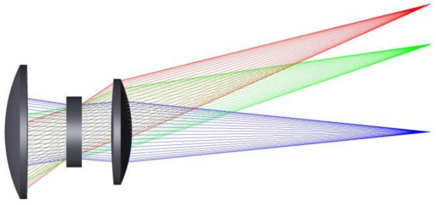
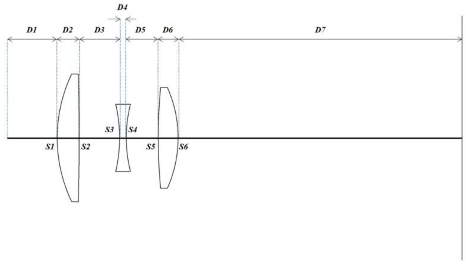
In this paper, a Cooke triplet lens is implemented for the optimization problem. Even with only three lenses, the optimization problem related to the curvature of surfaces, thickness of element and airspace, and selection of element glass is not trivial. Moreover, optimization of the triplet offers constructive insight concerning the characteristics of appropriate optimization algorithms.

1.2. Overview of Surrogate-Based Modelling

A surrogate model is also referred to as a “metamodel”, “response surface model”, “approximation model”, or “emulator” in different research fields. In complex computer simulations, finding more data requires additional experiments, which would result in extensive material or economic cost as well as computational expense. Consequently, obtaining an analytical form of derivatives or the objective function is relatively challenging. However, the derivation of the information from a surrogate model is comparatively easier, as the analytical form is known and, hence, is cheaper to evaluate. Building through the sampled data that are obtained by evaluating a set of sample points in the target space via expensive analysis code, a surrogate model can be used to efficiently predict the output of the code at any unknown point [56].

The representative surrogate models include the polynomial response surface model (PRSM) [57,58], Kriging [59,60], radial basis functions (RBFs) [61,62], artificial neural network (ANN) [63,64], support vector regression (SVR) [65,66], etc.

According to Anthony et al. [67] and Balabanov and Haftka [68], PRSM can be applied in aircraft design. Kriging is based on the idea that a surrogate can be represented as a realization of a stochastic process. This idea was first proposed in the field of geostatistics by Krige [69] and Matheron [70]. It gained popularity after being used for the design and analysis of computer experiments by Sacks, Welch, Mitchell, and Wynn [60]. Kriging is also known as a Gaussian process regression in the field of machine learning [71,72]. Kriging is used for process flowsheet simulations [73], design simulations [74], pharmaceutical process simulations [75], and feasibility analysis [76]. Radial basis functions have been developed for the interpolation of scattered multivariate data. RBFs are used for feasibility analysis [77] and parameter estimation [78]. ANN is used for process modelling [79], process control [80], and optimization [81,82]. SVR is shown to achieve comparable accuracy with that of other surrogates [83]. SVR models are accurate as well as fast in prediction; however, the time required to build this model is high because finding the unknown parameters requires solving a quadratic programming problem. This added complexity hinders the popularity of SVR [6].

Among them, Kriging has earned popularity in the fields of aerodynamic design optimization [84,85,86,87,88] and structural and multidisciplinary optimization [89,90]. Generally, geostatistical interpolation methods that calculate the spatial autocorrelation between measurements and utilize the spatial structure of measurements around the prediction location comprise universal Kriging, ordinary Kriging, and co-Kriging [91]. Isotropy (uniform values in all directions) is assumed during the Kriging process unless anisotropy is specified. Consequently, comparisons between isotropic and anisotropic semi-variogram-derived surfaces are not often made. Thus far, the application of anisotropy within Kriging has been shown to be superfluous for local- and regional-scale modelling, although Luo et al. [90] hypothesized that it may be more useful for meso- and macro-scale modelling.

According to the properties of surrogate-based models, Kriging is quite suitable for the multi-objective optimization of optical systems with high dimensions; hence, in this paper, the surrogate-based model applied to the triplet is Kriging.

1.3. Design of Experiments (DOE)

Defined as a process for choosing a series of sample points in the design space and with a general target of gaining maximum information from a constrained set of samples, design of experiments (DOE) can be divided into two categories: classical and modern techniques. The classical DOE originated from the random error that exists in a non-repeatable laboratory experiment (e.g., experimental chemistry and agricultural yield studies), while modern DOE, which includes the deterministic computer simulations, can eliminate the influence of non-repeatability. Therefore, to provide a more convincing result with non-repeatable experiments, classical DOE approaches mainly involve designs of fractional-factorial [92,93], full-factorial [94], Box–Behnken [95], and central composite [96], which normally locate sample points at the boundaries of the target space. In order to obtain the tendency of information accurately, modern DOE primarily employs space-filling designs, and the approaches in modern DOE mainly include Latin hypercube sampling (LHS) [97,98], pseudo-Monte Carlo sampling [99], quasi-Monte Carlo sampling [100], and orthogonal array sampling [101].

Modern DOE is also distinguished from classical DOE in the aspect of choosing the probability distribution functions of design parameters. In modern DOE, the probability of design parameters can be distributed uniformly and non-uniformly (e.g., Gaussian, Weibull); on the contrary, the possible values of a design parameter in classical DOE are typically assumed to be distributed uniformly between the lower and upper extremes. Additionally, the data generated in the design and analysis of computer experiments (DACE) [6,102,103,104,105] study of an optical imaging system can be applied in surrogate functions, normally expressed as response surface approximations [106], to assist the optimization process. Considering the complex relationships among input design parameters and imaging quality in the design of optical imaging systems, the independent sample points in the design and analysis of computer experiments (DACE) make it possible to utilize parallel computing, either on a multiprocessor computer or over a network [107].

Providentially, a perennial study in mathematical formulation leveraged by the progress in computer power enabled techniques developed for DACE to be successfully employed in various problems (e.g., design of energy and aerospace [108,109,110] systems, manufacturing [111], bioengineering [112,113], and decision under uncertainty [114]). Such techniques comprise a series of methodologies for generating a surrogate model, which can be used to substitute the expensive simulation code. The aim is to build an estimate of the response that is as accurate as possible under a limited number of expensive simulations [115].

Among the modern DOE methods, Metropolis and Ulam [99] first applied pseudo-Monte Carlo sampling into the field of computer simulations in 1949, with the utilization of a pseudo-random number generation algorithm aimed to imitate an indeed random natural procedure. Pseudo-Monte Carlo sampling, also known as Monte Carlo (MC) sampling, is suitable for convex but not rectangular design spaces, whereas the employment in high-dimensional and non-convex design spaces is rather difficult.

Quasi-Monte Carlo sampling [100], also named low-discrepancy sampling, has a common characteristic with pseudo-Monte Carlo sampling in that both approaches were developed for multidimensional integration. One of the fundamental differences between them is that quasi-Monte Carlo sampling can almost generate uniform samplings in a high-dimensional space with the employment of a deterministic algorithm [116]. Stemming from MC sampling, the stratified Monte Carlo sampling method [117] can create a more uniform sampling and offer superior overall coverage of the design space.

Developed by McKay et al. [118] as a substitute for pseudo-Monte Carlo sampling, Latin hypercube sampling (LHS) is one of the most widely and prevalently used space-filling methods for DOE. Under certain assumptions associated with the function to be sampled, Latin hypercube sampling provides a more accurate estimate of the mean value of the function than does MC sampling. As a result, the LHS can estimate less error in the mean value than the mean value estimated with MC sampling, under the condition of an equal number of samples. Another attractive aspect of the Latin hypercube design is that it allows the user to tailor the number of samples to the available computational budget. That is, a Latin hypercube design can be configured with any number of samples and is not restricted to sample sizes that are specific multiples or powers of n.

However, with a considerable number of design variables, it is challenging for the Latin hypercube design to provide a good coverage of the entire high-dimensional design space. In order to break this curse of dimensionality, constructing space-filling designs in low-dimensional projections is a promising approach. Such approaches comprise randomized orthogonal arrays [117], orthogonal array-based Latin hypercube designs [118], and the construction of orthogonal Latin hypercube designs [119]. The introduction of orthogonality into the Latin hypercube design is directly beneficial in fitting data with polynomial models. In addition, orthogonality can be considered as a stepping-stone to designs that are space-filling in low-dimensional projections [120].

Latin hypercube designs [98,121] have become particularly popular among all strategies mentioned above for computer experiments. According to Viana [115], the Latin hypercube design has a close growth rate in publications with DACE. Further evidence of the popularity of the Latin hypercube design is the number and diversity of the reported applications in which the LHS is used. 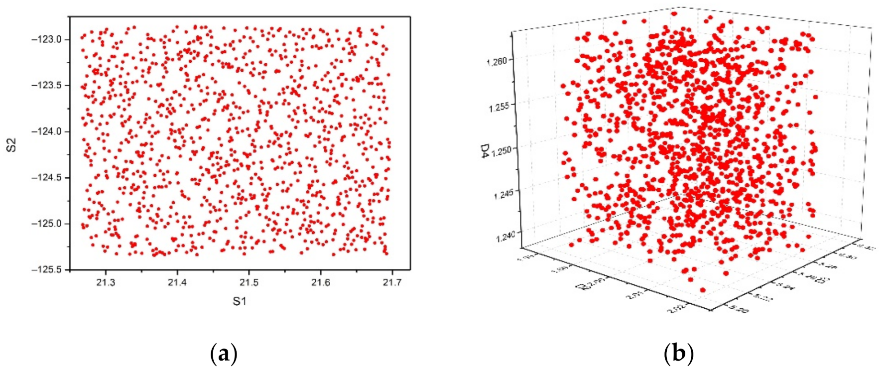For example, with the dedication of evaluating applications of surrogate modeling, the Latin hypercube design appears in eight out of the sixteen chapters in the book edited by Koziel and Leifsson [122]. On account of the advantages and popularity of the Latin hypercube design, it was chosen as the DACE method in this paper.

1.4. Multi-Objective Optimization (MOO)

In practical engineering, problems encountered by engineers with multiple objectives are known as multi-objective problems (MOPs), and MOPs with at least four objectives are casually known as many-objective problems (MaOPs) [123]. Multi-objective evolutionary algorithms (MOEAs) are typically applied to solve MOPs, which can be divided into decomposition-based [123,124,125,126], indicator-based [127,128], and Pareto-based [129,130,131] algorithms. However, it should be pointed out that the MOEAs confront three challenges when handling MaOPs, namely, dominance resistance (DR) phenomenon, dimensional curse, and visualization difficulty [132]. To solve the first challenge efficiently, three methods have been introduced, including modification of the Pareto dominance relation, an indicator-based approach, and enhanced diversity management [133].

Even though these methods can deal with MOPs effectively, there are still high computational burdens. The third approach for MaOPs is to enhance diversity management. For example, the NSGA-II [134] algorithm managed the activation and deactivation of the crowding distance to maintain diversity. As one of the Pareto-based algorithms, NSGA-III [135,136] achieved great success in practical application, which replaced the crowding distance operator in the NSGA-II with a clustering operator and used a set of well-distributed reference points to guarantee diversity. Although the NSGA-III algorithm can achieve good diversity, its performance needs to be improved by remedying deficiency or expanding application.

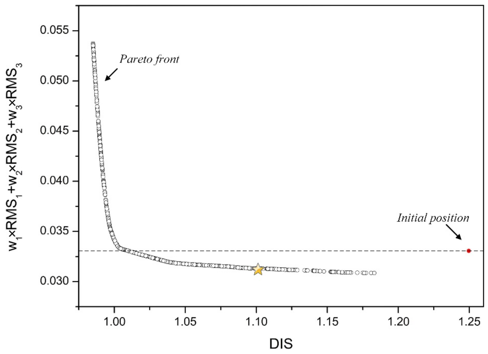
In this paper, the multi-objective algorithm NSGA-III is adopted in the model proposed. NSGA-III has been widely applied to different areas, such as the economic dispatch problem [137] and the ship hull form optimization [138]. This algorithm does not need to convert multiple targets into a single one. It can directly optimize multiple targets at the same time and provide a non-dominated solution set as output. From this solution set, designers can search for the optimal solutions according to their optimization focus and strategy. The multi-objective optimization method proposed in this paper has great potential to be used in the design process of complex high-precision optical systems [15,135,136].

2. Methodology

Compared with the above-mentioned methods/models, the surrogate model-based multi-objective optimization method presented in this paper is a data-driven method. It trains the surrogate model using a relatively small set of sample data before optimizing the design. Sample points are chosen using the DOE algorithms, and the data set can then be obtained by simulation at sample points using optical tracking methods, such as ray tracing. Benefiting from the surrogate model, this method has a low calculation cost. This is especially useful when the amount of calculation is very high, such as for the optimization of multiple objectives in a design space with high dimensionality.

2.1. Process Flow

Figure 1 shows the specific process steps of the method proposed in this paper, including:

• Decide on design parameters, including their ranges: the key design parameters that affect the performance of the optical system need to be decided first.
• Experimental design: based on the number and range of parameters given in step 1, DOE needs to be carried out to decide the sample points in the design space and provide information including the number of samples and their distribution.
• Sample points calculation: the ray-tracing-based program is then used to complete the calculation at each sample point and provide the interested targets required in the optimization.
• Surrogate model training: the surrogate model can be trained using the output from the sample points in step 3. The accuracy of the trained model is estimated, and more sample points are required if the accuracy cannot meet the requirements.
• Multi-objective optimization design: the multi-objective optimization algorithm is used at this step to optimize the design based on the prediction of the surrogate model and provide the final Pareto solution set as output.
• Decision making: the final optimal design can then be chosen from the Pareto solution set depending on the desired design focus and strategy.

2.2. DOE Method

For optical imaging system design, the relationships among input design parameters and imaging quality are very complex. It would be prohibitively time-consuming to perform all the possible computer experiments in order to comprehend these relationships or find the optimal design. The statistical design of experiments is a technique that can be used to design a limited number of samples that could reflect the design space information.

For the conventional optical imaging system, the number of design parameters is in the range of 10¹ to 10². Among the experimental design methods for computer experiments discussed in Section 1.3, the Latin hypercube design was applied in this model. As a modern and popular method for space-filling experimental design, LHS is a type of stratified Monte Carlo (MC), which allows the experimental designer total freedom in selecting the number of designs to run (as long as it is greater than the number of parameters). The Latin hypercube design is suitable for computer experiments with considerably large dimensions of the design space and has the advantage that the number of samples is not limited by the number of design parameters. Its operation process is simple and flexible and meets the requirement of reducing the sample scale in the case of a large number of design parameters. At present, the Latin hypercube design has become particularly popular among strategies for computer experiments [98].

In view of the above-mentioned advantages, LHS was chosen as the DOE algorithm for the computer experiment of the optical imaging system. The Latin hypercube design requires the designer to specify the number of parameters and their ranges, as well as the number of sample points to run. Assuming that the dimension of the design space is n, the number of sample points to be extracted is $ns$, and the value range in a certain dimension is $x\in \left[l_i,u_i\right]\left(i=1,2,\dots ,n\right)$, where, $l_i$ is the lower limit for the i-th parameter, and $u_i$ is the upper limit for the i-th parameter. The main steps of the LHS experimental design are as follows:

• Give the scale of sampling $ns$.
• Divide the value range $\left[l_i,u_i\right]$ of each dimension parameter $x_i$ into $ns$ intervals equally, then the design space can be divided into $ns\times n$ sub-areas.
• Randomly generate a matrix $X$ with the order of $ns\times n$. Each column of this matrix is a random arrangement from 1 to $ns$ (elements are $X_{i,j}, i=1\cdots ns,j=1\cdots n$, which are random integers in the range from 1 to $ns$). The matrix $X$ is called a Latin hypercube.
• Each row of the matrix $X$ corresponds to a selected small hypercube, which is a sample point. The normalized value of the i-th sample point for the j-th parameter can be calculated as:$x_{i,j}=\left(X_{i,j}-0.5\right)/ns$.

The actual value of the parameter for each sample point can be obtained by mapping $x_{i,j}$ into the design space considering the actual range.

Figure 2 shows the results of extracting 200 sample points in a two-dimensional space (each dimension range is [0, 1]) and 500 sample points in a three-dimensional space (each dimension range is [0, 1]) using the LHS method. The LHS method can guarantee that the number of projections of samples in each dimension of the design parameters is equal to the number of samples, and the projections have uniform distribution in each dimension.

2.3. Kriging Surrogate Model

The Kriging surrogate model originated in the areas of mining and geostatistics, which involve temporally and spatially correlated data. The unique characteristic of Kriging stems from its ability to combine global and local modeling. The Kriging surrogate model is one of the unbiased models with the smallest estimation variance, which could provide efficient and reliable prediction. Extensive reviews of the Kriging model used in simulation, sensitivity analysis, and optimization in the design process can be found in [139]. Due to its high accuracy and good performance for complex nonlinear problems, the Kriging surrogate model was chosen as the surrogate model to provide prediction for the imaging quality of the optical imaging system in this paper.

The Kriging model consists of two parts, the regression model and the stochastic process. The regression model represents the global tendency of the analyzed function, and the stochastic process represents the spatial correlations in the design space of interest [140].

$$y=\underset{i=1}{\overset{k}{\Sigma }}{\beta }_i{f}_i\left(x\right)+Z\left(x\right)$$

(1)

where x is n-dimensional vector,$y$is the unknown function of ${\beta }_i{f}_i$ (regression model) and Z(x) (stochastic process).

The regression models with polynomials of orders 0, 1 and 2 were adopted here and detailed in

Table 1. Regression models.

Orders	Number k	Function fi
0 (constant)	k = 1	$f_1\left(x\right)=1$
1 (linear)	k = n + 1	$f_1\left(x\right)=1$$, f_2\left(x\right)=x_1$$, \dots , f_{n+1}\left(x\right)=x_n$
2 (quadratic)	k = (n + 1)(n + 2)/2	$f_1\left(x\right)=1$$, f_2\left(x\right)=x_1$$, \dots , f_{n+1}\left(x\right)=x_n$ $f_m\left(x\right)=x_i{x}_j i=1,\dots ,n, j=1,\dots ,n$

.

Z(x) represents a local deviation from the regression model and is the realization of a stationary, normally distributed Gauss random process with zero mean, variance, and non-zero covariance. The covariance matrix of Z(x) is given by:

$$cov\left[Z\left(x^{\left(i\right)}\right),Z\left(x^{\left(j\right)}\right)\right]={\sigma }^{2}R\left(x^{\left(i\right)},x^{\left(j\right)}\right) i,j=1,\dots ,ns$$

(2)

where ${\sigma }^2$ is the process variance, and $R$ is an ns × ns symmetric correlation matrix. In addition, $\mathrm{R}\left(x^{\left(i\right)},x^{\left(j\right)}\right)$ is the spatial correlation function between any two points$x^{\left(i\right)}$ and $x^{\left(j\right)}$ of ns sample points. A popular Gaussian correlation function is used here, and the function can be expressed:

$$R\left(x^{\left(i\right)},x^{\left(j\right)}\right)=\exp \left[-{\displaystyle \sum }_{k=1}^m{\theta }_k{\left|x^{\left(i\right)}-x^{\left(j\right)}\right|}^2\right]$$

(3)

where θ_k is the k_th element of the correlation vector parameter θ. The regression term ${{\displaystyle \sum }}_{i=1}^k{\beta }_i{f}_i\left(x\right)$ can choose a constant value, a linear model, or a quadratic model. In this paper, the quadratic model was adopted here. In the implementations, x is normalized by subtracting the mean from each variable, and then dividing the values of each variable by its standard deviation:

$$x_{\mathrm{norm} }=\frac{x-x_{\mathrm{mean} }}{x_{\mathrm{std} }}$$

(4)

The Kriging predictor is:

$$\widehat{y}\left(x\right)=\widehat{\mu }+r{\left(x\right)}^T{R}^{-1}\left(Y-F\widehat{\mu }\right)$$

(5)

where $F$ is a matrix that can be written as:

$$F=\left[\begin{array}{ccc}{f}_1\left({\mathit{x}}_1\right)& \cdots & f_k\left({\mathit{x}}_1\right)\\ ⋮& \ddots & ⋮\\ f_1\left({\mathit{x}}_{ns}\right)& \cdots & f_k\left({\mathit{x}}_{ns}\right)\end{array}\right]$$

When the order of the regression models is 0, F is a column vector of length ns filled with ones. Y the column vector with responses of sample points, and r(x) is the correlation vector, which can be written as:

$$r\left(x\right)={\left[R\left(x,x^1\right),R\left(x,x^2\right),I,R\left(x,x^{n_s}\right)\right]}^T$$

(6)

For a give parameter θ, $\widehat{\mu }$ and ${\widehat{\sigma }}^2$ can be calculated as:

$$\widehat{\mu }={\left(F^T{R}^{-1}F\right)}^{-1}{F}^T{R}^{-1}Y$$

(7)

$$\widehat{\sigma }{ }^2=\frac{1}{n_s}{\left(Y-F\widehat{\mu }\right)}^T{R}^{-1}\left(Y-F\widehat{\mu }\right)$$

(8)

The uncertainty of the predicted value of the Kriging model can be expressed as:

$$s^2\left(x\right)=\widehat{\sigma }{ }^2\left(1-r^T{R}^{-1}r+\frac{{\left(1-F{R}^{-1}r\right)}^2}{F^T{R}^{-1}F}\right)$$

(9)

Due to $\widehat{\mu }$, ${\widehat{\sigma }}^2$, r(x), and correlation matrix R being dependent on the parameter θ, the Kriging model is trained by finding a parameter θ that maximizes the following likelihood function. Unlike the deep neural networks, the goodness-of-fit of the Kriging model is not clearly defined. For the Kriging model, the value of $ln\left(Likelihood\right)$has a similar effect to the goodness-of-fit. A larger value of $ln\left(Likelihood\right)$ represents a better-fitting effect of the Kriging model.

$$ln\left(Likelihood\right)=\frac{1}{2}\left(nln\widehat{\sigma }{ }^2+ln\left|R\right|\right)$$

(10)

The process to find a parameter $\theta$ that maximizes the likelihood function is to solve an unconstrained optimization problem. For the Kriging model in the present paper, optimization algorithms such as the Genetic Algorithm (GA) [141], Particle Swarm Optimization (PSO) [142], and the pattern search algorithm [143] are used for this purpose. The GA and the PSO was chosen when the dimension was lower than 10 [144].

To verify the reliability of the surrogate model, it is important to test the model using test sample points, based on different error evaluation criteria, such as the average relative error, root-mean-square error, and correlation coefficient. The definition formula of these criteria are as follows:

$$ARE=\frac{1}{N}{\displaystyle \sum }_{i=1}^N\left(\frac{f_i\left(x\right)-\widehat{f_i}\left(x\right)}{f_i\left(x\right)}\right)$$

(11)

$$RMSE=\frac{\sqrt{\frac{1}{N}{{\displaystyle \sum }}_{i=1}^N{\left(f_i\left(x\right)-\widehat{f_i}\left(x\right)\right)}^2}}{\frac{1}{N}{{\displaystyle \sum }}_{i=1}^N\left|f_i\left(x\right)\right|}$$

(12)

$$Correlation Coefficient=\frac{{{\displaystyle \sum }}_{i=1}^N\left(f_i\left(x\right)-\overline{f_i\left(x\right)}\right)\left(\widehat{f_i}\left(x\right)-\overline{\widehat{f_i}\left(x\right)}\right)}{\sqrt{{{\displaystyle \sum }}_1^N{\left(f_i\left(x\right)-\overline{f_i\left(x\right)}\right)}^2}\sqrt{{{\displaystyle \sum }}_1^N{\left(\widehat{f_i}\left(x\right)-\overline{\widehat{f_i}\left(x\right)}\right)}^2}}$$

(13)

2.4. NSGA-III Multi-Objective Optimization Algorithm

Most multi-objective optimization algorithms using evolutionary optimization methods have demonstrated their efficiency in various practical problems involving mostly two and three objectives. There is a growing need for developing multi-objective optimization algorithms for handling optimization problems with more objectives. The multi-objective optimization algorithm used in this paper is the Non-dominated Sorting Genetic Algorithm III (NSGA-III) [136], which is an upgrade from NSGA-II [134]. NSGA-III is a reference-point-based many-objective evolutionary algorithm that emphasizes population members that are non-dominated, yet close to a set of supplied reference points.

The framework of NSGA-III is basically the same as that of NSGA-II. The biggest change in NSGA-III is the use of the well-distributed reference points to maintain a good diversity of the population. Therefore, it shows a better diversity and convergence. It also uses the simulated binary crossover (SBX) [145], mutation operator (polynomial mutation), and Pareto sorting in the process and selects population in the key layer L, using a niching algorithm rather than the crowding distance method used in NSGA-II. In order to deal with the constraint problem, the model used here also adopted the penalty method, which means a certain penalty value would be added to the individual for triggering the constraint depending on its adaptability.

The steps of using the NSGA-III algorithm are as follows:

• Generate the initial population$P_o$, which contains N randomly generated individuals.
• Conduct binary competition selection, simulated binary crossover, and mutation operations on individuals in the initial population to generate $N$ offspring populations $Q_o$.
• Merge the parent and child populations. The number of individuals in the new population is $2N$.
• Apply a fast non-dominated sorting technique on the population to obtain the individuals’ order and carry on selecting the next generation population $P1$.
• Decide whether the conditions have been reached for terminating the iteration. If it is, output the individuals; otherwise, go to step 2.

3. Case Studies of a Cooke Triplet System

Two case studies focusing on a Cooke triplet optical system were carried out using the method introduced in Section 2. In the first case, the optimization was carried out on a classic Cooke triplet system simply to prove that the model proposed can be applied to an optical system. The second case starts the optimization from a system that has been optimized using a commercial software, CODE-V (version: codev 10.8) [146], in order to show that the model can further improve the results.

3.1. Case 1

A Cooke triplet system that consists of three lenses was used as the optimization design subject, as shown in Figure 3. The geometric shape and the distance between the lens were selected as the design parameters. The optimization’s objectives were to minimize the maximum field curvature (DIS) and the geometric spot diagram (RMS) of the Cooke triplet system. The front and back curvature, thickness, and spacing of each lens were chosen as the design parameters. In total, there were 12 of them (not including D1, which is the distance to the system’s origin), as shown in Figure 4. The initial design parameters from which the optimization started are listed in

Table 2. Initial design parameters of Cooke triplet (Case 1).

Parameter	(Unit: mm)
S1	21.48138
S2	−124.1
S3	−19.1
S4	22
S5	328.9
S6	−16.7
D2	2
D3	5.26
D4	1.25
D5	4.69
D6	2.25
D7	43.0504842168944

.

Since there are two objectives, minimizing DIS and RMS, this was a two-objective optimization. Here, DIS was treated as a single value, while the three RMS were combined into one by using weighting factors, as seen in Equations (14) and (15). The weighting factors w₁, w₂, and w₃ used here were 0.3, 0.35, and 0.35, respectively.

$$Aim1: min\left(DIS\right)$$

(14)

$$Aim2: min (w_1\times RM{S}_1+w_2\times RM{S}_2+w_3\times RM{S}_3)$$

(15)

The range of variation for each design parameter was set as ±1% of the initial value. The LHS method was used to choose 1200 sample points within this 12-dimension design space.

Figure 5 shows the projections of these sample points in a 2D space (S1 X S2) and a 3D space (D2 X D3 X D4).

A commercial software, CODE-V [146], was used to carry out the calculation at these sample points using a ray-tracing-based method and to provide the DIS and RMS at these sample points. Of the sample results, 95% were randomly selected as the training data for the Kriging surrogate model, and the remaining 5% were used for testing.

Table 3. Evaluation results of the trained surrogate model.

Evaluation Parameter	DIS	RMS1	RMS2	RMS3
Average Relative Error	3.18682 × 10−6	0.0513925	0.00582908	0.006664
Root-Mean-Square Error	5.49953 × 10−6	0.00098156	0.000428076	0.0003938
Correlation Coefficient	1.00	0.99578	0.999379	0.998721

shows the evaluation results of each target value based on the 5% testing samples. From the table, the Correlation Coefficients are all close to 1. The Relative Errors are less than 1% except RMS1, which is 5%.

Multi-objective optimization was conducted using the NSGA-III algorithm. The population number was set at 1000, and the evolutionary generation was set at 2000. Figure 6 shows the Pareto frontier at different evolution steps in the evolution process. The shape of the frontier tends to stabilize after about 100 generations (last is 2000).

The final Pareto frontier solution set and the initial design are shown in the Figure 7. Since this was a multi-objective analysis, the final result was not unique but a set of non-dominated solutions. It is very obvious that the optimization process significantly reduced both the weighted RMS and DIS. The final optimal solution can be chosen from the solution set depending on the design focus and strategy.

For example, the strategy here was to minimize the weighted RMS providing the DIS an acceptable level. Here, the level was set at 1.10. One final solution, shown as a blue star in Figure 7, can then be chosen from the solution set.

A comparison of the DIS and RMS before and after the optimization is shown in

Table 4. Comparison of results before and after optimization.

Physical Quantity	Before Optimization (CODE V)	Optimization Result
DIS	1.24963	1.104833510
w1 × RMS1 + w2 × RMS2 + w3 × RMS3	0.03306	0.031301775
RMS1	0.00856	0.009467504
RMS2	0.04649	0.043443469
RMS3	0.04062	0.037875171

. The optimized solution reduced RMS by 5.32% and DIS by 11.59%. It significantly improved the performance of the Cooke triplet from its original design. The values of the 12 design parameters before and after the optimization are listed in

Table 5. Comparison of design parameters before and after optimization (Case 1).

Parameter	Initial Value (Unit: mm)	Optimized Value (Unit: mm)
S1	21.48138	21.65449
S2	−124.1	−124.40895
S3	−19.1	−19.28859
S4	22	22.14426
S5	328.9	325.61100
S6	−16.7	−16.74972
D2	2	2.01141
D3	5.26	5.20719
D4	1.25	1.25230
D5	4.69	4.73700
D6	2.25	2.25106
D7	43.0504842168944	42.95710

.

Since the optimized solution was obtained from the Kriging surrogate model, not from an actual calculation, it was put into CODE-V for an actual calculation as a double check. The results are shown in

Table 6. Checking optimization results.

Physical Quantity	Optimized Value	CODE V Check	Deviation (%)
DIS	1.104833510	1.10483	−0.000318%
w1 × RMS1 + w2 × RMS2 + w3 × RMS3	0.031301775	0.031167	−0.429832%
RMS1	0.009467504	0.009824	3.761249%
RMS2	0.043443469	0.04291	−1.227962%
RMS3	0.037875171	0.037719	−0.412330%

. The deviation for DIS and weighted RMS between the optimized solution and the CODE-V calculation is less than 0.5%. The maximum deviation for an individual RMS is 3.7%.

3.2. Case 2

Since CODE V has its own built-in optimization module and it has been used as an industrial standard, a case study was carried out to show that the model presented here can further improve the CODE-V’s optimization result. The CODE-V optimized values are shown in

Table 7. Initial design parameters of Cooke triplet (Case 2).

Parameter	Value (Unit: mm)
S1	18.9211
S2	−55.9799
S3	−17.2447
S4	18.3846
S5	−105.9429
S6	−15.2416
D2	2
D3	4.5035
D4	1.25
D5	6.675
D6	2.25
D7	41.5769

and

Table 8. DIS and RMS values of optimized objects.

Physical Quantity	Value
DIS	0.65474
RMS1	0.005349
RMS2	0.010732
RMS3	0.010352

. These were used as the starting point of the optimization process in Case 2.

The other settings were all the same as Case 1. Based on the prediction of the Kriging surrogate model for the testing data, the Correlation Coefficient of the prediction results were all greater than 0.971, and the Relative Errors were less than 3% except RMS1, which was 5.6%.

Multi-objective optimization was conducted using the NSGA-III algorithm, with the setting of 1000 population and 2000 evolutionary generations. Figure 8 shows the final Pareto frontier solution set with the initial state.

As seen from Figure 8, although CODE-V has optimized its output, the model presented here can still further improve the optimization design. If the DIS value is chosen as 0.63 as an acceptable value, the final optimization solution can be obtained from the solution set. The design parameters and targeted values before and after the optimization are listed in

Table 9. Comparison of design parameters before and after optimization (Case 2).

Parameter	Initial Value (Unit: mm)	Optimized Value (Unit: mm)
S1	18.9211	19.051388
S2	−55.9799	−55.586519
S3	−17.2447	−17.268053
S4	18.3846	18.303013
S5	−105.9429	−105.810608
S6	−15.2416	−15.151970
D2	2	1.996235
D3	4.5035	4.469327
D4	1.25	1.254227
D5	6.675	6.649926
D6	2.25	2.252321
D7	41.5769	41.567974

and

Table 10. Comparison of key parameters before and after optimization.

Physical Quantity	Before Optimization	After Optimization
DIS	0.65474	0.6264
w1 × RMS1 + w2 × RMS2 + w3 × RMS3	0.008984	0.008667
RMS1	0.005349	0.0048218
RMS2	0.010732	0.0091484
RMS3	0.010352	0.011481

.

The optimized solution further improved the performance of the Cooke triplet, with a 3.53% reduction in weighted RMS and a 4.33% reduction in the DIS.

4. Conclusions

An optimization model based on a surrogate model and a multi-objective optimization algorithm for an optical imaging system was established in this paper. The use of a surrogate model can significantly reduce the calculation cost but still keep a high level of accuracy, especially when the design space has a large dimension. Another advantage of this model is the ability to optimize multiple objectives simultaneously during the optimization process. This is achieved by using a multi-objective optimization algorithm. With the surrogate model and the multi-objective optimization algorithm, this model can significantly improve the efficiency of optical design.

Two case studies of optimizing a Cooke triplet optical system were carried out with twelve design parameters and two optimization objectives:

Case 1 showed that the optimized result from the model significantly improved the imaging quality of the initial design, with a reduction of 5.32% in RMS and 11.59% in DIS. Further verification conducted using CODE-V showed that the deviation from an actual calculation was less than 0.5%.

Case 2 used an optimized result from CODE-V as the starting point and showed that the optimization from the model presented further reduced the weighted RMS by 3.53% and the DIS by 4.33%.

As a result, the model presented in this paper is suitable for the optimization of optical system design, and it can further improve the optimization results from CODE-V. It has great potential to be used in the design process of complex high-precision optical systems.

References

1. Jamieson, T.H. Optimization Techniques in Lens Design; A. Hilger: London, UK, 1971. [Google Scholar]
2. Dilworth, D.C. Automatic Lens Optimization: Recent Improvements. SPIE 1986, 554, 191–196. [Google Scholar]
3. Ernest, B.R. [Dynamic Programming]; Dover Publications Inc.: New York, NY, USA, 2003. [Google Scholar]
4. Hegde, R.S. Accelerating optics design optimizations with deep learning. Opt. Eng. 2019, 58, 065103. [Google Scholar] [CrossRef]
5. Queipo, N.V.; Haftka, R.T.; Shyy, W.; Goel, T.; Vaidyanathan, R.; Tucker, P.K. Surrogate-based analysis and optimization. Prog. Aerosp. Sci. 2005, 41, 1–28. [Google Scholar] [CrossRef] [Green Version]
6. Forrester, A.; Keane, A.J. Recent advances in surrogate-based optimization. Prog. Aerosp. Sci. 2009, 45, 50–79. [Google Scholar] [CrossRef]
7. Liu, D.; Tan, Y.; Khoram, E.; Tan, Y.; Khoram, E.; Yu, Z. Training Deep Neural Networks for the Inverse Design of Nanophotonic Structures. Am. Chem. Soc. 2018, 5, 1365–1369. [Google Scholar] [CrossRef]
8. Liu, Z.; Zhu, D.; Rodrigues, S.P.; Lee, K.-T.; Cai, W. Generative Model for the Inverse Design of Metasurfaces. Nano Lett. 2018, 18, 6570–6576. [Google Scholar] [CrossRef] [Green Version]
9. Zhang, T.; Wang, J.; Liu, Q.; Zhou, J.; Dai, J.; Han, X.; Zhou, Y.; Xu, K. Efficient Spectrum Prediction and Inverse Design for Plasmonic Waveguide System Based on Artificial Neural Networks. Photonics Res. 2018, 7, 368–380. [Google Scholar] [CrossRef] [Green Version]
10. Malkiel, I.; Michael, M.; Nagler, A.; Arieli, U.; Wolf, L.; Suchowski, H. Plasmonic nanostructure design and characterization via Deep Learning. Light Sci. Appl. 2018, 7, 60. [Google Scholar] [CrossRef]
11. Wiecha, P.R.; Lecestre, A.; Mallet, N.; Larrieu, G. Pushing the limits of optical information storage using deep learning. Nat. Nanotechnol. 2019, 14, 237–244. [Google Scholar] [CrossRef]
12. Kan, Y.; Unni, R.; Zheng, Y. Intelligent Nanophotonics: Merging Photonics and Artificial Intelligence at the Nanoscale. Nanophotonics 2018, 8, 339–366. [Google Scholar]
13. Wei, M.; Cheng, F.; Liu, Y. Deep-Learning-Enabled On-Demand Design of Chiral Metamaterials. ACS Nano 2018, 12, 6326–6334. [Google Scholar]
14. Inampudi, S.; Mosallaei, H. Neural network based design of metagratings. Appl. Phys. Lett. 2018, 112, 241102. [Google Scholar] [CrossRef]
15. Garrido-Merchán, E.C.; Hernández-Lobato, D. Dealing with categorical and integer-valued variables in Bayesian Optimization with Gaussian processes. Neurocomputing 2020, 380, 20–35. [Google Scholar] [CrossRef] [Green Version]
16. Kleijnen, J. Kriging metamodeling in simulation: A review. Eur. J. Oper. Res. 2009, 192, 707–716. [Google Scholar] [CrossRef] [Green Version]
17. Audet, C.; Denni, J.; Moore, D.; Booker, A.; Frank, P. A Surrogate-Model-Based Method for Constrained Optimization. In Proceedings of the AIAA/USAF/NASA/ASSMO Symposium on Multidisciplinary Analysis & Optimization, Long Beach, CA, USA, 6–8 September 2000. [Google Scholar]
18. Jeong, S.; Obayashi, S.; Yamamoto, K. Aerodynamic optimization design with Kriging model. Trans. Jpn. Soc. Aeronaut. Space Sci. 2005, 48, 161–168. [Google Scholar] [CrossRef]
19. Shtiliyanova, A.; Bellocchi, G.; Borras, D.; Eza, U.; Martin, R.; Carrère, P. Kriging-based approach to predict missing air temperature data. Comput. Electron. Agric. 2017, 142, 440–449. [Google Scholar] [CrossRef]
20. Zhang, W. An adaptive order response surface method for structural reliability analysis. Eng. Comput. 2019, 36, 1626–1655. [Google Scholar] [CrossRef]
21. Sahin, F.E. Open-Source Optimization Algorithms for Optical Design. Optik 2018, 178, 1016–1022. [Google Scholar] [CrossRef]
22. Feder, D.P. Automatic lens design methods. J. Opt. Soc. Am. 1957, 47, 902. [Google Scholar] [CrossRef]
23. Wynne, C.G. Lens Designing by Electronic Digital Computer: I. Proc. Phys. Soc. Lond. 1959, 73, 777. [Google Scholar] [CrossRef]
24. Juergens, R.C. The Sample Problem: A Comparative Study of Lens Design Programs and Users. J. Opt. Soc. Am. 1980, 70, 348–363. [Google Scholar]
25. Mcguire, J.P.; Kuper, T.G. Approaching direct optimization of as-built lens performance. Proc. SPIE-Int. Soc. Opt. Eng. 2012, 8487, 84870D. [Google Scholar]
26. Sahin, F.E. Lens design for active alignment of mobile phone cameras. Opt. Eng. 2017, 56, 065102. [Google Scholar] [CrossRef]
27. Heide, F.; Rouf, M.; Hullin, M.B.; Labitzke, B.; Heidrich, W.; Kolb, A. High-Quality Computational Imaging Through Simple Lenses. ACM Trans. Graph. 2013, 32, 149. [Google Scholar] [CrossRef]
28. Li, W.; Yin, X.; Liu, Y.; Zhang, M. Computational imaging through chromatic aberration corrected simple lenses. J. Mod. Opt. 2017, 64, 2211–2220. [Google Scholar] [CrossRef]
29. Sahin, F.E.; Tanguay, A.R. Distortion optimization for wide-angle computational cameras. Opt. Express 2018, 26, 5478–5487. [Google Scholar] [CrossRef]
30. Rosen, S.; Eldert, C. Least-Squares Method for Optical Correction. J. Opt. Soc. Am. 1954, 44, 250–251. [Google Scholar] [CrossRef]
31. Meiron, J. Damped Least-Squares Method for Automatic Lens Design. J. Opt. Soc. Am. 1965, 55, 1105–1109. [Google Scholar] [CrossRef]
32. Buchele, D.R. Damping Factor for the Least-Squares Method of Optical Design. Appl. Opt. 1968, 7, 2433–2435. [Google Scholar] [CrossRef]
33. Morrison, D.D. Optimization by least squares. SIAM J. Numer. Anal. 1968, 5, 83–88. [Google Scholar] [CrossRef]
34. Björck, Å. Least squares methods. Handb. Numer. Anal. 1990, 1, 465–652. [Google Scholar]
35. Berge, J. Least Squares Optimization in Multivariate Analysis; DSWO Press, Leiden University: Leiden, The Netherlands, 1993. [Google Scholar]
36. Kidger, M.J. The Application of Electronic Computers to the Design of Optical Systems, Including Aspheric Lenses. Ph.D. Thesis, University of London, London, UK, 1971. [Google Scholar]
37. Spencer, G.H. A Flexible Automatic Lens Correction Procedure. Appl. Opt. 1963, 2, 1257–1264. [Google Scholar] [CrossRef]
38. Grey, D.S. Aberration Theories for Semiautomatic Lens Design by Electronic Computers. I. Preliminary Remarks. J. Opt. Soc. Am. 1963, 53, 672–673. [Google Scholar] [CrossRef]
39. Grey, D.S. Aberration Theories for Semiautomatic Lens Design by Electronic Computers. II. A Specific Computer Program. J. Opt. Soc. Am. 1963, 53, 677–680. [Google Scholar] [CrossRef]
40. Pegis, R.J.; Grey, D.S.; Vogl, T.P.; Rigler, A.K. The generalized orthonormal optimization program and its applications. In Recent Advances in Optimization Techniques; Lavi, A., Vogl, T.P., Eds.; John Wiley & Sons, Inc.: New York, NY, USA, 1966. [Google Scholar]
41. Metropolis, N.; Rosenbluth, A.W.; Rosenbluth, M.N.; Teller, A.H.; Teller, E. Equation of state calculations by fast computing machines. J. Chem. Phys. 1953, 21, 1087–1092. [Google Scholar] [CrossRef] [Green Version]
42. Gelatt, M.P.; Vecchi, S.; Kirkpatrick, C.D. Optimization by Simulated Annealing. Science 1983, 220, 671–680. [Google Scholar]
43. Glatzel, E.; Wilson, R. Adaptive Automatic Correction in Optical Design. Appl. Opt. 1968, 7, 265–276. [Google Scholar] [CrossRef]
44. Rayces, J.L. Ten Years of Lens Design with Glatzel’s Adaptive Method. J. Opt. Soc. Am. 1980, 70, 75–84. [Google Scholar]
45. Darwin, C.R. The Origin of Species by Means of Natural Selection, or the Preservation of Favoured Races in the Struggle for Life; Books, Incorporated, Pub.: San Leandro, CA, USA, 1913. [Google Scholar]
46. Holland, J.H. Adaptation in Natural and Artificial Systems, 2nd ed.; MIT Press: Cambridge, MA, USA, 1992. [Google Scholar]
47. Jong, K.D. An Analysis of the Behaviore of a Class of Genetic Adaptive Systems. Ph.D. Thesis, University of Michigan, Ann Arbor, MI, USA, 1975. [Google Scholar]
48. Goldberg, D.E. Genetic Algorithms in Search, Optimization & Machine Learning; Addison-Wesley Publishing Co., Inc.: Reading, MA, USA, 1989. [Google Scholar]
49. Davis, L. Handbook of Genetic Algorithms; Van Nostrand Reinhold: New York, NY, USA, 1991. [Google Scholar]
50. Schwefell, H.P. Evolution and Optimum Seeking; John Wiley & Sons Inc.: New York, NY, USA, 1995. [Google Scholar]
51. Vasiljevi, D. Classical and Evolutionary Algorithms in the Optimization of Optical Systems; Springer Science & Business Media: Berlin/Heidelberg, Germany, 2012. [Google Scholar]
52. Yang, T.; Cheng, D.; Wang, Y. Direct generation of starting points for freeform off-axis three-mirror imaging system design using neural network based deep-learning. Opt. Express 2019, 27, 17228. [Google Scholar] [CrossRef]
53. Hegde, R. Deep neural network (DNN) surrogate models for the accelerated design of optical devices and systems. In Proceedings of the Novel Optical Systems, Methods, and Applications XXII, San Diego, CA, USA, 9 September 2019. [Google Scholar]
54. Peter, T. Using Deep Learning as a Surrogate Model in Multi-Objective Evolutionary Algorithms. Ph.D. Thesis, Otto-von-Guericke-Universität, Magdeburg, Germany, 2018. [Google Scholar]
55. Jin, Y. A comprehensive survey of fitness approximation in evolutionary computation. Soft Comput. 2005, 9, 3–12. [Google Scholar] [CrossRef] [Green Version]
56. Han, Z.H.; Zhang, Y.; Song, C.X.; Zhang, K.S. Weighted gradient-enhanced kriging for high-dimensional surrogate modeling and design optimization. AIAA J. 2017, 55, 4330–4346. [Google Scholar] [CrossRef] [Green Version]
57. Schmit, L.A.; Farshi, B. Some Approximation Concepts for Structural Synthesis. AIAA J. 1974, 12, 692–699. [Google Scholar] [CrossRef]
58. Box, G.E.P.; Drapper, N.R. Empirical Model Building and Response Surfaces. J. R. Stat. Soc. 1987, 30, 229–231. [Google Scholar]
59. Krige, D.G. A Statistical Approach to Some Basic Mine Valuation Problems on the Witwatersrand. J. Chem. Metall. Min. Soc. S. Afr. 1951, 94, 95–111. [Google Scholar]
60. Sacks, J.; Welch, W.J.; Mitchell, T.J.; Wynn, H.P. Design and Analysis of Computer Experiments. Stat. Sci. 1989, 4, 409–423. [Google Scholar] [CrossRef]
61. Powell, M.J.D. Algorithms for Approximation; Oxford University Press: New York, NY, USA, 1987. [Google Scholar]
62. Mullur, A.A.; Messac, A. Extended Radial Basis Functions: More Flexible and Effective Metamodeling. AIAA J. 2005, 43, 1306–1315. [Google Scholar] [CrossRef]
63. Park, J.; Sandberg, I.W. Universal Approximation Using RadialBasis-Function Networks. Neural Comput. 1991, 3, 246–257. [Google Scholar] [CrossRef]
64. Elanayar, S.V.T.; Shin, Y.C. Radial Basis Function Neural Network for Approximation and Estimation of Nonlinear Stochastic Dynamic Systems. IEEE Trans. Neural Netw. 1994, 5, 594–603. [Google Scholar] [CrossRef] [Green Version]
65. Smola, A.J.; Schölkopf, B.A. Tutorial on Support Vector Regression. Stat. Comput. 2004, 14, 199–222. [Google Scholar] [CrossRef] [Green Version]
66. Zhang, K.S.; Han, Z.H. Support Vector Regression-Based Multidisciplinary Design Optimization in Aircraft Conceptual Design. In Proceedings of the 51st AIAA Aerospace Sciences Meeting, Grapevine, TX, USA, 7–10 January 2013; AIAA Paper. p. 1160. [Google Scholar]
67. Anthony, A.G.; Vladimir, B.; Dan, H.; Bernard, G.; William, H.M.; Layne, T.W.; Raphael, T.H. Multidisciplinary Optimization of a Supersonic Transport Using Design of Experiments Theory and Response Surface Modeling; Virginia Polytechnic Institute & State University: Blacksburg, VA, USA, 1997. [Google Scholar]
68. Balabanov, V.; Haftka, R. Multifidelity response surface model for HSCT wing bending material weight. In Proceedings of the 7th AIAA/USAF/NASA/ISSMO Symposium on Multidisciplinary Analysis and Optimization, St. Louis, MO, USA, 2–4 September 1998; pp. 1–18. [Google Scholar]
69. Krige, D.G. A statistical approach to some mine valuation and allied problems on the Witwatersrand. J. S. Afr. Inst. Min. Metall. 1951, 52, 119–139. [Google Scholar]
70. Matheron, G. Principles of geostatistics. Econ. Geol. 1963, 58, 1246–1266. [Google Scholar] [CrossRef]
71. Rasmussen, C.E.; Williams, C. Gaussian Processes for Machine Learning; MIT Press: Cambridge, MA, USA, 2006. [Google Scholar]
72. Rasmussen, C.E.; Williams, C. Gaussian Processes for Machine Learning; MIT Press: Cambridge, MA, USA, 2005. [Google Scholar]
73. Palmer, K.; Realff, M. Metamodeling Approach to Optimization of Steady-State Flowsheet Simulations. Chem. Eng. Res. Des. 2002, 80, 760–772. [Google Scholar] [CrossRef]
74. Yang, R.J.; Wang, N.; Tho, C.H.; Bobineau, J.P.; Wang, B.P. Metamodeling Development for Vehicle Frontal Impact Simulation. J. Mech. Des. 2005, 127, 1014. [Google Scholar] [CrossRef]
75. Jia, Z.; Davis, E.; Muzzio, F.J.; Ierapetritou, M.G. Predictive modeling for pharmaceutical processes using kriging and response surface. J. Pharm. Innov. 2009, 4, 174–186. [Google Scholar] [CrossRef]
76. Rogers, A.; Ierapetritou, M. Feasibility and flexibility analysis of black-box processes part 2: Surrogate-based flexibility analysis. Chem. Eng. Sci. 2015, 137, 1005–1013. [Google Scholar] [CrossRef]
77. Wang, Z.; Ierapetritou, M. A novel feasibility analysis method for black-box processes using a radial basis function adaptive sampling approach. AIChE J. 2016, 63, 532–550. [Google Scholar] [CrossRef]
78. Müller, J.; Paudel, R.; Shoemaker, C.A.; Woodbury, J.; Wang, Y.; Mahowald, N. CH4 parameter estimation in CLM4.5bgc using surrogate global optimization. Geosci. Model Dev. 2015, 8, 3285–3310. [Google Scholar] [CrossRef] [Green Version]
79. Meert, K.; Rijckaert, M. Intelligent modelling in the chemical process industry with neural networks: A case study. Comput. Chem. Eng. 1998, 22, S587–S593. [Google Scholar] [CrossRef]
80. Mujtaba, I.M.; Aziz, N.; Hussain, M.A. Neural Network Based Modelling and Control in Batch Reactor. Chem. Eng. Res. Des. 2006, 84, 635–644. [Google Scholar] [CrossRef]
81. Fernandes, F.A.N. Optimization of fischer-tropsch synthesis using neural networks. Chem. Eng. Technol. 2006, 29, 449–453. [Google Scholar] [CrossRef]
82. Henao, C.A.; Maravelias, C.T. Surrogate-based superstructure optimization framework. AIChE J. 2011, 57, 1216–1232. [Google Scholar] [CrossRef]
83. Clarke, S.M.; Griebsch, J.H.; Simpson, T.W. Analysis of Support Vector Regression for Approximation of Complex Engineering Analyses. J. Mech. Des. 2005, 127, 1077. [Google Scholar] [CrossRef]
84. Jeong, S.; Murayama, M.; Yamamoto, K. Efficient Optimization Design Method Using Kriging Model. J. Aircr. 2005, 42, 413–420. [Google Scholar] [CrossRef]
85. Vavalle, A.; Qin, N. Iterative Response Surface Based Optimization Scheme for Transonic Airfoil Design. J. Aircr. 2007, 44, 365–376. [Google Scholar] [CrossRef]
86. Kanazaki, M.; Tanaka, K.; Jeong, S.; Yamamoto, K. MultiObjective Aerodynamic Exploration of Elements’ Setting for High-Lift Airfoil Using Kriging Model. J. Aircr. 2007, 44, 858–864. [Google Scholar] [CrossRef]
87. Han, Z.H.; Liu, J.; Song, W.P.; Liu, J. Surrogate-Based Aerodynamic Shape Optimization with Application to Wind Turbine Airfoils. In Proceedings of the 51st AIAA Aerospace Sciences Meeting including the New Horizons Forum and Aerospace Exposition, Grapevine, TX, USA, 7–10 January 2013. [Google Scholar]
88. Liu, J.; Song, W.-P.; Han, Z.-H.; Zhang, Y. Efficient Aerodynamic Shape Optimization of Transonic Wings Using a Parallel Infilling Strategy and Surrogate Models. Struct. Multidiscip. Optim. 2016, 55, 925–943. [Google Scholar] [CrossRef]
89. Viana, F.A.C.; Simpson, T.W.; Balabanov, V.; Toropov, V. Metamodeling in Multidisciplinary Design Optimization: How Far Have We Really Come? AIAA J. 2014, 52, 670–690. [Google Scholar] [CrossRef] [Green Version]
90. Luo, X.; Xu, Y.; Yi, S. Comparison of interpolation methods for spatial precipitation under diverse orographic effects. In Proceedings of the 2011 19th International Conference on Geoinformatics, Shanghai, China, 24–26 June 2011; pp. 1–5. [Google Scholar]
91. Friedland, C.J.; Joyner, T.A.; Massarra, C.; Joyner, T.A.; Massarra, C.; Rohli, R.; Treviño, A.M.; Ghosh, S.; Huyck, C.; Weatherhead, M. Isotropic and anisotropic kriging approaches for interpolating surface-level wind speeds across large, geographically diverse regions. Geomat. Nat. Hazards Risk 2016, 8, 207–224. [Google Scholar] [CrossRef]
92. Box, G.E.P.; Hunter, J.S. The 2 k—p fractional factorial designs. Technometrics 1961, 3, 311–351. [Google Scholar] [CrossRef]
93. Gunst, R.F.; Mason, R.L. Fractional factorial design. Wiley Interdiscip. Rev. Comput. Stat. 2009, 1, 234–244. [Google Scholar] [CrossRef]
94. Antony, J. Design of Experiments for Engineers and Scientists, 2nd ed.; Elsevier: Amsterdam, The Netherlands, 2014. [Google Scholar]
95. Ferreira, S.; Bruns, R.E.; Ferreira, H.S.; Matos, G.D.; David, J.M.; Brandão, G.C.; da Silva, E.G.P.; Portugal, L.A.; dos Reis, P.S.; Souza, A.S.; et al. Box-Behnken design: An alternative for the optimization of analytical methods. Anal. Chim. Acta 2007, 597, 179–186. [Google Scholar] [CrossRef] [PubMed]
96. Lundstedt, T.; Seifert, E.; Abramo, L.; Thelin, B.; Nyström, Å.; Pettersen, J.; Bergman, R. Experimental design and optimization. Chemom. Intell. Lab. Syst. 1998, 42, 3–40. [Google Scholar] [CrossRef]
97. Chen, Z.; Segev, M. Highlighting photonics: Looking into the next decade. eLight 2021, 1, 12. [Google Scholar] [CrossRef]
98. Mckay, M.D.; Conover, R.J.B.J. A Comparison of Three Methods for Selecting Values of Input Variables in the Analysis of Output from a Computer Code. Technometrics 1979, 21, 239–245. [Google Scholar]
99. Metropolis, N.; Ulam, S. The Monte Carlo Method. J. Am. Stat. Assoc. 1949, 44, 335–341. [Google Scholar] [CrossRef]
100. Owen, A.B. Monte Carlo extension of quasi-Monte Carlo. In Proceedings of the Simulation Conference, Washington, DC, USA, 13–16 December 1998. [Google Scholar]
101. Zuo, W.; Jiaqiang, E.; Liu, X.; Peng, Q.; Deng, Y.; Zhu, H. Orthogonal Experimental Design and Fuzzy Grey Relational Analysis for emitter efficiency of the micro-cylindrical combustor with a step. Appl. Therm. Eng. Des. Processes Equip. Econ. 2016, 103, 945–951. [Google Scholar] [CrossRef]
102. Simpson, T.W.; Lin, D. Sampling Strategies for Computer Experiments: Design and Analysis. Int. J. Reliab. Appl. 2001, 2, 209–240. [Google Scholar]
103. Kuhnt, S.; Steinberg, D.M. Design and analysis of computer experiments. AStA Adv. Stat. Anal. 2010, 94, 307–309. [Google Scholar] [CrossRef] [Green Version]
104. Santne, T.J.; Williams, B.J.; Notz, W.I.; Williams, B.J. The Design and Analysis of Computer Experiments; Springer: New York, NY, USA, 2003; Volume 1. [Google Scholar]
105. Kleijnen, J.P.C. Design and Analysis of Simulation Experiments; Springer: Cham, Switzerland, 2015; pp. 3–22. [Google Scholar]
106. Myers, R.H.; Montgomery, D.C.; Anderson-Cook, C.M. Experimental Designs for Fitting Response Surfaces—II; Willey: New York, NY, USA, 2009. [Google Scholar]
107. Giunta, A.A.; Wojtkiewicz, S.F.; Eldred, M.S. Overview of modern design of experiments methods for computational simulations. In Proceedings of the 41st AIAA Aerospace Sciences Meeting and Exhibit, Reno, NE, USA, 6–9 January 2003. [Google Scholar]
108. Yu, K.; Xi, Y.; Yue, Z. Aerodynamic and heat transfer design optimization of internally cooling turbine blade based different surrogate models. Struct. Multidiscip. Optim. 2011, 44, 75–83. [Google Scholar] [CrossRef]
109. Viana, F.; Madelone, J.; Pai, N.; Khan, G.; Baik, S. Temperature-Based Optimization of Film Cooling in Gas Turbine Hot Gas Path Components. In Proceedings of the ASME Turbo Expo 2013: Turbine Technical Conference and Exposition, San Antonio, TX, USA, 3–7 June 2013. [Google Scholar]
110. Eves, J.; Toropov, V.V.; Thompson, H.M.; Kapur, N.; Fan, J.; Copley, D.; Mincher, A. Design optimization of supersonic jet pumps using high fidelity flow analysis. Struct. Multidiscip. Optim. 2012, 45, 739–745. [Google Scholar] [CrossRef]
111. Moshfegh, R.; Nilsson, L.; Larsson, M. Estimation of process parameter variations in a pre-defined process window using a Latin hypercube method. Struct. Multidiscip. Optim. 2008, 35, 587–600. [Google Scholar] [CrossRef]
112. Marsden, A.L.; Feinstein, J.A.; Taylor, C.A. A computational framework for derivative-free optimization of cardiovascular geometries. Comput. Methods Appl. Mech. Eng. 2008, 197, 1890–1905. [Google Scholar] [CrossRef]
113. Dopico-González, C.; New, A.M.; Browne, M. Probabilistic analysis of an uncemented total hip replacement. Med. Eng. Phys. 2009, 31, 470–476. [Google Scholar] [CrossRef] [PubMed]
114. Kleijnen, J.; Pierreval, H.; Jin, Z. Methodology for determining the acceptability of system designs in uncertain environments. Eur. J. Oper. Res. 2011, 209, 176–183. [Google Scholar] [CrossRef] [Green Version]
115. Viana, F.A. A tutorial on Latin hypercube design of experiments. Qual. Reliab. Eng. Int. 2016, 32, 1975–1985. [Google Scholar] [CrossRef]
116. Collings, B.J.; Niederreiter, H. Random Number Generation and Quasi-Monte Carlo Methods. J. Am. Stat. Assoc. 1993, 88, 699. [Google Scholar] [CrossRef]
117. Owen, A.B. A Central Limit Theorem for Latin Hypercube Sampling. J. R. Stat. Soc. Ser. B Methodol. 1992, 54, 541–551. [Google Scholar] [CrossRef]
118. Tang, B. Orthogonal Array-Based Latin Hypercubes. J. Am. Stat. Assoc. 1993, 88, 1392–1397. [Google Scholar] [CrossRef]
119. Lin, C.D.; Tang, B. Latin hypercubes and space-filling designs. In Handbook of Design and Analysis of Experiments; CRC Press: Boca Raton, FL, USA, 2015. [Google Scholar]
120. Bingham, D.; Sitter, R.R.; Tang, B. Orthogonal and nearly orthogonal designs for computer experiments. Biometrika 2009, 96, 51–65. [Google Scholar] [CrossRef] [Green Version]
121. Iman, R.L.; Conover, W.J. Small sample sensitivity analysis techniques for computer models. with an application to risk assessment. Commun. Stat.-Theory Methods 1980, 9, 1749–1842. [Google Scholar] [CrossRef]
122. Koziel, S.; Leifsson, L. Surrogate-Based Modeling and Optimization Applications in Engineering; Springer: New York, NY, USA, 2013. [Google Scholar]
123. Li, B.; Li, J.; Tang, K.; Yao, X. Many-Objective Evolutionary Algorithms: A Survey. ACM Comput. Surv. 2015, 48, 1–35. [Google Scholar] [CrossRef] [Green Version]
124. Li, K.; Deb, K.; Zhang, Q.; Kwong, S. An Evolutionary Many-Objective Optimization Algorithm Based on Dominance and Decomposition. IEEE Trans. Evol. Comput. 2015, 19, 694–716. [Google Scholar] [CrossRef]
125. Wei, Z.; Tan, Y.; Meng, L.; Zhang, H. An improved MOEA/D design for many-objective optimization problems. Appl. Intell. 2018, 48, 3839–3861. [Google Scholar]
126. Asafuddoula, M.; Ray, T.; Sarker, R. A Decomposition-Based Evolutionary Algorithm for Many Objective Optimization. IEEE Trans. Evol. Comput. 2015, 19, 445–460. [Google Scholar]
127. Rui, W.; Zhou, Z.; Ishibuchi, H.; Liao, T.; Zhang, T. Localized Weighted Sum Method for Many-Objective Optimization. IEEE Trans. Evol. Comput. 2018, 22, 3–18. [Google Scholar]
128. Li, B.; Tang, K.; Li, J.; Yao, X. Stochastic Ranking Algorithm for Many-Objective Optimization Based on Multiple Indicators. IEEE Trans. Evol. Comput. 2016, 6, 924–938. [Google Scholar] [CrossRef]
129. Pamulapati, T.; Mallipeddi, R.; Suganthan, P.N. ISDE+—An Indicator for Multi and Many-Objective Optimization. Evolutionary Computation. IEEE Trans. Evol. Comput. 2018, 23, 346–352. [Google Scholar] [CrossRef]
130. Yuan, Y.; Xu, H.; Wang, B.; Zhang, B.; Yao, X. Balancing Convergence and Diversity in Decomposition-Based Many-Objective Optimizers. IEEE Trans. Evol. Comput. 2016, 20, 180–198. [Google Scholar] [CrossRef]
131. Jiang, S.; Yang, S. A strength pareto evolutionary algorithm based on reference direction for multi-objective and many-objective optimization. IEEE Trans. Evol. Comput. 2017, 21, 329–346. [Google Scholar] [CrossRef] [Green Version]
132. Palakonda, V.; Mallipeddi, R. Pareto Dominance-based Algorithms with Ranking Methods for Many-objective Optimization. IEEE Access 2017, 5, 11043–11053. [Google Scholar] [CrossRef]
133. Adra, S.F.; Fleming, P.J. Diversity Management in Evolutionary Many-Objective Optimization. IEEE Trans. Evol. Comput. 2011, 15, 183–195. [Google Scholar] [CrossRef]
134. Deb, K.; Pratap, A.; Agarwal, S.; Meyarivan, T. A fast and elitist multiobjective genetic algorithm: NSGA-II. IEEE Trans. Evol. Comput. 2002, 6, 182–197. [Google Scholar] [CrossRef] [Green Version]
135. Deb, K.; Jain, H. An Evolutionary Many-Objective Optimization Algorithm Using Reference-Point-Based Nondominated Sorting Approach, Part I: Solving Problems with Box Constraints. IEEE Trans. Evol. Comput. 2014, 18, 577–601. [Google Scholar] [CrossRef]
136. Jain, H.; Deb, K. An Evolutionary Many-Objective Optimization Algorithm Using Reference-Point Based Nondominated Sorting Approach, Part II: Handling Constraints and Extending to an Adaptive Approach. IEEE Trans. Evol. Comput. 2014, 18, 602–622. [Google Scholar] [CrossRef]
137. Bhesdadiya, R.H.; Trivedi, I.N.; Jangir, P.; Jangir, N.; Kumar, A. An NSGA-III algorithm for solving multi-objective economic/environmental dispatch problem. Cogent Eng. 2016, 3, 1269383. [Google Scholar] [CrossRef]
138. Hamed, A. Multi-objective optimization method of trimaran hull form for resistance reduction and propeller intake flow improvement. Ocean. Eng. 2022, 244, 110352. [Google Scholar] [CrossRef]
139. Kleijnen, J.P.C. Regression and Kriging metamodels with their experimental designs in simulation: A review. Eur. J. Oper. Res. 2017, 256, 1–16. [Google Scholar] [CrossRef] [Green Version]
140. Gullberg, J.; Jonsson, P.; Nordström, A.; Sjöström, M.; Moritz, T. Design of experiments: An efficient strategy to identify factors influencing extraction and derivatization of Arabidopsis thaliana samples in metabolomic studies with gas chromatography/mass spectrometry. Anal. Biochem. 2004, 331, 283–295. [Google Scholar] [CrossRef]
141. Goldberg, D.E. Genetic Algorithms in Search, Optimization, and Machine Learning. Addion Wesley 1989, 102, 36. [Google Scholar]
142. Kennedy, J.; Eberhart, R. Particle Swarm Optimization. In Proceedings of the ICNN95-international Conference on Neural Networks, Perth, Australia, 27 November–1 December 1995. [Google Scholar]
143. Yang, Z.; Zhang, J.; Zhou, W.; Peng, X. Hooke-jeeves bat algorithm for systems of nonlinear equations. In Proceedings of the 2017 13th International Conference on Natural Computation, Fuzzy Systems and Knowledge Discovery (ICNC-FSKD), Guilin, China, 29–31 July 2017; pp. 542–547. [Google Scholar]
144. Lophaven, S.N.; Nielsen, H.B.; Sondergaard, J. DACE—A MATLAB Kriging Toolbox; IMM, Informatics and Mathematical Modelling, The Technical University of Denmark: Lyngby, Denmark, 2002. [Google Scholar]
145. Agrawal, R.B.; Deb, K.; Agrawal, R.B. Simulated Binary Crossover for Continuous Search Space. Complex Syst. 1994, 9, 115–148. [Google Scholar]
146. CODE V. Reference Manuals, Version 10.8; Synopsys OSG: Pasadena, CA, USA, 2014.
Figure 1. Process steps.
Applsci 12 06810 g001
Figure 2. Experimental design of the LHS method in 2D (left) and 3D (right).
Applsci 12 06810 g002
Figure 3. Schematic diagram of Cooke triplet.
Applsci 12 06810 g003
Figure 4. Schematic diagram of the design parameters of Cooke triplet (D for distance, S for radius of curvature).
Applsci 12 06810 g004
Figure 5. Projection of sample points in 2D and 3D spaces: (a) 2D (S1 X S2) space; (b) 3D (D2 X D3 X D4) space.
Applsci 12 06810 g005
Figure 6. Pareto frontier evolution process.
Applsci 12 06810 g006
Figure 7. Comparison of the Pareto solution set and its initial state.
Applsci 12 06810 g007
Figure 8. Comparison of the Pareto solution set and the initial state.
Applsci 12 06810 g008