MLMD—A Malware-Detecting Antivirus Tool Based on the XGBoost Machine Learning Algorithm

Abstract

This paper focuses on training machine learning models using the XGBoost and extremely randomized trees algorithms on two datasets obtained using static and dynamic analysis of real malicious and benign samples. We then compare their success rates—both mutually and with other algorithms, such as the random forest, the decision tree, the support vector machine, and the naïve Bayes algorithms, which we compared in our previous work on the same datasets. The best performing classification models, using the XGBoost algorithm, achieved 91.9% detection accuracy and 98.2% sensitivity, 0.853 AUC, and 0.949 F1 score on the static analysis dataset, and 96.4% accuracy and 98.5% sensitivity, 0.940 AUC, and 0.977 F1 score on the dynamic analysis dataset. Then, we exported the best performing machine learning models and used them in our proposed MLMD program, automating the process of static and dynamic analysis and allowing the trained models to be used for classification on new samples.

1. Introduction

Today’s digital devices have become tightly interconnected with people’s lives—almost everyone uses them to store and access information. However, due to the value of the affected information, these devices are increasingly targeted by various types of attacks, with attackers often using malware programs. These are programs that can perform some kind of malicious activity in the attacked system [1]. According to the statistics published by Malwarebytes [2], the number of threats is increasing every year, and so is their severity. As a result of a malware attack, one may lose not only easily replaceable data, but also sensitive data and even money. The media reports on the dangers of malware more and more frequently, showing its effects on both companies and individuals. Even corporations are becoming aware of the seriousness of the situation and are thus devoting significant parts of their budgets to IT security [3].

Providers of security solutions rush to provide a fix; however, to develop new malware detection capabilities, they have to react to the constant evolution of existing threats and the day-to-day appearance of new malware. Traditional detection methods are often no longer sufficient to counter the more advanced techniques used by malware to bypass detection by security software. Another disadvantage of using traditional malware detection methods is that they can only detect malware that has been previously analysed and whose symptoms are already known. System security software developers also address the need for more sophisticated malware detection techniques using machine learning models that learn from specific input data, as they have been successfully applied to a range of other contemporary problems [4]. An example of the successfully used innovative approaches in the form of deep neural network algorithms can be seen in the products of the company Deep Instinct [5].

Analysis of the literature has led us to believe that the potential of using machine learning based on the results of a combination of static and dynamic malware analysis has not yet been explored and compared with the results obtained from state-of-the-art practical solutions, such as those included in VirusTotal.

The main contributions of this work are the following:

• Analysis of the success of particular machine learning algorithms, such as extreme gradient boosting (XGBoost), extreme random trees (ET), and others, in their application in the field of malware detection;
• Exploration of the potential of combining static and dynamic analysis of malware samples through Dependency Walker for static analysis and Cuckoo Sandbox for dynamic analysis in machine learning applications for malware detection;
• Automation of malware analysis and classification using a newly designed solution in the form of a software tool;
• Comparison of the proposed software tool with the published theoretical works, as well as with the solutions used in practice, included in the VirusTotal service.

Section 2 discusses the basics of malware detection and provides an overview of the current state of the art. Section 3 describes the origin of malicious and benign samples, how they were processed into datasets using Dependency Walker and Cuckoo Sandbox, how the models themselves were trained, and how the best hyperparameters were found. Then, an assessment of the models and their best use in the proposed Machine Learning Malware Detector (MLMD) program follows. This chapter also includes the basic design of the program, along with some screenshots of the graphical user interface. In Section 4, we compare our results with the other resources and also compare the success of our program with that of the VirusTotal tool. Section 5 concludes and summarizes the paper.

2. Theoretical Background

The following section provides a brief description of the static and dynamic analysis and the advantages and disadvantages of the traditional malware detection methods. It also describes several existing works dealing with this issue.

2.1. Malware Analysis

The goal of malware analysis is to discover the functionality and structure of the particular malware and the attacker’s intentions. The analysis methods can be divided into the following categories [6]:

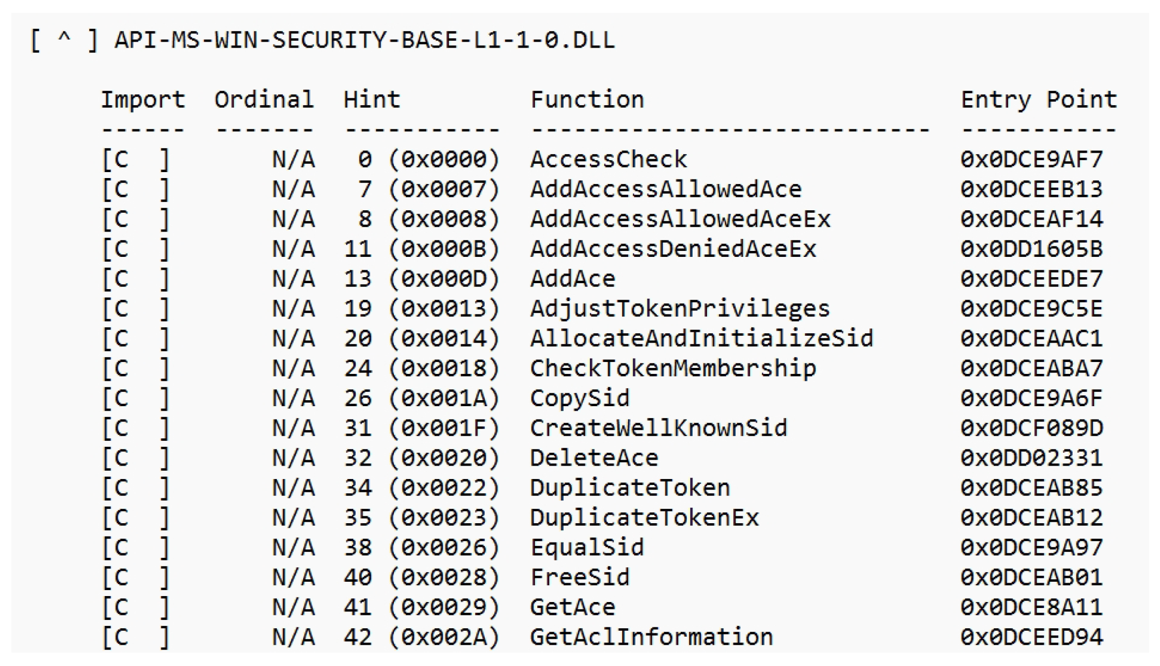
• Static analysis—analysis of a program without executing it. Basic static analysis looks for static information, such as strings, network addresses, called functions, and executable file header information. Advanced static analysis applies reverse engineering techniques using various special tools [7].
• Dynamic analysis—analysis of a program during execution. It is performed in a secure virtual environment, in which the activities of the executed program are observed; these are then used to deduce the purpose of the program [8]. In a secure environment, registry changes, network activity, function calls, disk file modifications, and so on are observed.

Both types of analysis have their advantages and disadvantages. Static analysis is more secure, as malicious code is not directly executed, and it can be used to detect any malicious intent. However, the disadvantage of static analysis lies in its being ineffective against advanced obfuscation techniques aiming to prevent source code analysis [7]. Dynamic analysis allows one to reveal the functionality of a program without the need (eventually) for tedious code analysis. However, to its disadvantage, a secure environment is necessary for its execution [8], as running a malicious sample on a real system could be a risk; moreover, more advanced malware can often detect virtual environments or wait for either a time or a specific event and thus refrain from malicious activity.

2.2. Malware Detection

Currently, these are the most widespread malware detection methods:

• Signature-based detection—the most commonly used malware detection method [9]. Signatures are unique sequences of bytes obtained by malware analysis. These signatures are used to identify a particular piece of malware [8]. Security programs contain a database of signatures of known malware. Whenever a new file is checked, this file is analysed and compared with the database [9]. If the analysed file contains a signature listed in the database, it is highly probable that the file is malicious.
• Behaviour-based detection—during the detection, the behaviour of the program and its activities are examined. Attempts to perform abnormal or unauthorised action could indicate the program is malicious or at least suspicious. Examples of abnormal actions include modifying other files, adding new users to the system, and stopping system security software, to name a few [9].
• Heuristic detection—this means looking for certain features indicating malicious behaviour by using rules and algorithms, either by looking for commands and instructions typical of malware or by monitoring its behaviour and activities during execution, or even—frequently—by a combination of the two [10]. Each activity is then rated in terms of risk, and—if a set threshold is surpassed—preventive action is taken [11].

The most significant disadvantage of signature-recognition-based detection is that it can only detect known malware registered in the signature database [8]. This disadvantage can be observed especially in the case of polymorphic and metamorphic malware. A partial solution to this issue is to use behaviour-based detection and heuristic detection, as these methods are capable of detecting new malware with yet unknown signatures. However, their disadvantage is a higher false positive rate, that is, they tend to mislabel benign programs as malicious ones [8].

2.3. Detection Using Machine Learning

Recent years have seen a boom in the use of machine learning in many fields. Malware detection is no exception to this rule. Here, it tries to address the drawbacks of established detection methods, especially as new malware appears every day. As a result, there is an increased interest of the scientific community in this area, leading to ever growing amounts of reference works. These differ mainly in the algorithms and the types of analysis (static or dynamic) used. Several review studies have already been carried out on this issue. Gibert et al. [12] presented a survey of machine learning techniques for malware detection and, in particular, deep learning techniques. The authors reviewed a total of 67 research papers tackling the problem of malware detection and classification on the Windows platform. The reviewed papers were compared and analysed according to the input features, the classification algorithm, and the characteristics of the dataset. Another systematic review of machine-learning-based Android malware detection techniques was presented by Senanayake et al. [13]. The authors of this article critically evaluated 106 articles, highlighting their strengths and weaknesses as well as potential improvements.

In the following, we describe some existing practically focused works in this domain, specifically considering supervised machine learning.

2.4. Reference Works

Malware detection using machine learning techniques was first addressed by Schultz et al. in their work [14], using static analysis techniques, focusing on features including extracted strings, header information from executable files (the called and imported functions), and a contiguous sequence of n bytes (n-grams). The authors of the aforementioned paper used three machine learning algorithms (RIPPER, naïve Bayes (NB), and multi-NB), complemented with a traditional malware detection method (signature-based detection) for comparison purposes. The overall detection accuracy in their experiments ranged from 83.62% to 97.11% when using machine learning algorithms, which was a significant increase compared to the traditional, signature-based detection, which had an overall accuracy of 49.28%.

The use of static analysis techniques was also discussed by Bai et al. [15]. In their work, they used 197 features extracted from the headers of executable files, namely the number of API calls and the number of dynamically linked libraries used. To select the most appropriate features that could best distinguish between malicious and benign samples, the authors used filtering and wrapper methods. The algorithms used and compared in this work were decision-tree-based algorithms, namely the J48 and random forest (RF) algorithms. By performing several experiments, the authors achieved an overall detection accuracy ranging from 94.6% to 99.1%.

The header information of the executables was also used by Kumar et al. [16], who used an integrated feature set with a total of 68 features. The authors used and compared a total of six algorithms in their work, namely the NB, RF, decision tree (DT), logistic regression (LR), linear discriminant analysis (LDA), and k–nearest neighbors (KNN) algorithms. The overall detection accuracies achieved ranged from 56.04% to 98.78%. The least successful algorithm in the comparison was the NB algorithm, while the most successful algorithm with the best detection accuracy was the RF algorithm.

The features of decompiled machine code—opcode sequences of various lengths—were used by Bragen [17], who also used and compared six algorithms, namely the NB, RF, KNN, multilayer perceptron (MLP), support vector machine (SVM), and J48 algorithms. Again, the most successful algorithm with the best detection accuracy was the RF algorithm, as it achieved a detection accuracy of 95.58% for three-byte sequences (3-grams).

By extracting five-byte sequences (5-grams) and API call information from the headers of the executable files, Chowdhury et al. [18] used and compared the success rates of multiple algorithms, notably the NB, J48, RF, SVM, and MLP. They performed several experiments according to the type of features used. The best detection accuracy (97.7%) was obtained using artificial neural network (ANN) with a feed-forward perceptron and combining both types of features. According to this work, the least successful algorithm was the NB algorithm, with a detection accuracy of 87.5%.

The authors of the aforementioned works extracted the features by using only static analysis techniques. The issue with this malware detection approach was described by Moser et al. [19], citing the use of obfuscation techniques to hide malicious code as the main reason. Thus, they recommend also using dynamic analysis, which is less vulnerable to this problem.

In addition to the features obtained by extracting strings from executables using static analysis techniques, Shijo and Salim [20] also performed dynamic analysis in an isolated virtual environment to obtain information including registry changes and API function call counts. In their work, they compared the RF and SVM algorithms and their success rates in different types of analysis, through several experiments. They obtained the best result (98.7%) by applying the SVM algorithm to features obtained by combining static and dynamic analysis. When applying the algorithm to features obtained by dynamic analysis only, the detection accuracy was slightly worse, specifically 97.1%. Considering static analysis, the detection accuracy was 95.88%. Thus, the achieved results showed that the combination of static and dynamic analysis increased the detection accuracy compared to the use of static and dynamic analysis alone.

The use of dynamic analysis techniques to extract features was also discussed by Firdausi et al. [21], who used the open-source Anubis tool for dynamic analysis. In their work, these authors used and compared a total of five machine learning algorithms—notably NB, SVM, MLP, KNN, and J48—in several experiments. They found the J48 algorithm to be the best (having a 96.8% detection accuracy) and the NB algorithm to be the worst (having a 62.8% detection accuracy).

Mosli et al. [22] used the Cuckoo Sandbox, an automated dynamic malware analysis system, to extract features from memory dumps, which are produced during the execution of the samples. They compared the accuracies of three algorithms: KNN, SVM, and RF. They obtained the best detection accuracy using the RF algorithm, namely 91.4%. The worst results (91% detection accuracy) were obtained using the KNN algorithm.

Kumar and Geetha [23] proposed a malware classification scheme that constructs a model using low-end computing resources and a very large balanced dataset—the EMBER dataset, which consists of 1.1 million entries—for malware. The authors compared the performance of nine algorithms: Gaussian NB, KNN, linear support vector classification (SVC), DT, AdaBoost, RF, extra trees, gradient boost (GDB), and XGBoost. In their experiments, XGBoost outperformed the other algorithms. Therefore, the authors built the final classifier based on XGBoost. Their hyperparameter-tuned model has an accuracy of 98.5% and AUC of 0.9989. This research is unique and significant because it uses an entire dataset with XGBoost using gradient boost decision tree (GBDT) algorithm to get matching or higher accuracy with low computing resources.

The NB, DT, RF, GDB, and XGBoost algorithms were used for developing the classification model for malware detection in the research of Dhamija and Dhamija [24]. They considered five approaches to find out the discerning features for classification. Four approaches were based on the presence of features in malware and/or benign files. The authors, in their fifth approach, use feature selection methods, namely the chi-square, mutual information, and extra trees classifiers. The features obtained from these three classifiers were combined to form a feature set in this approach. The best detection accuracy was 99.5% for both RF and XGBoost.

Shhadat et al. [25] applied seven learning algorithms on a benchmark dataset in their experiments, namely KNN, SVM, Bernoulli NB, RF, DT, logistic regression (LR), and hard voting (HV) on particular classification algorithms: LR, SVM, Bernoulli NB, and DT. This paper shows that the highest accuracy was achieved by DT, with a score 98.2% for binary classification and 95.8% by RF for multi-class classification. The lowest accuracy was achieved by Bernoulli NB, with an accuracy of 91% and 81.8% for binary classification and multi-class classification, respectively.

An overview of the existing works is available in

Table 1. Overview of existing works.

Work	Analysis Type	Dataset Size (Malicious/Clean)	Algorithms Compared	Best Accuracy (%)	Best Sensitivity (%)
Schultz et al. [14]	static	3265/1001	RIPPER, NB, Multi-NB	97.11	97.43
Bai et al. [15]	static	10,521/8592	J48, RF	95.1–99.1	91.3–99.1
Kumar et al. [16]	static	2722/2488	RF, DT, LR, NB, LDA, KNN	98.78	99.0
Bragen [17]	static	992/771	RF, NB, KNN, SVM, J48, ANN	95.58	96.77
Chowdhury et al. [18]	static	41,265/10,920	NB, J48, RF, SVM, ANN	97.7	91
Shijo, Salim [20]	static	997/490	SVM, RF	95.88	95.9
Shijo, Salim [20]	dynamic	997/490	SVM, RF	97.16	97.2
Shijo, Salim [20]	combined	997/490	SVM, RF	98.71	98.7
Firdausi et al. [21]	dynamic	220/250	NB, SVM, MLP, KNN, J48	96.8	95.9
Mosli et al. [22]	dynamic	3130/1157	KNN, SVM, RF	91.4	91.1
Kumar, Geetha [23]	Ember dataset	300 K/300 K	Gaussian NB, KNN, Linear SVC, DT, AdaBoost, RF, Extra Trees, GB, XGBoost	98.5	0.89–0.99
Dhamija, Dhamija [24]	open data source	4060/2709	NB, DT, RF, GB, XGBoost	99.95	-
Shhadat et al. [25]	open data source	984/172	KNN, SVM, Bernoulli NB, RF, DT, LR, HV	98.2	92

.

3. Design Methods

It is clear that using machine learning to detect malware has the advantage of good detection accuracy. Existing research also shows that using decision trees to detect malware seems to be a suitable approach, due to its accuracy in detecting malicious samples. Detection accuracy can also be increased by combining multiple models, as is evident in the case of the RF algorithm.

For the above reasons, we chose decision-tree-based algorithms for our program. Thus, the next section contains a description of the steps of supervised machine learning, namely:

• Data acquisition and processing into a suitable form to train the machine learning models;
• Training the models on the training data and finding the best hyperparameters for the particular model;
• Evaluating the models using test data and comparing them.

These steps result in trained models capable of making classifications even on the previously unknown samples utilised in our malware detection program.

3.1. Experimental Hardware Environment

This section describes the hardware used for all tasks performed. The used workstation had the following specifications:

• Processor: Intel(R) Core(TM) i5-9500 CPU @ 3.00GHz;
• Memory: 16 GB DDR4;
• Hard drive: Samsung SSD 860 PRO 512GB, Samsung SSD 970 EVO Plus 500GB;
• GPU: NVIDIA GeForce RTX 3060 12 GB.

3.2. Obtaining the Training Samples

The set of samples for training and testing the classification models includes a total of 3838 executable files—3000 malicious and 838 benign. The malicious samples come from the VirusShare repository [26] of real malicious samples intended for the research community and the like. The particular downloaded package was VirusShare_00164.zip, containing a total of 65,536 malicious samples; of these, we selected 3000 executable files, in both exe and msi format. The benign samples were taken from the PortableFreeware [27] and PortableApps [28] repositories, from which a total of 838 benign samples in both exe and msi formats were downloaded.

3.3. Static Analysis of the Samples

To perform static analysis of the particular programs (i.e., without executing them), we used the Dependency Walker tool. We stored and subsequently processed its outputs into a dataset.

3.3.1. Dependency Walker

Dependency Walker [29] is a freely available program created by Microsoft. It is a tool used to analyse executable files, providing detailed information about the scanned file, including information about the imported modules and functions.

3.3.2. Processing the Output and Creating the Dataset

We used the Dependency Walker tool to perform a static analysis of all samples and to store the output of each analysis in text files containing the imported and exported functions of the respective modules, as shown in Figure 1. The features we focused on were 112 selected functions, most commonly imported by malicious programs. Their names were thus used as the dataset columns. Then, the number of imports of the particular functions was written into the corresponding column (bearing the name of that function) of the dataset. We appended a column entitled malware to the dataset. The values in the corresponding rows were either ‘1’ (in the case of malicious samples) or ‘0’ (in the case of benign samples).

In some cases, we could not perform static analysis using Dependency Walker, due to the incorrect format of the test file and the missing modules, so these outputs were not analysed. After the processing, the training and testing dataset, with 3584 rows in total, was saved in csv format. The composition of the dataset is shown in

Table 2. Composition of the dataset after static analysis.

Class	Count
Malicious	2747
Benign	837
Total	3584

.

3.4. Dynamic Analysis of the Samples

Dynamic analysis was performed by running and observing the behaviour of individual samples in a secure virtual environment, provided by the Cuckoo Sandbox tool. The result of the analysis of the corresponding sample was then stored in a report file, from which the features were extracted into a dataset. As features, we used the call counts of the 298 Windows API functions called during the execution of the respective samples. We focused on all functions that were found during the analysis of the malicious samples.

3.4.1. Cuckoo Sandbox

Cuckoo Sandbox [30] is an open-source tool to analyse executable and other files or web pages in an isolated environment. After initiating the analysis using a web interface or a REST API, the system collects runtime information including the files created, deleted, or downloaded during execution, memory handling, system function calls, network activity, and so on. The collected information is then also accessible via a graphical web interface or a REST API.

The tool includes central management software [30] controlling the triggering and the collection of the sample analysis results. The latter is performed in an isolated environment—this may be a virtual or a physical device or multiple devices.

3.4.2. Dynamic Analysis Test Environment

To perform dynamic analysis, the Cuckoo Sandbox tool has to be configured correctly, and virtual devices to run the dynamic analysis of the sample have to be created. The test environment is shown in Figure 2. Its key parts are as follows:

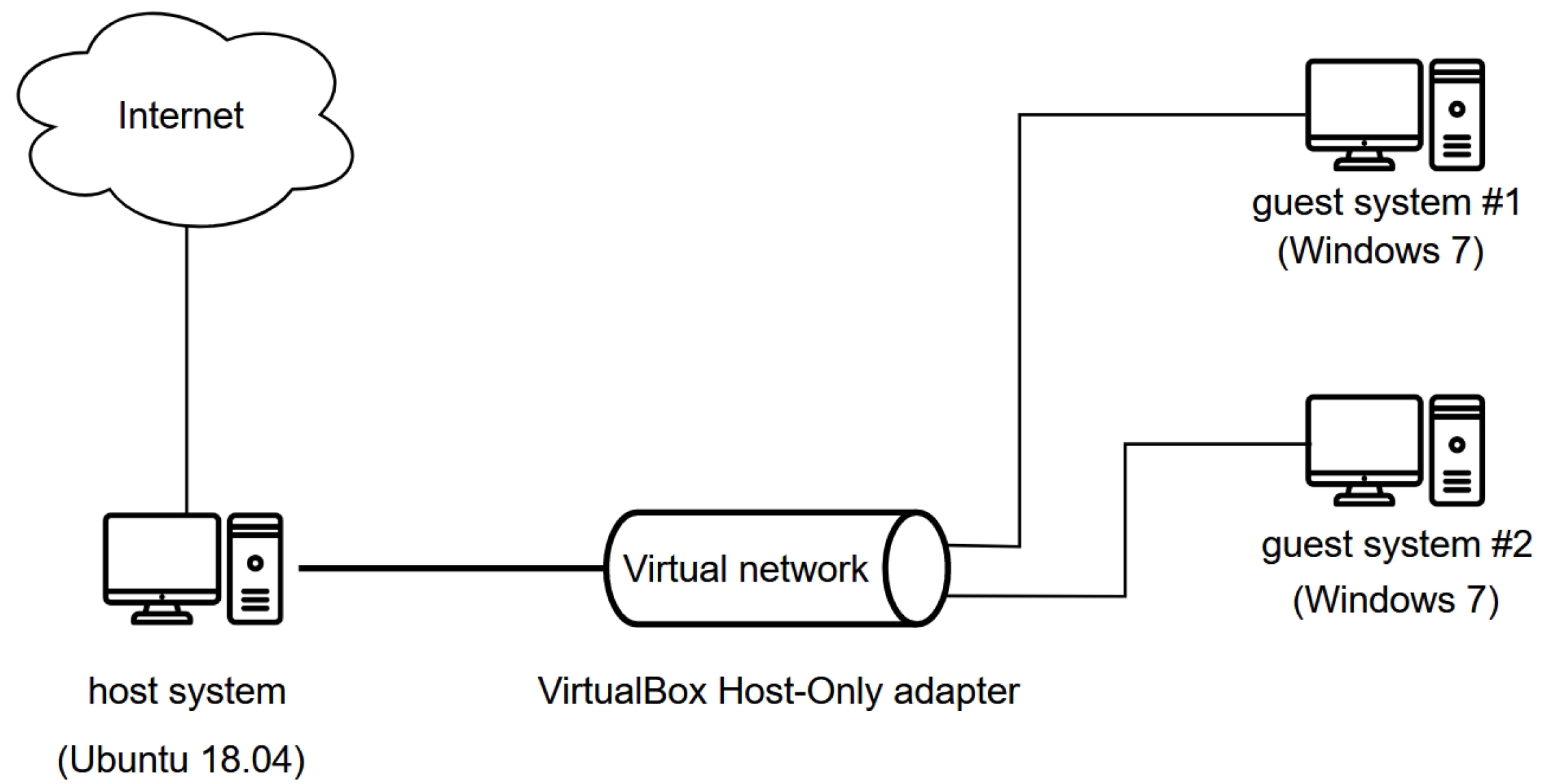
• A host system running Ubuntu 18.04 LTS. This operating system contains Python version 2.7, an installation prerequisite of the Cuckoo Sandbox tool. This system contains the aforementioned central management software that manages the dynamic analysis, accessible through port 8090 of the localhost server, using a REST API.
• A guest system running Windows 7—in our case, two virtual machines created using the VMCloak tool. On these, we performed the dynamic analysis of the samples. We stored the clean, post-installation state of these systems as an environment snapshot. After the analysis, this environment snapshot was automatically restored, as the execution of the malicious samples may have disrupted the environment. Since the operating system inherently contains security mechanisms that could prevent malicious activity from being performed during dynamic analysis, the Windows Defender, Windows Firewall, and Windows Update security mechanisms were disabled on both guest systems. The virtual machines could access the Internet using the VirtualBox host-only adapter.

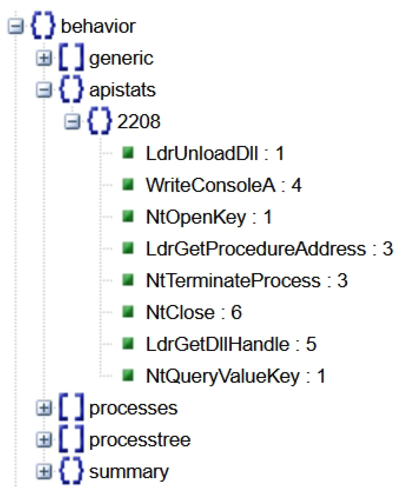
3.4.3. Obtaining and Processing the Output, Creating the Dataset

To work with the Cuckoo Sandbox tool, we used the requests Python library: we sent HTTP requests to the system endpoints containing the central management software (the host system), which collects the analysis results. We used four methods of the CuckooAPI class, implemented by us, to work with the Cuckoo Sandbox tool, namely:

• A method to submit a file for analysis (submit_file), returning the assigned ID;
• A method to submit a URL for analysis (submit_url), also returning the assigned ID;
• A method to find out the analysis status (get_status), returning the status of the analysis with the given ID;
• A method to retrieve the final analysis report (save_report) in JSON format.

After retrieving the result of the dynamic analysis in JSON format, it is processed by a Python script to find the number of calls to each of the 298 selected Windows API functions. These thus constitute the features of the dataset; their names are stored in the dataset header. The names of the functions and their runtime call counts are stored in the output JSON file, in the behavior object and its nested objects, as shown in Figure 3. If a particular function is found, the value in the corresponding column of the dataset is updated by the number of calls to that function, otherwise a ‘0’ value is written to the corresponding field. After the runtime call counts of all functions have been determined, the value of the malware column is stored—either ‘1’ (in the case of malicious samples) or ‘0’ (in the case of benign samples).

As in the case of static analysis, in some cases, dynamic analysis failed, as the format of the sample processed by Cuckoo Sandbox was incorrect, so these outputs were not processed. After the processing, the training and testing dataset, with 3765 rows in total, was saved in csv format. The composition of the dataset is shown in

Table 3. Composition of the dataset after dynamic analysis.

Class	Count
Malicious	2937
Benign	828
Total	3765

.

3.5. Training and Testing Classification Models

In this paper, we analyse the use of two supervised machine learning algorithms. Both are based on decision trees, the use of which seems very appropriate based on the results in existing research, in which decision-tree-based algorithms performed best. These algorithms are the following:

• Extremely randomized trees (ET for short), implemented using the ExtraTreesClassifier class of the Scikit-learn package;
• Extreme gradient boosting (XGBoost for short), implemented using the XGBClassifier class from the xgboost package.

Both datasets were split using the train_test_split method from the Scikit-learn package, with 75% of the data used for training and 25% for testing. We tested several values of the hyperparameters listed in

Table 4. Tested hyperparameters of the ExtraTreesClassifier classifier.

Hyperparameter	Value
criterion	gini; entropy
n_estimators	10; 50; 100; 150; 200; 300
min_samples_split	2; 3; 4; 5
min_samples_leaf	1; 2; 3; 5
max_features	auto; sqrt; log2; None
class_weight	balanced; balanced_subsample; None
max_depth	3; 5; 8; None

and

Table 5. Tested hyperparameters of the XGBClassifier classifier.

Hyperparameter	Value
n_estimators	10; 50; 100; 150; 200; 250; 300
max_depth	3; 5; 7; 9; 11
learning_rate	0.001; 0.01; 0.1; 0.2; 0.3
colsample_bytree	0.3; 0.7; 1
subsample	0.5; 1
scale_pos_weight	0.3
gamma	0; 1; 2; 3

. For each combination of hyperparameters, we repeated training and testing 20 times. The classification model training based on XGBoost for 20 iterations in our hardware environment took 16 h and 23 min. Training the ET model took 15 h and 45 min. It is worth mentioning that the training time also depends on the CPU utilization. The results obtained were written into a single csv file.

3.6. Evaluation of the Models

We calculated the mean values of the respective results of the 20 iterations, obtained for each combination of hyperparameters, and calculated the standard deviation values. We ranked them from best to worst with respect to the classification accuracy metric. Complementary to the metrics listed above were the specificity and sensitivity metrics.

3.6.1. Evaluation Metrics

The metrics we used are derived and can be calculated from the confusion matrix shown in Figure 4, according to which the classification result can be evaluated as necessary. It contains the following values [31]:

• True negative (TN)—the number of correctly identified benign samples;
• True positive (TP)—the number of correctly identified malicious samples;
• False positive (FP)—the number of incorrectly identified malicious samples;
• False negative (FN)—the number of incorrectly identified benign samples.

Classification Accuracy

Classification accuracy expresses the number of samples—compared to the total number of samples—that were classified correctly. It is expressed as follows:

$$\mathrm{Accuracy}=\frac{TP+TN}{TP+FP+TN+FN}$$

(1)

Precision

Precision expresses how many samples of all positive samples were correctly predicted as positive. It is the first part of F1 score. It is expressed as follows:

$$\mathrm{Precision}=\frac{TP}{TP+FP}$$

(2)

Sensitivity (aka Recall)

Sensitivity (recall) expresses the ability of the model to correctly classify positive (in our case: malicious) samples, that is, it expresses how many samples of all positive samples were correctly classified as positive. A model with high sensitivity succeeds well in finding all the positive cases in the data. It is the second part of F1 score. It is expressed as follows:

$$\mathrm{Sensitivity}=\mathrm{Recall}=\frac{TP}{TP+FN}$$

(3)

Specificity

Specificity expresses the ability of the model to correctly classify negative (in our case: benign) samples, that is, it expresses how many samples of all negative samples were correctly classified as negative. It is expressed as follows:

$$\mathrm{Specificity}=\frac{TN}{TN+FP}$$

(4)

F1 Score

Precision and recall are the two most common metrics that take into account class imbalance. F1 score expresses the harmonic mean between recall and precision values. The goal of the F1 score is to combine the precision and recall metrics into a single metric. It is expressed as follows:

$$\mathrm{F}1\mathrm{score}=\frac{2\ast \mathrm{Precision}\ast \mathrm{Recall}}{\mathrm{Precision}+\mathrm{Recall}}$$

(5)

Area under the Curve

The area under the curve (AUC) is an aggregated measure of the performance of a binary classifier on all possible threshold values of the receiver operating characteristics curve (ROC). It is calculated as the area under this ROC. The AUC ranges from 0 to 1. The bigger the AUC score, the better our classifier is.

3.6.2. Extremely Randomized Trees

Table 6. Best results for the extremely randomized trees algorithm (static analysis).

Parameters	Classification Accuracy (%)	Sensitivity (%)	Specificity (%)	ROC AUC	F1
ET_S_1	$91.786\pm 0.697$	$97.176\pm 0.890$	$74.067\pm 3.107$	$0.856\pm 0.014$	$0.948\pm 0.017$
ET_S_2	$91.775\pm 0.623$	$97.322\pm 0.817$	$73.541\pm 3.326$	$0.854\pm 0.014$	$0.948\pm 0.016$
ET_S_3	$91.774\pm 0.625$	$97.489\pm 0.845$	$72.990\pm 3.239$	$0.852\pm 0.014$	$0.948\pm 0.017$
ET_S_4	$91.769\pm 0.650$	$97.445\pm 0.853$	$73.110\pm 3.295$	$0.853\pm 0.014$	$0.948\pm 0.016$
ET_S_5	$91.769\pm 0.676$	$97.198\pm 0.838$	$73.923\pm 3.403$	$0.856\pm 0.015$	$0.948\pm 0.017$

shows the top five results obtained by applying the ET algorithm to the static analysis data. In the best case, the mean classification accuracy was 91.786%, with a mean sensitivity of 97.176% and a mean specificity of 74.067%. Recall–the part of the F1 score that takes into account not only the number of prediction errors that the model makes, but also looks at the type of errors that are made—achieved a value of 0.948. The AUC was 0.856. Slightly better results were obtained by applying this algorithm to the dynamic analysis data shown in

Table 7. Best results for the extremely randomized trees algorithm (dynamic analysis).

Parameters	Classification Accuracy (%)	Sensitivity (%)	Specificity (%)	ROC AUC	F1
ET_D_1	$96.387\pm 0.685$	$98.165\pm 0.497$	$90.281\pm 2.302$	$0.942\pm 0.012$	$0.977\pm 0.010$
ET_D_2	$96.375\pm 0.530$	$98.039\pm 0.525$	$90.663\pm 1.753$	$0.944\pm 0.009$	$0.977\pm 0.010$
ET_D_3	$96.375\pm 0.540$	$98.202\pm 0.568$	$90.102\pm 1.530$	$0.942\pm 0.008$	$0.977\pm 0.011$
ET_D_4	$96.375\pm 0.705$	$98.016\pm 0.495$	$90.740\pm 2.229$	$0.944\pm 0.012$	$0.977\pm 0.010$
ET_D_5	$96.375\pm 0.605$	$97.875\pm 0.510$	$91.224\pm 1.832$	$0.945\pm 0.010$	$0.977\pm 0.010$

. With these data, in the best case, the mean classification accuracy was 96.387%, with a mean sensitivity of 98.168% and a mean specificity of 90.281%. As far as static analysis data are concerned, the specificity metric showed lower values, which is associated with a larger number of false positives and thus lower classification accuracy. The F1 score was 0.977 and the AUC 0.942. Both metrics achieved a slightly better score compared to the ET algorithm realized on the data coming from the static analysis. This was caused by the different proportions of malware and benign files in the data sets.

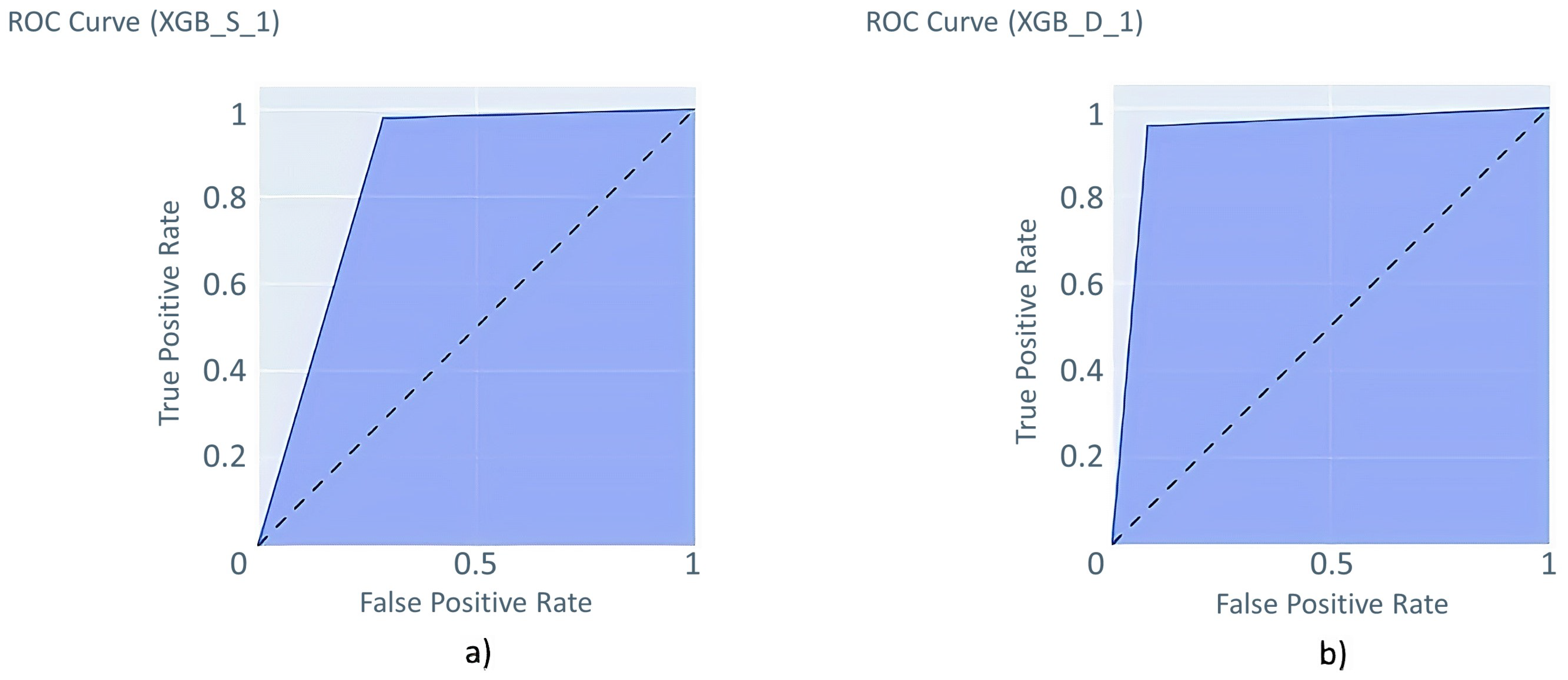
3.6.3. Extreme Gradient Boosting

The XGBoost algorithm performed slightly better on both static and dynamic analysis data. Considering static analysis, as shown in

Table 8. Best results for the XGBoost algorithm (static analysis).

Parameters	Classification Accuracy (%)	Sensitivity (%)	Specificity (%)	ROC AUC	F1
XGB_S_1	$91.920\pm 0.658$	$98.253\pm 0.472$	$71.100\pm 3.051$	$0.847\pm 0.014$	$0.949\pm 0.009$
XGB_S_2	$91.914\pm 0.617$	$98.508\pm 0.380$	$70.239\pm 2.762$	$0.844\pm 0.013$	$0.949\pm 0.008$
XGB_S_3	$91.897\pm 0.609$	$98.231\pm 0.426$	$71.077\pm 2.980$	$0.847\pm 0.014$	$0.949\pm 0.008$
XGB_S_4	$91.858\pm 0.635$	$98.464\pm 0.452$	$70.143\pm 3.048$	$0.843\pm 0.014$	$0.949\pm 0.009$
XGB_S_5	$91.853\pm 0.717$	$97.584\pm 0.492$	$73.014\pm 3.338$	$0.853\pm 0.016$	$0.948\pm 0.010$

, in the best case, the mean classification accuracy was 91.920%, the mean sensitivity was 98.253%, and the mean specificity was 71.100%. The best XGB model trained on features from the static analysis achieved an F1 score of 0.949 and 0.847 AUC. Considering dynamic analysis, as shown in

Table 9. Best results for the XGBoost algorithm (dynamic analysis).

Parameters	Classification Accuracy (%)	Sensitivity (%)	Specificity (%)	ROC AUC	F1
XGB_D_1	$96.467\pm 0.560$	$98.514\pm 0.602$	$89.439\pm 2.484$	$0.940\pm 0.011$	$0.977\pm 0.012$
XGB_D_2	$96.438\pm 0.522$	$98.670\pm 0.780$	$88.776\pm 2.499$	$0.937\pm 0.011$	$0.977\pm 0.015$
XGB_D_3	$96.387\pm 0.517$	$98.789\pm 0.722$	$88.138\pm 2.466$	$0.935\pm 0.011$	$0.977\pm 0.014$
XGB_D_4	$96.381\pm 0.521$	$98.782\pm 0.563$	$88.138\pm 2.482$	$0.935\pm 0.011$	$0.977\pm 0.011$
XGB_D_5	$96.341\pm 0.529$	$98.841\pm 0.559$	$87.755\pm 2.382$	$0.933\pm 0.011$	$0.977\pm 0.011$

, in the best case, the mean classification accuracy was 96.467%, the mean sensitivity was 98.514%, the mean specificity was 89.439%, the F1 score was 0.977, and the AUC was 0.940. The values obtained for the F1 metric and for the AUC are very similar to the values obtained by ET in both (static, dynamic) cases.

3.7. Choosing the Best Model

Using several metrics, we compared the best results with the results of our previous works, in which we compared multiple algorithms—RF, DT, SVM, and NB—on the same dataset.

Table 10. Comparison of the best results for each algorithm (static analysis).

Algorithm	Classification Accuracy (%)	Sensitivity (%)	Specificity (%)	ROC AUC
XGB	$91.92\pm 0.66$	$98.25\pm 0.47$	$71.10\pm 3.05$	$0.85\pm 0.01$
ET	$91.79\pm 0.70$	$97.18\pm 0.89$	$74.07\pm 3.11$	$0.86\pm 0.01$
RF	$91.32\pm 0.92$	$96.94\pm 0.60$	$72.82\pm 2.93$	$0.85\pm 0.02$
DT	$89.74\pm 0.98$	$95.76\pm 1.08$	$69.97\pm 2.56$	$0.83\pm 0.01$
SVM (poly)	$88.48\pm 0.78$	$95.46\pm 0.66$	$65.55\pm 2.54$	$0.81\pm 0.01$
SVM (rbf)	$88.11\pm 0.61$	$96.69\pm 0.65$	$59.94\pm 2.50$	$0.78\pm 0.01$
SVM (linear)	$87.94\pm 1.02$	$95.75\pm 0.86$	$62.25\pm 4.16$	$0.79\pm 0.02$
NB	$42.27\pm 1.28$	$26.61\pm 1.66$	$93.72\pm 1.11$	$0.60\pm 0.01$

shows a comparison of the best results for each of the algorithms implemented herein and in our previous work [32], using the dataset obtained by static analysis of the samples using Dependency Walker. The results are ranked according to the classification accuracy metric from best to worst.

Similarly,

Table 11. Comparison of the best results for each algorithm (dynamic analysis).

Algorithm	Classification Accuracy (%)	Sensitivity (%)	Specificity (%)	ROC AUC
XGB	$96.47\pm 0.56$	$98.51\pm 0.60$	$89.44\pm 2.48$	$0.94\pm 0.01$
ET	$96.39\pm 0.68$	$98.16\pm 0.50$	$90.28\pm 2.30$	$0.94\pm 0.01$
RFC	$95.95\pm 0.58$	$98.08\pm 0.49$	$88.66\pm 2.34$	$0.94\pm 0.01$
DT	$94.53\pm 0.74$	$96.37\pm 0.73$	$88.20\pm 2.53$	$0.92\pm 0.01$
SVM (linear)	$92.38\pm 0.83$	$97.82\pm 0.62$	$73.69\pm 2.88$	$0.86\pm 0.01$
SVM (poly)	$92.17\pm 0.79$	$97.60\pm 0.69$	$73.54\pm 3.15$	$0.86\pm 0.02$
SVM (rbf)	$91.93\pm 0.84$	$98.68\pm 0.50$	$68.76\pm 3.17$	$0.84\pm 0.02$
NB	$59.53\pm 1.76$	$48.58\pm 2.42$	$97.14\pm 1.31$	$0.73\pm 0.01$

shows a comparison of the best results for each of the algorithms implemented herein and in our previous work [33], using the dataset obtained by dynamic analysis of the samples using Cuckoo Sandbox. Again, the results are ranked according to the classification accuracy metric from best to worst.

Since in the proposed program, our main goal was to correctly detect as many malicious samples as possible, the main compared metric was the sensitivity metric. The XGBoost algorithm performs better than the other algorithms, in both cases. Thus, we then exported and stored the models containing a combination of hyperparameters achieving the best results (denoted as XGB_S_1 in Table 8 and XGB_D_1 in Table 9) using the joblib library, for further use. The hyperparameter values for these models are shown in

Table 12. Values of the tested hyperparameters of the best models.

Model	n_estimators	max_depth	learning_rate	colsample_bytree	subsample	scale_pos_weight	gamma
XGB_S_1	300	11	0.01	0.7	1	0.3	1
XGB_D_1	300	11	0.01	0.3	1	0.3	0

. The receiver operating characteristics curve (ROC) for these models are shown on Figure 5

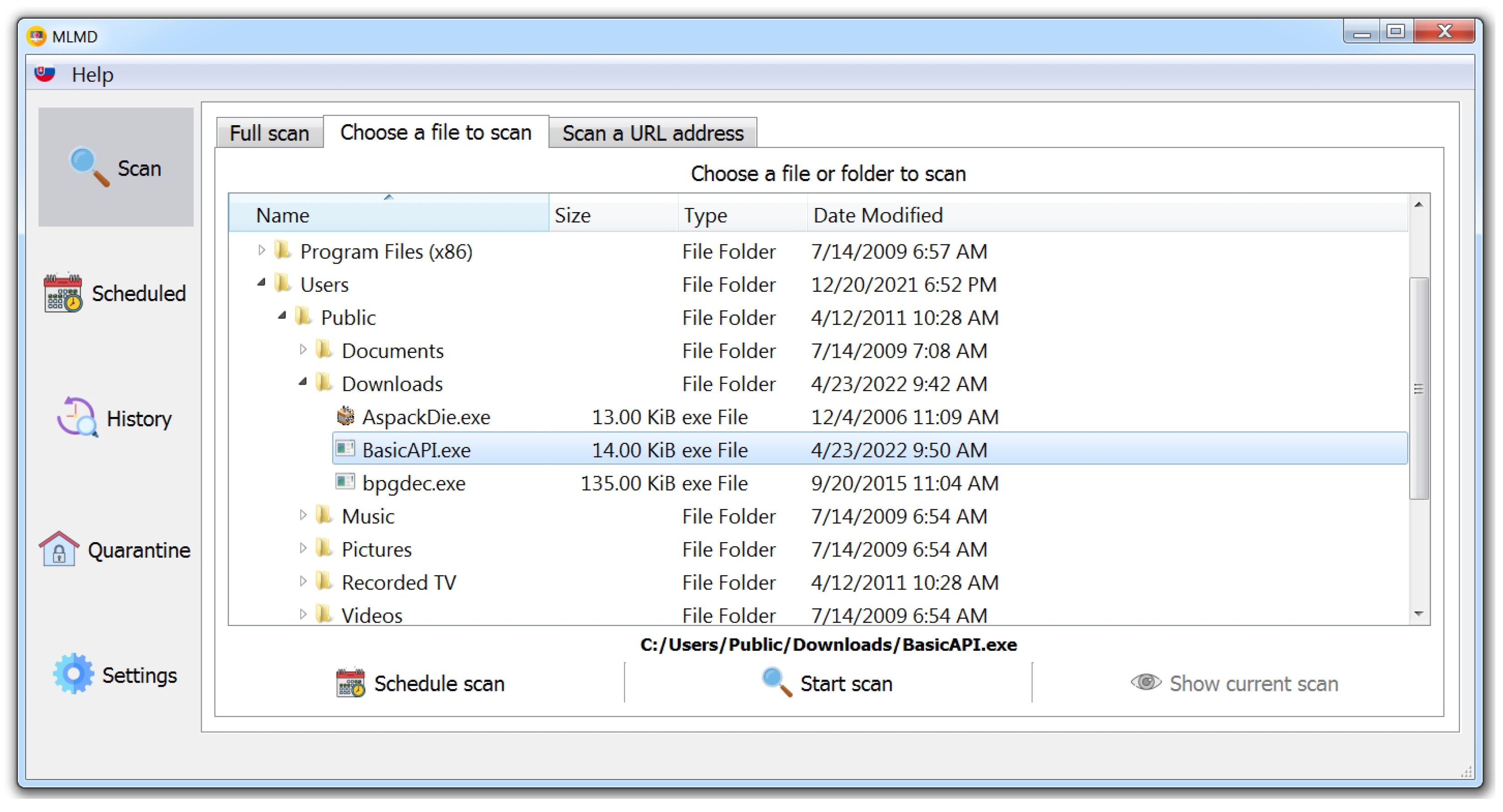
3.8. The Program and Its User Interface

To apply the trained models to classify new samples, we designed a program with a graphical user interface to make scanning of new executables easier. In addition, it also offers other functionalities, such as the following:

• Scanning of multiple files in a folder or the whole system;
• Quarantining malicious executable files;
• Scheduled scanning according to user-specified conditions.

Further features are scanning and classification of web sites using the Cuckoo Sandbox, which also offers such functionality.

We created the graphical user interface using the PyQt5 Python library. The program is composed of several basic windows, complemented by additional modal windows. The basic window of the program consists of the following:

• A screen to select a file or to enter a URL to be scanned or to scan the entire system;
• A screen showing an overview of scheduled one-time or repeated scans of files and folders;
• A screen showing an overview of already completed scans;
• A screen showing quarantined files;
• A screen to view and change program settings.

The main window of the program consists of a screen to select a file or to enter a URL to be scanned or to scan the entire system. This is depicted in Figure 6. It appears upon program start-up.

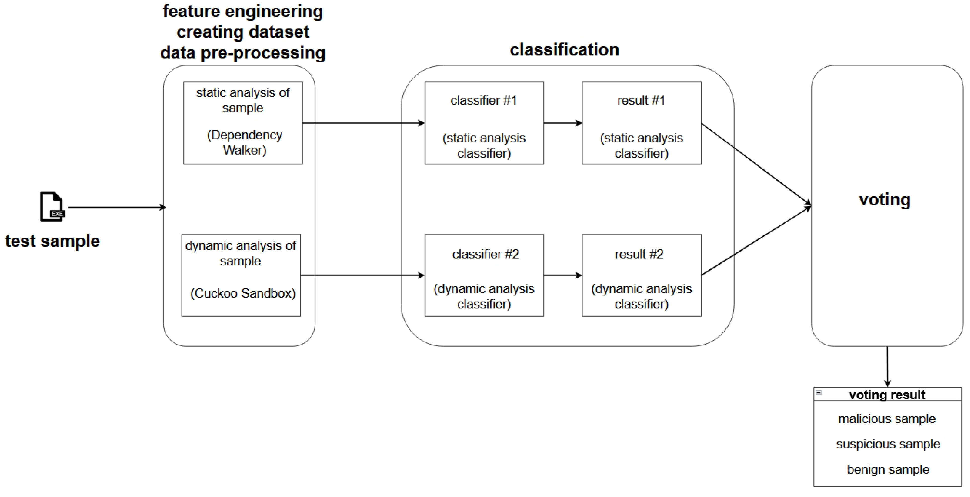
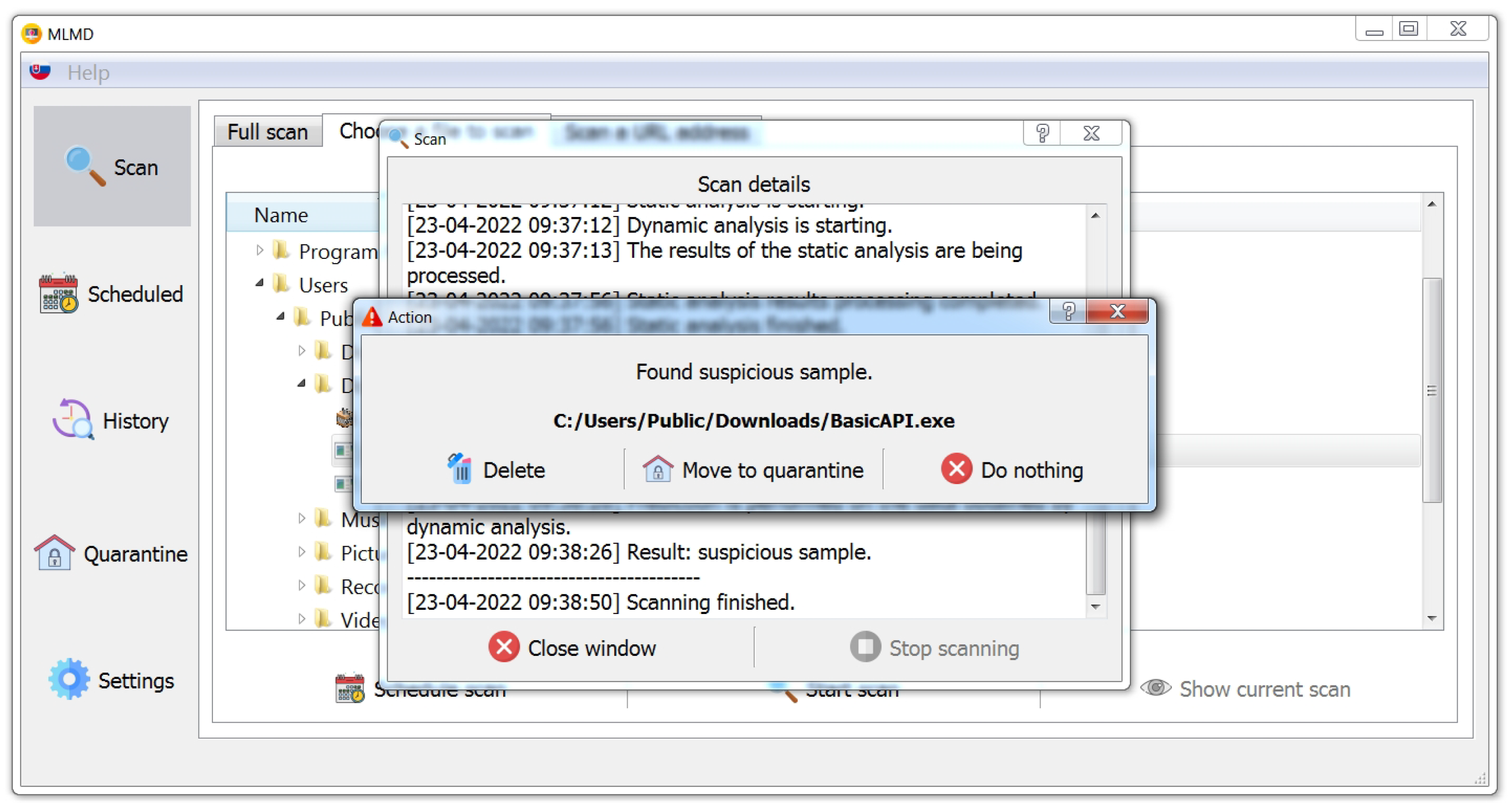
3.8.1. Scanning a File

After initiating the scanning of the test sample, the following steps are performed:

• Static analysis using Dependency Walker and dynamic analysis using Cuckoo Sandbox, resulting in two analysis outputs. From these, the features are extracted and the dataset is created (as in the case of the training data).
• Loading the two machine learning classifiers trained on the training data, separately, for the dataset obtained by static analysis and for the dataset obtained by dynamic analysis.
• Classification itself.
• Combining the obtained results (voting) to decide on the malicious, suspicious, or benign nature of the test sample.

This sequence of steps is shown in Figure 7.

Obtaining the Final Result—Malicious/Benign Nature

The classifier assigns a value of ‘1’ if the sample is malicious and ‘0’ if the sample is benign. As the detection system consists of two classifiers, their results have to be combined to determine the result, as shown in

Table 13. Obtaining the final result of the classification concerning a file.

Result (Static Analysis)	Result (Dynamic Analysis)	Final Result
malicious (1)	malicious (1)	malicious
malicious (1)	benign (0)	suspicious
benign (0)	malicious (1)	suspicious
benign (0)	benign (0)	benign

.

After evaluating the maliciousness of a sample, if a malicious or suspicious sample is found, the user is prompted to select the action to be performed with the scanned file, as shown in Figure 8.

3.8.2. Scanning a Web Address

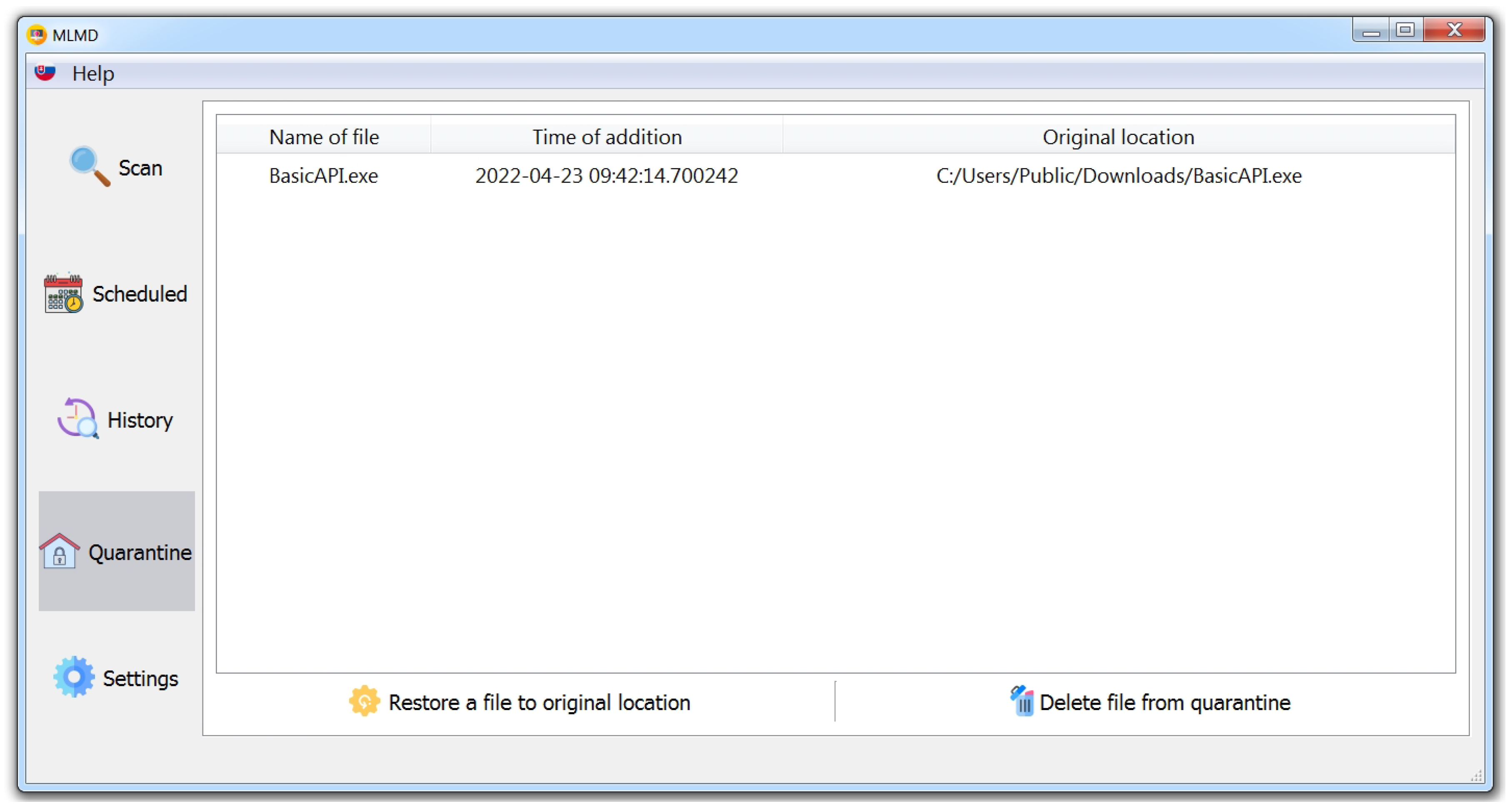
URL scanning is an additional feature of the program, using and mediating the functionality of the Cuckoo Sandbox tool. In addition to the analysis of files of various formats, this tool also allows the input of a URL, which is then visited in a browser and analysed in an isolated virtual system environment. Once the analysis is complete, the result is returned in the form of a JSON file containing the resulting score, ranging from 0 to 10 (in the info object), a description of the threats found, and their severity (the signatures array), as shown in Figure 9. As to the values, 0 indicates the lowest threat level, and 10 the highest level.

Finally, the user sees the resulting score and a verbal rating, as depicted in

Table 14. The final score of URL scanning.

Maliciousness Score (0 = min., 10 = max.)	Final Result
0 ≤ score < 4	secure
4 ≥ score < 7	suspicious
7 ≥ score ≤ 10	very suspicious

.

3.8.3. Quarantine

If a suspicious or potentially malicious file is detected, many antivirus solutions allow quarantining the file in order to prevent its execution and thus its spread to other parts of the system. The quarantined files are not deleted, but moved to a folder hidden from the users and—eventually—modified to prevent them from being executed. The user can then (for example, based on additional information about the file) decide whether to keep the quarantined file, to remove it from the quarantine and from the entire system, or to restore it to its original location in the system.

Our program uses the Quarantine folder, located in the project directory. It is used to preserve files moved by the program or by the user. The files in this folder are encoded using base64 encoding and stored in .b64 format. The steps of quarantining a file are as follows (similarly, recovering a file from the quarantine is performed by decoding it):

• Opening the original file in read binary mode;
• Opening a new file in write binary mode in the Quarantine folder;
• Reading the original file line by line and transforming (encoding) it using the base64io library;
• Writing each transformed line to the new file;
• Deleting the original file.

The program includes a screen providing an overview of the quarantined files. This allows the user to restore them to their original locations and permanently remove them from the quarantine, as depicted in Figure 10.

4. Evaluation

To evaluate the success rate, we compared our results with the following:

• Existing studies, mentioned at the beginning hereof;
• The free VirusTotal tool.

4.1. Comparison with Existing Studies

Table 15. Comparison with existing studies.

Work	Analysis Type	Dataset Size (Malicious/Clean)	Best Algorithm	Accuracy (%)	Sensitivity (%)
Schultz a kol. [14]	static	3265/1001	RF	97.11	97.43
Bai a kol. [15]	static	10,521/8592	J48	95.1–99.1	91.3–99.1
Kumar a kol. [16]	static	2722/2488	RF	98.78	99.0
Bragen [17]	static	992/771	RF	95.58	96.77
Chowdhury a kol. [18]	static	41,265/10,920	ANN	97.7	91
Shijo a Salim [20]	static	997/490	SVM	95.88	95.9
This study	static	2747/837	XGBoost	91.92	98.25
This study	dynamic	2937/828	XGBoost	96.48	98.51
Shijo a Salim [20]	dynamic	997/490	SVM	97.16	97.2
Shijo a Salim [20]	combined	997/490	SVM	98.71	98.7
Firdausi a kol. [21]	dynamic	220/250	J48	96.8	95.9
Mosli a kol. [22]	dynamic	3130/1157	RF	91.4	91.1
Kumar and Geetha [23]	Ember dataset	300 K/300 K	Gaussian NB, KNN, Linear SVC, DT, AdaBoost, RF, Extra Trees, GB, XGBoost	98.5	0.89–0.99
Dhamija and Dhamija [24]	Open data source	4060/2709	NB, DT, RF, GB, XGBoost	99.95	-
Shhadat et al. [25]	Open data source	984/172	KNN, SVM, Bernoulli NB, RF, DT, LR, HV	98.2	92

shows a comparison with existing studies, mentioned earlier. It shows the accuracy and sensitivity values applicable to the best cases, using the algorithms presented. Our accuracy and sensitivity values are expressed as arithmetic mean values. They were obtained by testing during the respective iterations and during the search for the best parameters on a specially crafted dataset (25% of the original dataset).

We have achieved particularly good results in terms of the sensitivity metric, so we can classify malicious samples well, while maintaining a low false negative rate. For the dataset obtained by static sample analysis, we lag behind slightly in terms of classification accuracy—this is mainly related to the number of false positives, which we attribute to the imbalanced data. In the case of the dataset obtained by dynamic sample analysis, the results are slightly better than those obtained by static analysis, which may be due to a better selection of features to distinguish between malicious and benign samples in the case of the data obtained by dynamic analysis.

4.2. Comparison of MLMD and VirusTotal

VirusTotal is one of the most popular online tools to scan suspicious files and websites. It is a kind of information aggregator combining the output of various—currently more than 70—antivirus products. The following comparison is a comparison of the output of our own MLMD program with the output of VirusTotal.

4.2.1. Test Samples

The test suite consisted of 105 samples. Its composition in terms of maliciousness is shown in

Table 16. Test sample composition.

Class	Count
Malicious	70
Benign	35
Total	105

.

The malicious samples consisted of executables downloaded from the VirusShare repository of malicious samples, namely the VirusShare_00164.zip package. The maliciousness was assessed by the VirusShare repository. This was also used to obtain our training data. As the aforementioned package contains a total of 65,536 malicious samples, and we only used the first 3000 samples for training, we selected samples that were not used in training our machine learning models. The benign samples also consisted of executables randomly selected from the free PortableApps site.

We tested each test sample with both our program and the VirusTotal tool. After testing a particular sample by our program, we recorded one of the following results:

• Malicious—both classification models classified the sample as malicious;
• Suspicious—one classification model classified the sample as malicious, the other as benign;
• Benign—both classification models classified the sample as benign.

In case of the VirusTotal tool, the score, recorded for the respective sample, consisted of the following:

• The number of systems that detected the sample as malicious;
• The number of systems that detected the sample as benign.

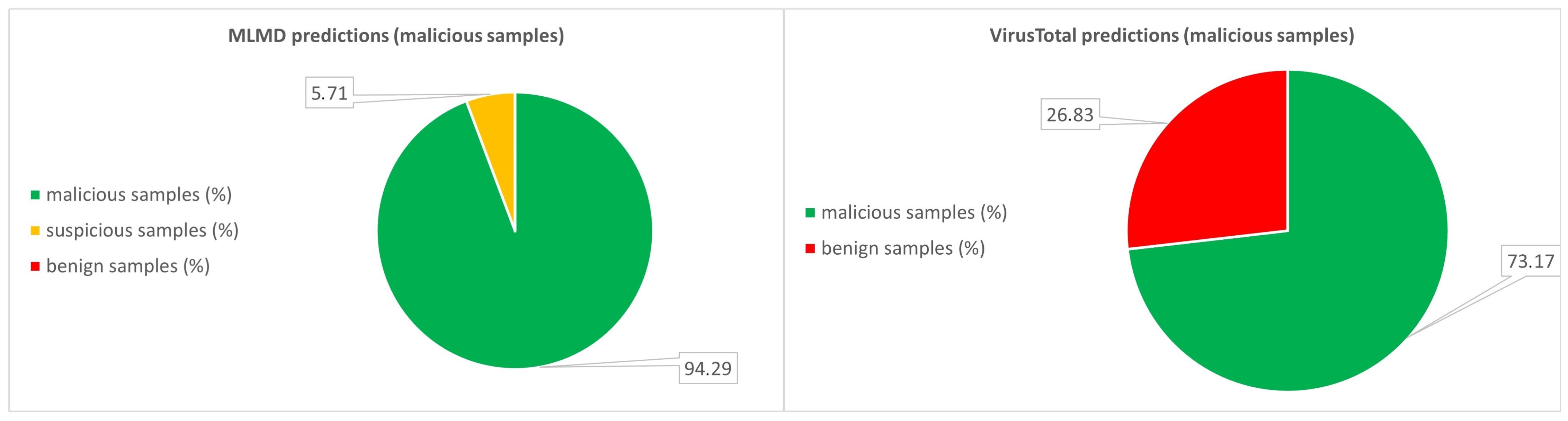
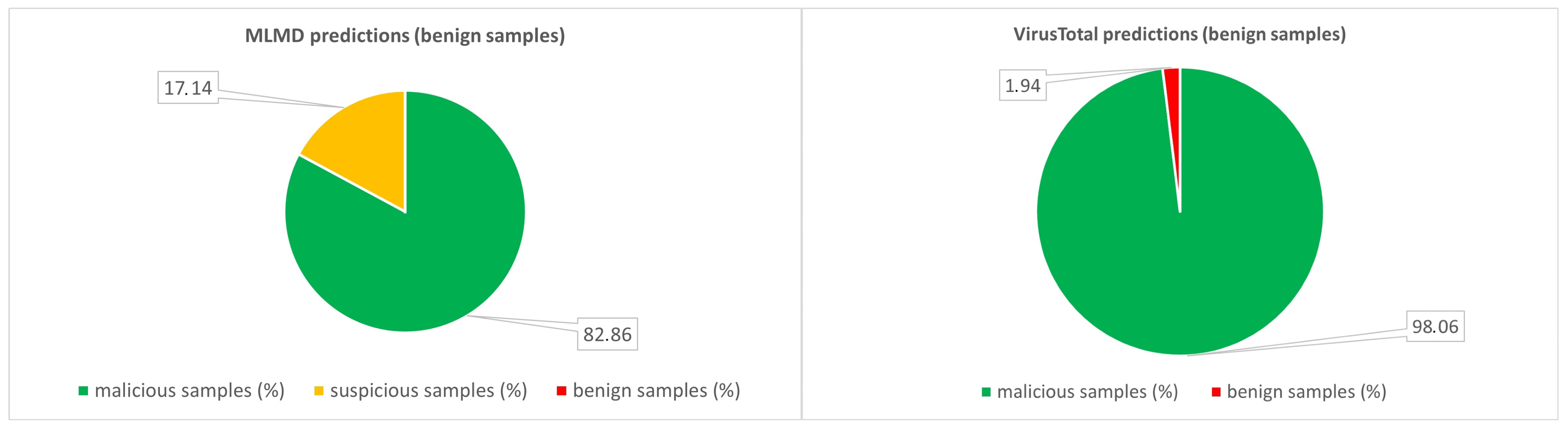
4.2.2. Comparison of Classifications

Table 17. Comparison of classifications of malicious samples.

	MLMD	VirusTotal
All samples	70	70
Malicious samples (%)	94.29	71.17
Suspicious samples (%)	5.71	-
Benign samples (%)	0	26.83

and the charts shown in Figure 11 show the percentage distribution of classifications made by our program and VirusTotal on malicious samples.

As is evident, our MLMD program classified 94.29% of all samples as malicious, which was a correct classification. The remaining 5.71% were samples classified as suspicious, which can also be considered as a partially correct answer, considering the malicious samples.

As far as VirusTotal is concerned, a total of 71.17% of systems considered the samples to be malicious. This value represents the sensitivity of VirusTotal as a whole service, not individual scanners. However, a number of systems incorrectly flagged the samples to be benign, in 26.83% of all cases.

Table 18. Comparison of classifications of benign samples.

	MLMD	VirusTotal
All samples	35	35
Malicious samples (%)	0	1.94
Suspicious samples (%)	17.14	-
Benign samples (%)	82.86	98.06

and the charts shown in Figure 12 show the percentage distribution of classifications made by our own MLMD and VirusTotal on benign samples.

As far as the benign samples are concerned, the only correct classification of the sample is its classification as benign. Our MLMD program classified 82.86% of all samples as benign, which was a correct classification. It made an incorrect classification for 17.14% of the samples (it classified the samples to be suspicious); thus, one of our classification models made an incorrect classification. However, none of the samples were classified to be malicious by the program.

The VirusTotal system—to be precise, the systems it uses—performed better on benign samples. In the case of benign samples, 98.06% of all systems correctly labelled the samples as benign and only 1.94% incorrectly as malicious.

Table 19. Number of samples classified incorrectly to be malicious samples.

Tool	Count
VirusTotal	8
MLMD	2

shows the number of samples incorrectly classified as malicious. We defined the success threshold to be 35, which is approximately half of VirusTotal’s available detection systems. Thus, this is the number of samples that were flagged correctly as malicious by fewer than 35 systems and flagged incorrectly as benign by most systems. We found eight such samples. However, our program classified only two of these samples incorrectly (i.e., as suspicious but not malicious).

A similar comparison for benign samples can be seen in

Table 20. Number of samples classified incorrectly as benign.

Tool	Count
VirusTotal	0
MLMD	6

. As in the previous case, we have defined the success threshold to be 35. Thus, the table shows the number of samples that were flagged correctly as benign by fewer than 35 systems and flagged incorrectly as malicious by most systems. However, considering VirusTotal, there were no such samples; the majority of samples was correctly detected to be benign by most systems. Our program flagged six samples as suspicious incorrectly.

In all of the above comparisons, we saw a good success rate of the XGBoost algorithm, especially in classifying the selected group of malicious samples, which confirms the success observed on the test data. However, it is important to mention that all decision-tree-based algorithms proved to be the best in detecting malware, outperforming other algorithms by a wide margin.

5. Conclusions

Our research aimed to contribute to the field of malware detection and to come up with a new solution that can help to avoid cyber threats. This led us to use machine learning algorithms and classification models, from which we evaluated the best results.

Two machine learning algorithms have been implemented, which led to the creation of classification models.

As revealed by the comparison of trained models, the best results were achieved by the XGBoost algorithm, where in the case of static analysis we achieved results with a classification accuracy of 91.92%, and in the case of dynamic analysis we achieved results with a classification accuracy of 96.48%.

The results show that the use of machine learning algorithms is sufficient to detect malware, as indicated by the existing work mentioned in the introduction to this article. Based on our experiments, we can confirm that machine learning using combined static and dynamic analysis techniques is a suitable way to detect malicious software.

Our research also includes the MLMD software, which points to the applicability of machine learning models in practice. The solution was tested against real working antivirus software with comparable results.

References

1. Monnappa, K. Learning Malware Analysis, 1st ed.; Packt Publishing: Birmingham, UK, 2018; Chapter 1; ISBN 978-178-839-250-1. [Google Scholar]
2. 2020 State of Malware Report. Available online: https://www.malwarebytes.com/resources/files/2020/02/2020_state-of-malware-report.pdf (accessed on 28 March 2022).
3. Elisan, C. Malware, Rootkits & Botnets A Beginner’s Guide, 1st ed.; McGraw-Hill Education: New York, NY, USA, 2012; Chapter 1; ISBN 978-007-179-206-6. [Google Scholar]
4. Ławrynowicz, A.; Tresp, V. Introducing Machine Learning. In Perspectives on Ontology Learning; Microsoft Press: Redmond, WA, USA, 2014; pp. 35–50. [Google Scholar]
5. Deep Instinct Website. Available online: https://www.deepinstinct.com (accessed on 10 June 2022).
6. Mohanta, A.; Saldanha, A. Malware Analysis and Detection Engineering: A Comprehensive Approach to Detect and Analyze Modern Malware, 1st ed.; Apress: New York, NY, USA, 2020; ISBN 978-148-426-192-7. [Google Scholar]
7. Fedak, A.; Stulrajter, J. Fundamentals of static malware analysis: Principles, methods, and tools. Sci. Mil. 2014, 15, 45–53. [Google Scholar]
8. Hisham, S.G. Behavior-based features model for malware detection. J. Comput. Virol. Hacking Tech. 2015, 12, 59–67. [Google Scholar]
9. Damodaran, A.; Troia, F.D.; Visaggio, C.A.; Austin, T.H.; Stamp, M. A comparison of static, dynamic, and hybrid analysis for malware detection. J. Comput. Virol. Hacking Tech. 2017, 13, 1–12. [Google Scholar] [CrossRef]
10. Cisar, P.; Joksimovic, D. Heuristic scanning and sandbox approach in malware detection. Archibald Reiss Days 2019, 9, 299–308. [Google Scholar]
11. Advanced Heuristics to Detect Zero-Day Attacks. Available online: https://hackernoon.com/advanced-heuristics-to-detect-zero-day-attacks-8e3335lt (accessed on 28 March 2022).
12. Gibert, D.; Mateu, C.; Planes, J. The rise of machine learning for detection and classification of malware: Research developments, trends and challenges. J. Netw. Comput. Appl. 2020, 153, 102526. [Google Scholar] [CrossRef]
13. Senanayake, J.; Kalutarage, H.; Al-Kadri, M.O. Android Mobile Malware Detection Using Machine Learning: A Systematic Review. Electronics 2021, 10, 1606. [Google Scholar] [CrossRef]
14. Schultz, G.M.; Eskin, E.; Zadok, F.; Stolfo, J.S. Data Mining Methods for Detection of New Malicious Executables. In Proceedings of the IEEE Computer Society Symposium on Research in Security and Privacy, Oakland, CA, USA, 13–16 May 2001; pp. 38–49. [Google Scholar]
15. Bai, J.; Wang, J.; Zou, G. A Malware Detection Scheme Based on Mining Format Information. Sci. World J. 2014, 2014, 260905. [Google Scholar] [CrossRef] [PubMed]
16. Kumar, A.; Kuppusamy, K.S.; Aghila, G. A learning model to detect maliciousness of portable executable using integrated feature set. J. King Saud Univ.—Comput. Inf. Sci. 2019, 31, 252–265. [Google Scholar] [CrossRef]
17. Bragen, R.S. Malware Detection Through Opcode Sequence Analysis Using Machine Learning. Master’s Thesis, Gjøvik University College, Gjøvik, Norway, 2015. [Google Scholar]
18. Chowdhury, M.; Rahman, A.; Islam, M. Protecting data from malware threats using machine learning technique. In Proceedings of the 2017 12th IEEE Conference on Industrial Electronics and Applications (ICIEA), Siem Reap, Cambodia, 18–20 June 2017; pp. 1691–1694. [Google Scholar]
19. Moser, A.; Kruegel, C.; Kirda, E. Limits of Static Analysis for Malware Detection. In Proceedings of the Twenty-Third Annual Computer Security Applications Conference (ACSAC 2007), Miami Beach, FL, USA, 10–14 December 2007; pp. 421–430. [Google Scholar]
20. Shijo, P.V.; Salim, A. Integrated Static and Dynamic Analysis for Malware Detection. Procedia Comput. Sci. 2015, 46, 804–811. [Google Scholar] [CrossRef] [Green Version]
21. Firdausi, I.; Lim, C.; Erwin, A.; Nugroho, A.S. Analysis of machine learning techniques used in behavior-based malware detec. In Proceedings of the 2010 Second International Conference on Advances in Computing, Control, and Telecommunication Technologies, Jakarta, Indonesia, 2–3 December 2010; pp. 201–203. [Google Scholar]
22. Mosli, R.; Yuan, B.; Li, R.; Pan, Y. A Behavior-Based Approach for Malware Detection. In Proceedings of the 13th IFIP International Conference on Digital Forensics (DigitalForensics), Orlando, FL, USA, 30 January–1 February 2017; pp. 187–201. [Google Scholar]
23. Kumar, R.; Geetha, S. Malware classification using XGboost-Gradient Boosted Decision Tree. Adv. Sci. Technol. Eng. Syst. J. 2020, 5, 536–549. [Google Scholar] [CrossRef]
24. Dhamija, H.; Dhamija, A.K. Malware Detection using Machine Learning Classification Algorithms. Int. J. Comput. Intell. Res. 2021, 17, 1–7. [Google Scholar]
25. Shhadata, I.; Bataineh, B.; Hayajneh, A.; Al-Sharif, Z.A. The Use of Machine Learning Techniques to Advance the Detection and Classification of Unknown Malware. Procedia Comput. Sci. 2020, 170, 917–922. [Google Scholar] [CrossRef]
26. VirusShare Malware Repository. Available online: https://virusshare.com/ (accessed on 29 March 2022).
27. The Portable Freeware Collection. Available online: https://www.portablefreeware.com/ (accessed on 29 March 2022).
28. Portable Software Repository. Available online: https://portableapps.com/ (accessed on 29 March 2022).
29. Dependency Walker Website. Available online: https://www.dependencywalker.com/ (accessed on 29 March 2022).
30. Cuckoo Sandbox Website. Available online: https://cuckoosandbox.org/ (accessed on 29 March 2022).
31. Hossin, M.; Sulaiman, M.N. A Review on Evaluation Metrics for Data Classification Evaluations. Int. J. Data Min. Knowl. Manag. Process 2015, 5, 1–11. [Google Scholar]
32. Sutorčík, K. Detection of Malware Samples Using Machine Learning Algorithms and Methods of Dynamic Analysis (In Orig Lang: Využitie Algoritmov StrojovéHo UčEnia na Detekciu MalvéRovýCh Vzoriek Pomocou MetóD Dynamickej Analýzy). Master’s Thesis, Technická Univerzita v Košiciach, Košice, Slovakia, 2021. [Google Scholar]
33. Špakovský, E. Detection of Malware Samples Using Machine Learning Algorithms and Methods of Static Analysis (In Orig Lang: Využitie Algoritmov StrojovéHo UčEnia na Detekciu MalvéRovýCh Vzoriek Pomocou MetóD Statickej Analýzy). Master’s Thesis, Technická Univerzita v Košiciach, Košice, Slovakia, 2021. [Google Scholar]
Figure 1. Static analysis output (excerpt).
Applsci 12 06672 g001
Figure 2. Architecture of the dynamic analysis environment.
Applsci 12 06672 g002
Figure 3. Dynamic analysis output.
Applsci 12 06672 g003
Figure 4. The confusion matrix.
Applsci 12 06672 g004
Figure 5. ROC for the best models: (a) ROC for XGB_S_1 model; (b) ROC for XGB_D_1 model.
Applsci 12 06672 g005
Figure 6. The main screen of the program.
Applsci 12 06672 g006
Figure 7. The proposed detection method.
Applsci 12 06672 g007
Figure 8. Action on a scanned file.
Applsci 12 06672 g008
Figure 9. Output after URL analysis by Cuckoo Sandbox.
Applsci 12 06672 g009
Figure 10. The quarantine screen.
Applsci 12 06672 g010
Figure 11. Comparison of predictions of malicious samples.
Applsci 12 06672 g011
Figure 12. Comparison of classifications of malicious samples.
Applsci 12 06672 g012