
Shaping and Dilating the Fitness Landscape for Parameter Estimation in Stochastic Biochemical Models

 ,
,  , , and
Abstract
:Featured Application
Abstract
1. Introduction
2. Materials and Methods
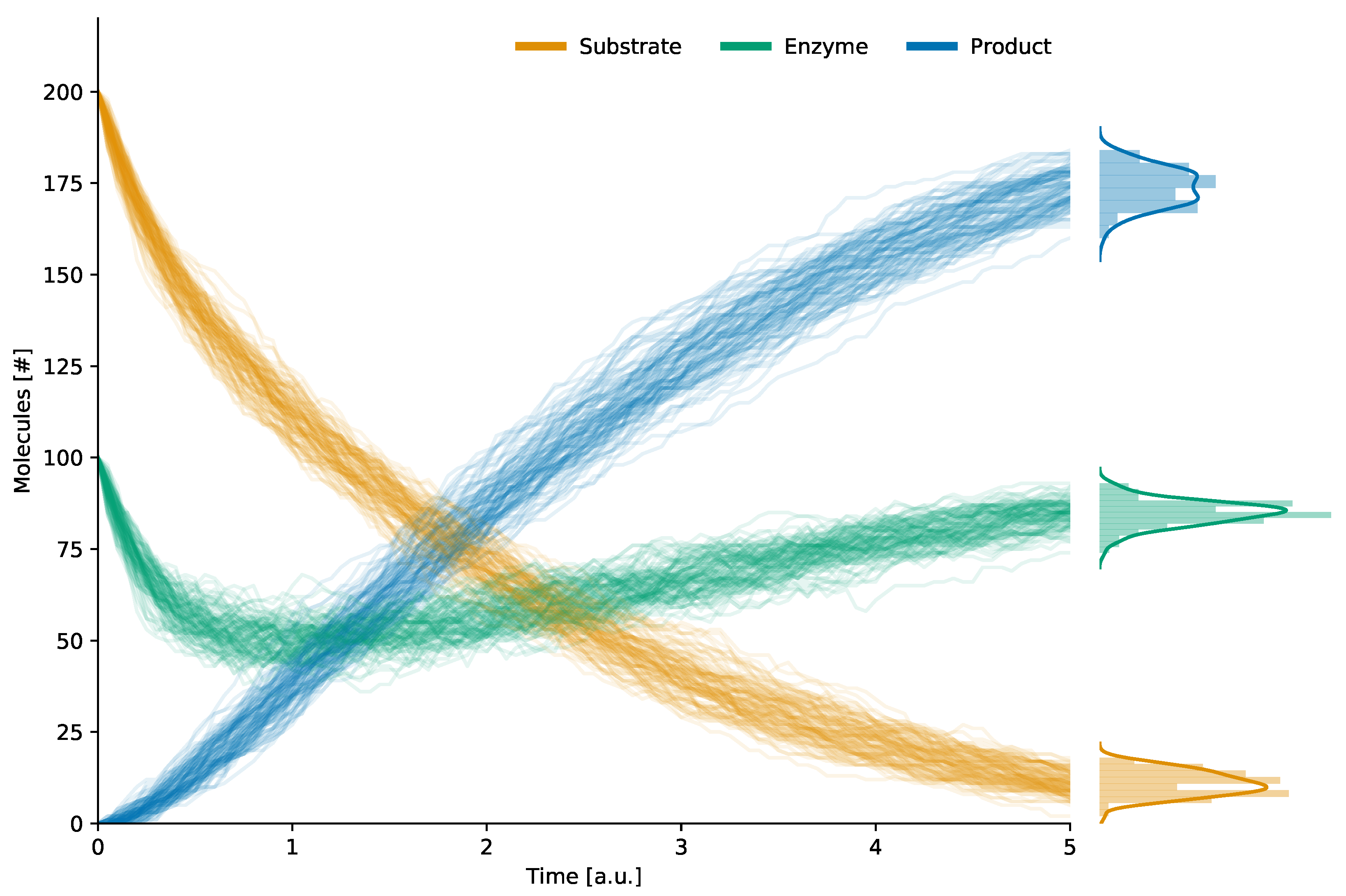
2.1. Reaction-Based Modeling and Stochastic Simulation Algorithm
- The set of molecular species;
- The set of the biochemical reactions describing all interactions among the species in .
- ;
- ;
- .
2.2. Fuzzy Self-Tuning Particle Swarm Optimization
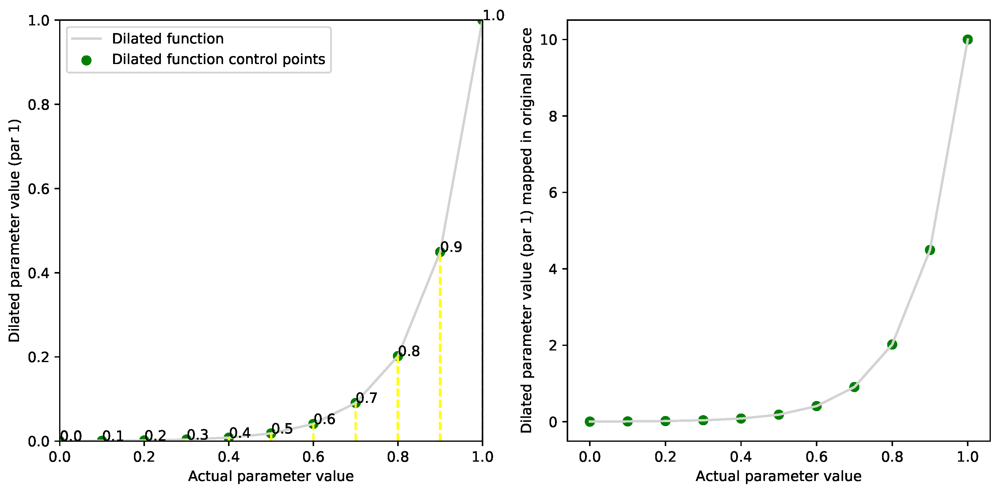
2.3. Dilation Functions
2.4. Evolving Dilation Functions
2.5. Surrogate Fourier Modeling with surF
- 1.
- Discrete Cosine Transform.
- 2.
- Reducing the number of samples.
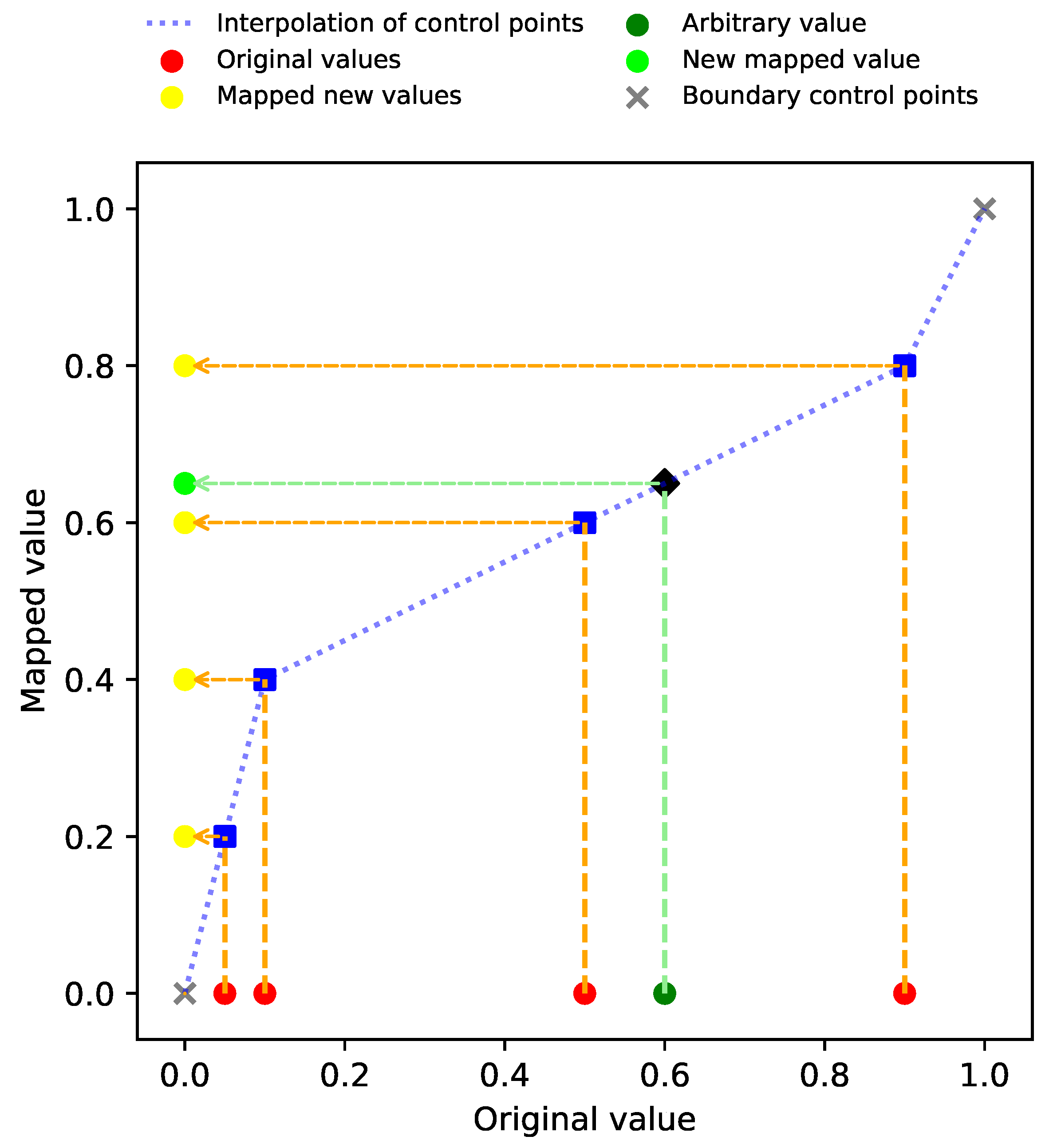
- If is in the convex hull defined by the points , then is obtained by a linear interpolation;
- otherwise, a linear interpolation is not possible and is defined as , where is the point among nearest to .
- 3.
- Parameters of surF.
- , which is the number of samples from f used to build ;
- , which is the “density” of samples from to obtain the points used to calculate the DFT; and
- , which controls the number of low frequencies preserved.
3. Results
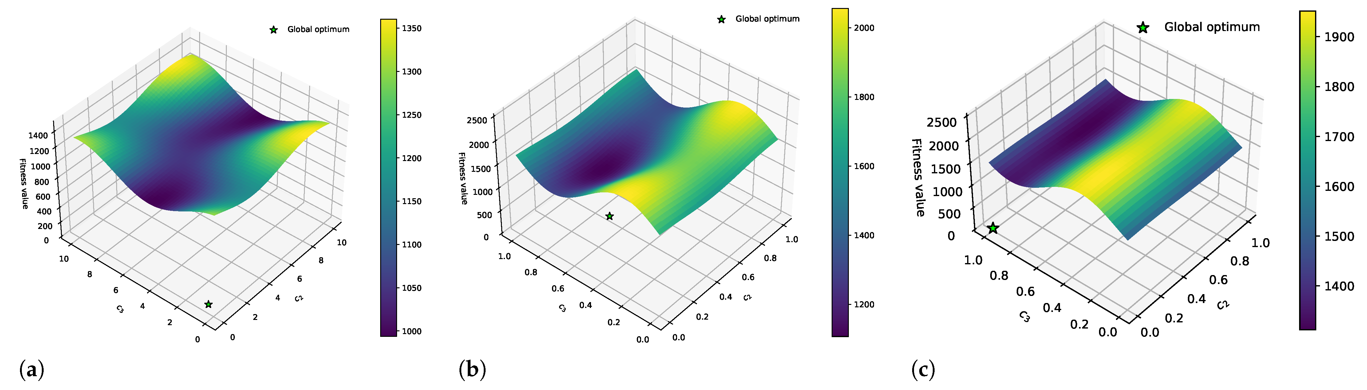
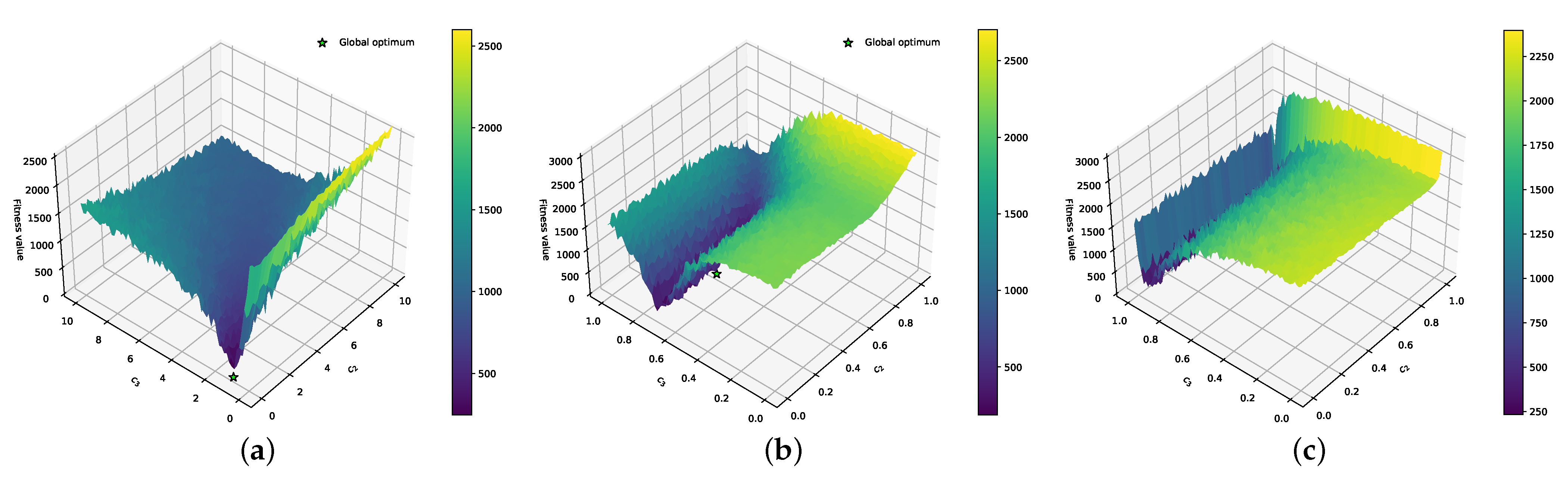
3.1. Effect of DFs on the PE Problem
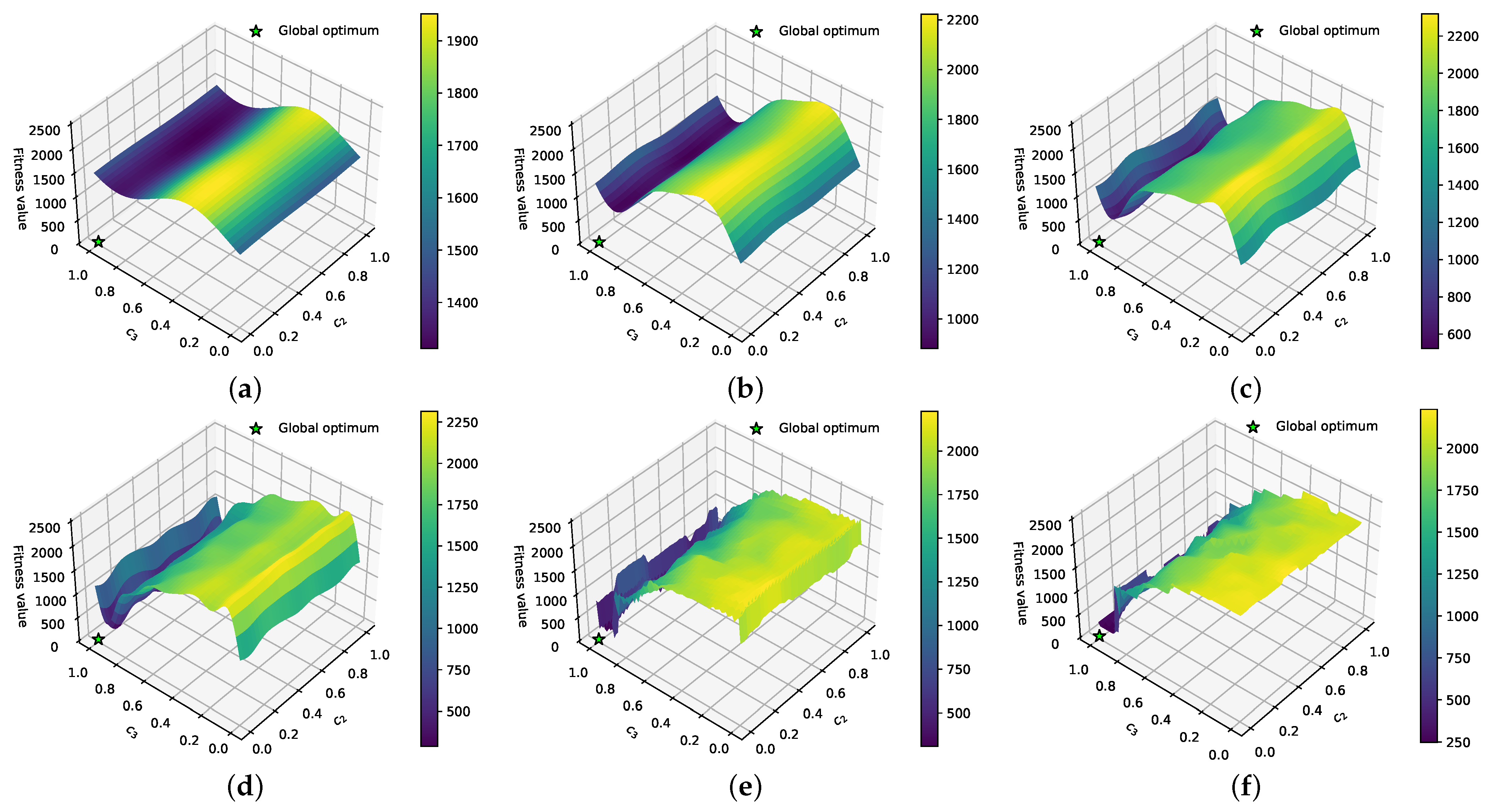
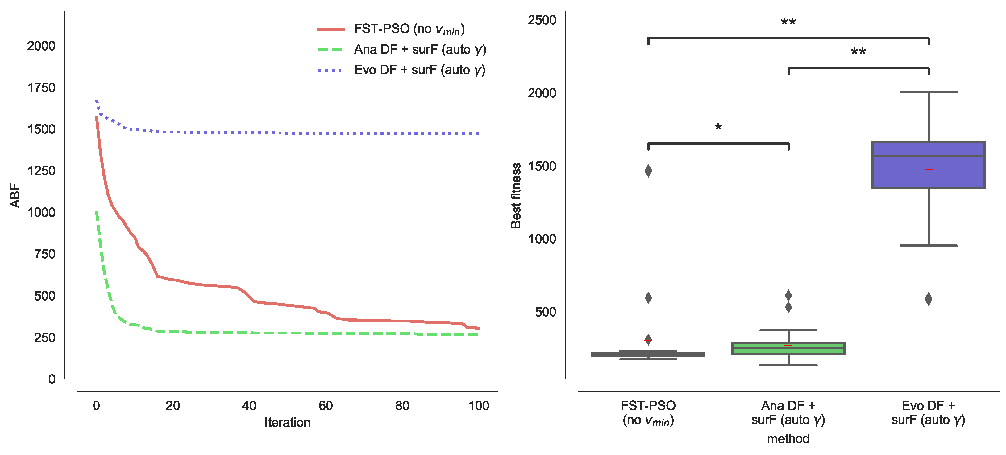
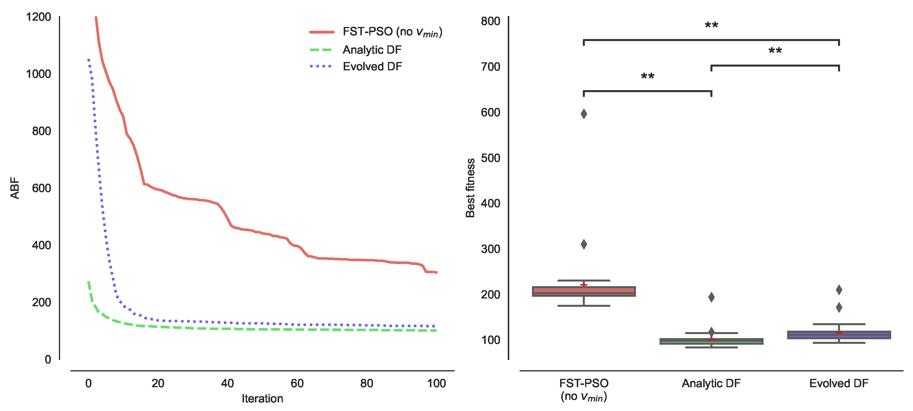
3.2. Combining DFs and Fourier Surrogate Modeling
4. Discussion
Author Contributions
Funding
Institutional Review Board Statement
Informed Consent Statement
Data Availability Statement
Conflicts of Interest
Abbreviations
| ABF | Average Best Fitness |
| BF | Basis Function |
| DCT | Discrete Cosine Transform |
| DF | Dilation Function |
| E | Enzyme |
| ES | Enzyme–Substrate complex |
| FRBS | Fuzzy Rule-Based System |
| FST-PSO | Fuzzy Self-Tuning Particle Swarm Optimization |
| MM | Michaelis–Menten |
| P | Product |
| PE | Parameter Estimation |
| PSO | Particle Swarm Optimization |
| RBM | Reaction-Based Model |
| S | Substrate |
| SSA | Stochastic Simulation Algorithm |
| surF | Fitness Landscape Surrogate Modeling with Fourier Filtering |
| Mathematical Notation | |
| stoichiometric coefficients associated with the n-th reactant | |
| stoichiometric coefficients associated with the m-th reaction | |
| vector of stochastic constants | |
| stochastic (kinetic) constant | |
| cognitive attractor of FST-PSO | |
| social attractor of FST-PSO | |
| D | number of dimensions of the search space |
| number of distinct combinations of the reactant molecules | |
| f | original fitness function |
| dilated fitness function | |
| , | surrogate fitness functions |
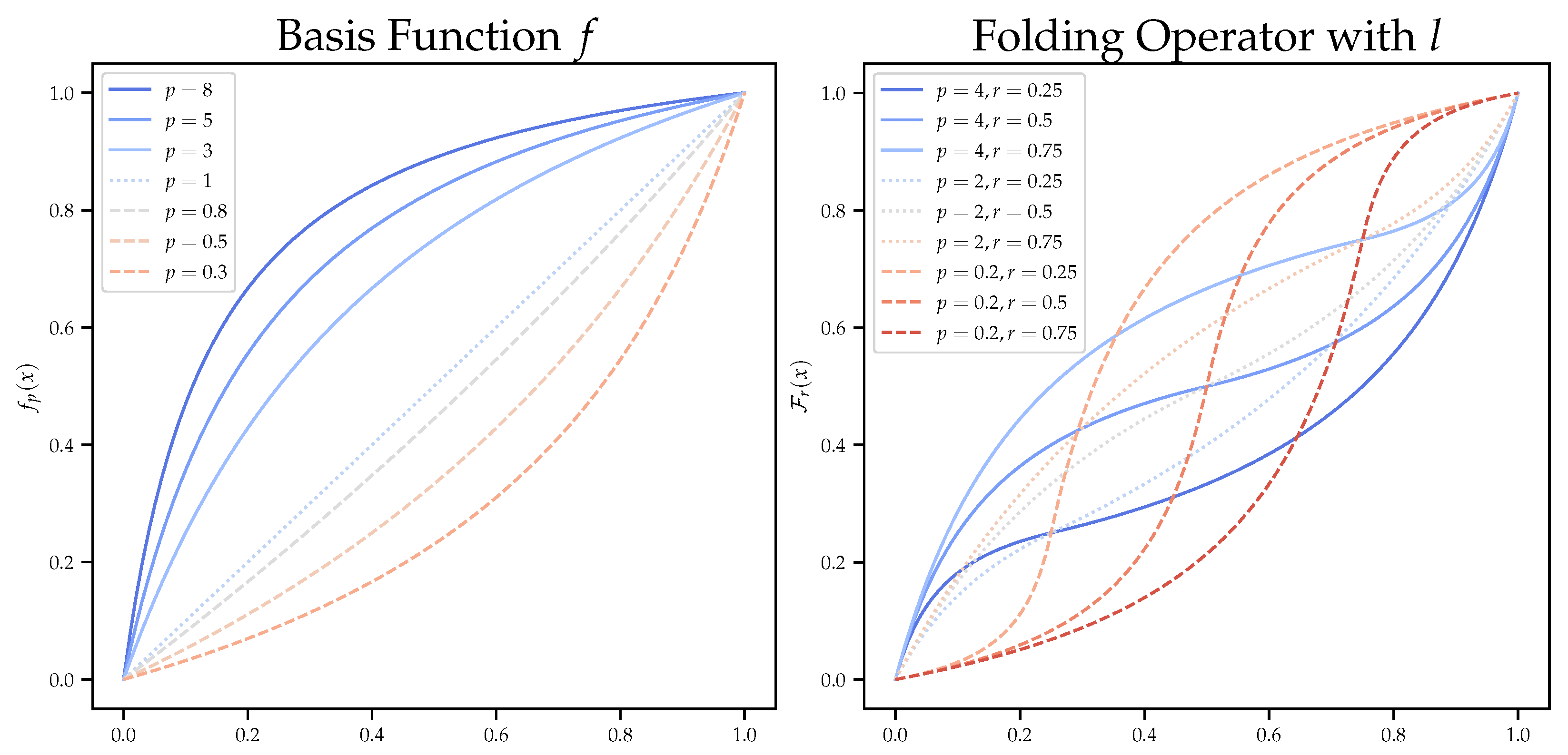
| folding operator | |
| number of lower frequencies to not be zeroed | |
| I | number of sampled points to compute the dilated landscape |
| lower and upper bounds of the search space | |
| linear basis function | |
| the experimental (target) amount of measured at time | |
| p | parameter of the linear basis function |
| coefficient representing the amplitude of -th frequency | |
| r | parameter of the folding operator |
| set of biochemical reactions | |
| m-th biochemical reaction | |
| number of equally spaced points to build the surrogate function | |
| set of molecular species | |
| i-th molecular specie | |
| number of samples used to construct the surrogate | |
| t | time of the system |
| vector of time points | |
| k-th time point | |
| waiting time | |
| maximum velocity of the FST-PSO particles | |
| minimum velocity of the FST-PSO particles | |
| inertia factor of FST-PSO | |
| simulated amount of the species at time | |
| vector representing the state of the system at time t | |
| amount of the n-th molecular specie | |
| control point | |
| Q-th control point | |
| length of the individuals representing the DFs | |
| vector of control points | |
| fitness value of the -th point of the surrogate | |
| -th point of the search space to build the surrogate function | |
| random number sampled from an uniform distribution | |
| random number sampled from an uniform distribution |
References
- Munsky, B.; Tuzman, K.T.; Fey, D.; Dobrzynski, M.; Kholodenko, B.N.; Olson, S.; Huang, J.; Fox, Z.; Singh, A.; Grima, R.; et al. Quantitative Biology: Theory, Computational Methods, and Models; The MIT Press: Cambridge, MA, USA, 2018. [Google Scholar]
- Nobile, M.S.; Besozzi, D.; Cazzaniga, P.; Mauri, G.; Pescini, D. A GPU-based multi-swarm PSO method for parameter estimation in stochastic biological systems exploiting discrete-time target series. In Evolutionary Computation, Machine Learning and Data Mining in Bioinformatics; LNCS; Giacobini, M., Vanneschi, L., Bush, W., Eds.; Springer: Berlin/Heidelberg, Germany, 2012; Volume 7246, pp. 74–85. [Google Scholar]
- Nobile, M.S.; Besozzi, D.; Cazzaniga, P.; Mauri, G.; Pescini, D. Estimating reaction constants in stochastic biological systems with a multi-swarm PSO running on GPUs. In Proceedings of the 14th Annual Conference companion on Genetic and Evolutionary Computation (ACM 2012), New York, NY, USA, 7–11 July 2012; pp. 1421–1422. [Google Scholar]
- Daigle, B.J.; Roh, M.K.; Petzold, L.R.; Niemi, J. Accelerated maximum likelihood parameter estimation for stochastic biochemical systems. BMC Bioinform. 2012, 13, 68. [Google Scholar] [CrossRef] [PubMed] [Green Version]
- Nobile, M.S.; Cazzaniga, P.; Spolaor, S.; Besozzi, D.; Manzoni, L. Fourier Surrogate Models of Dilated Fitness Landscapes in Systems Biology: Or how we learned to torture optimization problems until they confess. In Proceedings of the 2020 IEEE Conference on Computational Intelligence in Bioinformatics and Computational Biology (CIBCB), Via del Mar, Chile, 27–29 October 2020; pp. 1–8. [Google Scholar]
- Nobile, M.S.; Cazzaniga, P.; Ashlock, D.A. Dilation Functions in Global Optimization. In Proceedings of the 2019 IEEE Congress on Evolutionary Computation (CEC), Wellington, New Zealand, 10–13 June 2019; pp. 2300–2307. [Google Scholar]
- Chunming, F.; Yadong, X.; Jiang, C.; Xu, H.; Huang, Z. Improved differential evolution with shrinking space technique for constrained optimization. Chin. J. Mech. Eng. 2017, 30, 553–565. [Google Scholar]
- Wang, Y.; Cai, Z.; Zhou, Y. Accelerating adaptive trade-off model using shrinking space technique for constrained evolutionary optimization. Int. J. Numer. Methods Eng. 2009, 77, 1501–1534. [Google Scholar] [CrossRef]
- Aguirre, A.H.; Rionda, S.B.; Coello Coello, C.A.; Lizárraga, G.L.; Montes, E.M. Handling constraints using multiobjective optimization concepts. Int. J. Numer. Methods Eng. 2004, 59, 1989–2017. [Google Scholar] [CrossRef]
- Wang, H.; Wu, Z.; Liu, Y.; Wang, J.; Jiang, D.; Chen, L. Space transformation search: A new evolutionary technique. In Proceedings of the First ACM/SIGEVO Summit on Genetic and Evolutionary Computation (ACM 2009), New York, NY, USA, 12–14 June 2009; pp. 537–544. [Google Scholar]
- Bhosekar, A.; Ierapetritou, M. Advances in surrogate based modeling, feasibility analysis, and optimization: A review. Comput. Chem. Eng. 2018, 108, 250–267. [Google Scholar] [CrossRef]
- Manzoni, L.; Papetti, D.M.; Cazzaniga, P.; Spolaor, S.; Mauri, G.; Besozzi, D.; Nobile, M.S. Surfing on fitness landscapes: A boost on optimization by Fourier surrogate modeling. Entropy 2020, 22, 285. [Google Scholar] [CrossRef] [PubMed] [Green Version]
- Nobile, M.S.; Spolaor, S.; Cazzaniga, P.; Papetti, D.M.; Besozzi, D.; Ashlock, D.A.; Manzoni, L. Which random is the best random? A study on sampling methods in Fourier surrogate modeling. In Proceedings of the 2020 IEEE Congress on Evolutionary Computation (CEC), Glasgow, UK, 19–24 July 2020. [Google Scholar]
- Nobile, M.S.; Cazzaniga, P.; Besozzi, D.; Colombo, R.; Mauri, G.; Pasi, G. Fuzzy Self-Tuning PSO: A settings-free algorithm for global optimization. Swarm Evol. Comput. 2018, 39, 70–85. [Google Scholar] [CrossRef]
- Poli, R.; Kennedy, J.; Blackwell, T. Particle swarm optimization. Swarm Intell. 2007, 1, 33–57. [Google Scholar] [CrossRef]
- Gillespie, D.T. Exact stochastic simulation of coupled chemical reactions. J. Phys. Chem. 1977, 81, 2340–2361. [Google Scholar] [CrossRef]
- Cazzaniga, P.; Damiani, C.; Besozzi, D.; Colombo, R.; Nobile, M.S.; Gaglio, D.; Pescini, D.; Molinari, S.; Mauri, G.; Alberghina, L.; et al. Computational strategies for a system-level understanding of metabolism. Metabolites 2014, 4, 1034–1087. [Google Scholar] [CrossRef] [PubMed]
- Elowitz, M.B.; Levine, A.J.; Siggia, E.D.; Swain, P.S. Stochastic gene expression in a single cell. Science 2002, 297, 1183–1186. [Google Scholar] [CrossRef] [PubMed] [Green Version]
- Nobile, M.S.; Tangherloni, A.; Rundo, L.; Spolaor, S.; Besozzi, D.; Mauri, G.; Cazzaniga, P. Computational Intelligence for Parameter Estimation of Biochemical Systems. In Proceedings of the 2018 IEEE Congress on Evolutionary Computation (CEC), Rio de Janeiro, Brazil, 8–13 July 2018; pp. 1–8. [Google Scholar]
- Nelson, D.; Cox, M. Lehninger Principles of Biochemistry; W. H. Freeman Company: New York, NY, USA, 2004. [Google Scholar]
- Empereur-Mot, C.; Pesce, L.; Doni, G.; Bochicchio, D.; Capelli, R.; Perego, C.; Pavan, G.M. Swarm-CG: Automatic Parametrization of Bonded Terms in MARTINI-Based Coarse-Grained Models of Simple to Complex Molecules via Fuzzy Self-Tuning Particle Swarm Optimization. ACS Omega 2020, 5, 32823–32843. [Google Scholar] [CrossRef]
- Tangherloni, A.; Spolaor, S.; Cazzaniga, P.; Besozzi, D.; Rundo, L.; Mauri, G.; Nobile, M.S. Biochemical parameter estimation vs. benchmark functions: A comparative study of optimization performance and representation design. Appl. Soft Comput. 2019, 81, 105494. [Google Scholar] [CrossRef]
- SoltaniMoghadam, S.; Tatar, M.; Komeazi, A. An improved 1-D crustal velocity model for the Central Alborz (Iran) using Particle Swarm Optimization algorithm. Phys. Earth Planet. Inter. 2019, 292, 87–99. [Google Scholar] [CrossRef]
- Fuchs, C.; Spolaor, S.; Nobile, M.S.; Kaymak, U. A Swarm Intelligence Approach to Avoid Local Optima in Fuzzy C-Means Clustering. In Proceedings of the 2019 IEEE International Conference on Fuzzy Systems (FUZZ-IEEE), New Orleans, LA, USA, 23–26 June 2019; pp. 1–6. [Google Scholar]
- Papetti, D.M.; Ashlock, D.A.; Cazzaniga, P.; Besozzi, D.; Nobile, M.S. If You Can’t Beat It, Squash It: Simplify Global Optimization by Evolving Dilation Functions. In Proceedings of the 2021 IEEE Congress on Evolutionary Computation (CEC), Kraków, Poland, 28 June–1 July 2021. [Google Scholar]
- Cazzaniga, P.; Nobile, M.S.; Besozzi, D. The impact of particles initialization in PSO: Parameter estimation as a case in point. In Proceedings of the 2015 IEEE Conference on Computational Intelligence in Bioinformatics and Computational Biology (CIBCB), Niagara Falls, ON, Canada, 12–15 August 2015; pp. 1–8. [Google Scholar]
- Beyer, H.G.; Schwefel, H.P. Evolution strategies—A comprehensive introduction. Nat. Comput. 2002, 1, 3–52. [Google Scholar] [CrossRef]
- Cooley, J.W.; Tukey, J.W. An algorithm for the machine calculation of complex Fourier series. Math. Comput. 1965, 19, 297–301. [Google Scholar] [CrossRef]
- Sobol’, I.M. On the distribution of points in a cube and the approximate evaluation of integrals. Zhurnal Vychislitel’noi Mat. I Mat. Fiz. 1967, 7, 784–802. [Google Scholar] [CrossRef]
- Spolaor, S.; Gribaudo, M.; Iacono, M.; Kadavy, T.; Oplatková, Z.K.; Mauri, G.; Pllana, S.; Senkerik, R.; Stojanovic, N.; Turunen, E.; et al. Towards Human Cell Simulation. In High-Performance Modelling and Simulation for Big Data Applications; Lecture Notes in Computer Science; Springer: Berlin/Heidelberg, Germany, 2019; Volume 11400, pp. 221–249. [Google Scholar]


| Molecular Species | Amount |
|---|---|
| S (substrate) | 200 |
| E (enzyme) | 100 |
| (enzyme–substrate complex) | 0 |
| P (product) | 0 |
| ID | Name | Semantics |
|---|---|---|
| 0 | Identity | |
| 1 | Linear transformation | |
| 2 | ||
| 3 | Folding operators | |
| 4 |
Publisher’s Note: MDPI stays neutral with regard to jurisdictional claims in published maps and institutional affiliations. |
© 2022 by the authors. Licensee MDPI, Basel, Switzerland. This article is an open access article distributed under the terms and conditions of the Creative Commons Attribution (CC BY) license (https://creativecommons.org/licenses/by/4.0/).
Share and Cite
Nobile, M.S.; Papetti, D.M.; Spolaor, S.; Cazzaniga, P.; Manzoni, L. Shaping and Dilating the Fitness Landscape for Parameter Estimation in Stochastic Biochemical Models. Appl. Sci. 2022, 12, 6671. https://doi.org/10.3390/app12136671
Nobile MS, Papetti DM, Spolaor S, Cazzaniga P, Manzoni L. Shaping and Dilating the Fitness Landscape for Parameter Estimation in Stochastic Biochemical Models. Applied Sciences. 2022; 12(13):6671. https://doi.org/10.3390/app12136671
Chicago/Turabian StyleNobile, Marco S., Daniele M. Papetti, Simone Spolaor, Paolo Cazzaniga, and Luca Manzoni. 2022. "Shaping and Dilating the Fitness Landscape for Parameter Estimation in Stochastic Biochemical Models" Applied Sciences 12, no. 13: 6671. https://doi.org/10.3390/app12136671
APA StyleNobile, M. S., Papetti, D. M., Spolaor, S., Cazzaniga, P., & Manzoni, L. (2022). Shaping and Dilating the Fitness Landscape for Parameter Estimation in Stochastic Biochemical Models. Applied Sciences, 12(13), 6671. https://doi.org/10.3390/app12136671