A Switched Variational Estimation Algorithm for Continuous Discrete Measurement Information Loss in Underwater Navigation: Linear versus Nonlinear

Abstract

In various applications of automatic underwater vehicles (AUVs), it is necessary to acquire the real-time location and speed information of the AUV. However, the complicated and fluctuating marine environment leads to measurement information loss. The accuracy of noise measurement is vital for accurate state estimation, but it is difficult for traditional algorithms to acquire time-varying noise measurements. Due to inaccurate process models and measurement noise, the filtering performance becomes poor or even diverges. To address the problems above, a switched variational estimation filtering (SVEF) algorithm, which combines the advantages of both Gaussian filtering and the variational estimation (VE) method, is proposed. In SVEF, VE is embedded into a linear or nonlinear filtering algorithm. Owing to the continuous discrete underwater navigation model, the state vector is estimated by the SVEF in the case of measurement information loss, and the accurate position and velocity of the AUV are determined. The experimental results prove that the SVEF achieves better positioning precision and is more robust than other conventional algorithms for AUV applications.

1. Introduction

Nowadays, autonomous underwater vehicles (AUVs) have been widely used by many communities for commercial, offshore, and defense applications [1]. Especially in deep-sea exploration and development, AUVs are playing significant roles [2]. This is largely due to the rapid development of underwater navigation technology. To complete predefined underwater tasks, such as surveying, underwater detection, and underwater reconnaissance, the importance of accurate position and velocity information for AUVs is increasingly being emphasized [3].

The inertial navigation system (INS) is the most widely used position- and speed-acquisition technology for underwater navigation [4]. For cost reasons, the microelectromechanical systems (MEMSs)-based inertial sensors are commonly used in AUVs. However, because of the characteristics of MEMS-based sensors, the error introduced by the INS solution increases over time. These errors can lead to a sharp drop in the positioning performance of AUVs [5]. In addition, due to the existence of various noises, such as ocean currents, salt cliffs, and surrounding ships, the marine environment is complicated and time-varying, resulting in the loss of measurement information [6,7]. To eliminate the influence of complex measurement noise and the measurement information randomly lost, several Bayesian-theory-based filtering algorithms have been proposed and applied, such as the extended Kalman filter (EKF) [8,9], unscented Kalman filter (UKF) [10], Cubature Kalman filter (CKF) [11], and so on. The performance of the filtering algorithms is crucial in judging whether the AUV can properly work and safely return [12,13,14].

EKF is the most widely used algorithm for integrating navigation signals, such as position, velocity, and so on, which can restrict the system defects and improve the calculation accuracy. However, it is well-known that the measurement and process noises of the EKF are assumed to be uncorrelated, and both are assumed to satisfy the zero-mean Gaussian distribution. Due to the presence of stochastic non-Gaussian noise, the inaccurate noise assumptions may cause velocity and position drifts. Moreover, EKF struggles to deal with the impact of system uncertainty. In recent years, many improved algorithms based on EKF have been developed, such as adaptive EKF [15], fuzzy EKF [16], iterated EKF, and so on. However, for strongly nonlinear systems, the truncation error, caused by the Taylor-series expansion-based linearization process [17,18,19], leads to serious degradation of filter performance.

To overcome the influence of truncation error, improved UKF-algorithm-based unscented transformation and UKF-based algorithms are proposed as maximum correlation entropy-based UKF and adaptive UKF, respectively [20,21,22]. For MEMS-grade INS, UKF is more adaptable to highly nonlinear models than EKF [23,24]. Similar to UKF, CKF is a sigma point Gaussian approximation filter. However, unlike UKF, which is a uniform selection of 2n+1 sigma points around the expectation, the spherical cubature rule is used by the CKF to select 2n cubature points and thus estimate the mean and correlation covariance of the posterior probability density by solving for the spherical mean integral. Some CKF-based algorithms, such as embedded CKF and variational Bayesian adaptive CKF, have been proposed to achieve navigation signal integration in recent years [25,26]. When the same matrix decomposition methods, such as square root decomposition, are used for UKF and CKF, the computational burden of CKF is lower than that of UKF. Moreover, due to the insensitivity of the CKF to increases in dimension, the stability of CKF is better than that of UKF if the system has a high dimension, e.g., the dimensional order is greater than three. However, the complex marine environment can cause a loss of measurement information, so these navigation algorithms tend to diverge when working underwater and have very limited practical application effects.

In addition, it is hard to establish precise observation noise models in underwater integrated navigation models because the sensor performance changes with the environment. Therefore, the variational estimation (VE) method was introduced. The method is simple and easy, and the approximation degree increases in each iteration [27]. Unlike other optimization algorithms, there is no need for the VE method to calculate Jacobian matrices, regardless of calculating the joint probability density function (PDF) [28]. Therefore, the VE-based method is effective for obtaining accurate measurement noise. A few VE-based algorithms have been proposed, such as neural network-assisted variational Bayesian adaptive CKF [29] and the variational Bayesian adaptive cubature information filter [30]. However, in these algorithms, the influence of inaccurate process noise is ignored, and the information filter performs poorly when the state dimension is low. Although various solutions have been proposed for underwater navigation in recent years, and great progress has been made [31,32,33], the measurement information loss in underwater environments is still an open issue. In this paper, a switched variational estimation filter (SVEF) algorithm is proposed, which combines the merits of the Gaussian filter and VE method. The Gaussian filter is used to obtain a more accurate state vector information estimation, and the VE method can help with computing the optimal solution of measurement noise and with predicting the error covariance matrix and measurement loss information. The proposed SVEF algorithm has high estimation accuracy and good robustness, especially when working in ocean and marine environments for long periods of time. The major contributions are as follows:

(1)

A new method searching for the optimal solution is designed, in which the initial loss parameter makes a valuable contribution toward state estimation;

(2)

The problem of measurement information loss in a continuous discrete underwater navigation model (i.e., the state model is continuous and the measurement model is discrete) is effectively solved by the proposed SVEF algorithm;

(3)

In the VE method, linear or nonlinear filtering is employed to effectively determine the state vector; moreover, the measurement error covariance matrix and predicted error covariance matrix are accurately calculated.

The remainder of the article is presented as follows: The underwater navigation system and the preliminaries of the measurement information loss are given in Section 2. Section 3 proposes an SVEF algorithm based on the VE method, which is a novel hybrid algorithm for time-varying noise matrices. The proposed SVEF is tested and evaluated in Section 4 by using the raw data collected in real underwater experiments. Section 5 concludes the paper.

2. Problem Statement

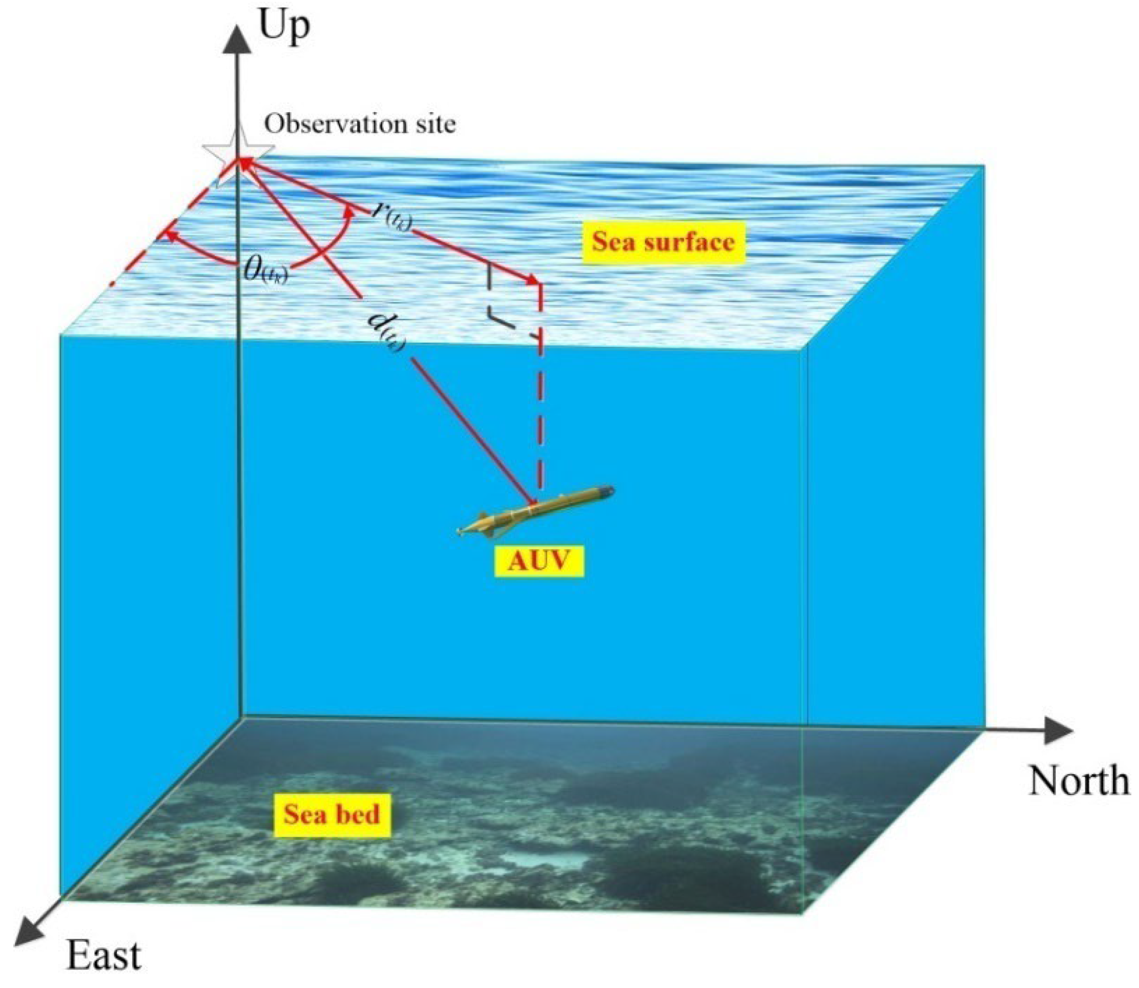
2.1. Underwater Navigation Model

The motion model of the AUV is shown in Equation (1) by using continuous process and discrete measurement equations, and the motion model of the AUV and underwater navigation system are shown in Figure 1.

$$\{\begin{array}{l}dX\left(t\right)=F\left(t\right)X\left(t\right)dt+\omega \left(t\right)dt\\ Z\left(t_k\right)=\xi \left(t_k\right)+h\left[X\left(t_k\right)\right]+v\left(t_k\right)=\xi \left(t_k\right)+H_{k}X\left(t_k\right)+v\left(t_k\right)\end{array}$$

(1)

where the state vector $X\left(t\right)={\left[\begin{array}{cccccc}{x}_t& v_{x,t}& y_t& v_{y,t}& z_t& v_{z,t}\end{array}\right]}^T$, $x_t$ and $v_{x,t}$ refer to the position and speed of the AUV in the east direction, respectively; $y_t$ and $v_{y,t}$ refer to the position and speed of the AUV in the north direction, respectively; $z_t$ and $v_{z,t}$ refer to the position and speed of the AUV in the up-direction, respectively; the subscript t indicates continuous time t; $F\left(t\right)$ represents the state transition equation; $Z\left(t_k\right)$ refers to the observation vector of discrete time k; $\omega \left(t\right)$ is the process noise obeying the Gaussian distribution with zero mean; the process noise matrix is $Q\left(t\right)$; $v\left(t_k\right)$ is the observation noise obeying the Gaussian distribution with zero mean; the observation noise matrix is $R_k$; $\xi \left(t_k\right)$ is the random variable at the discrete time k; $H_k$ and $h[•]$ are the measurement functions of linear (Case 1) and nonlinear (Case 2) forms, respectively.

Case 1: The measurement function is linear, including Case 1.1, Case 1.2, and Case 1.3.

The observation vector is denoted as follows:

$$H_{k}X\left(t_k\right)+v\left(t_k\right)={\left[\begin{array}{ccc}x\left(t_k\right)& y\left(t_k\right)& z\left(t_k\right)\end{array}\right]}^T$$

(2)

where $H_k=\left[\begin{array}{rrrrrr}\hfill 1& \hfill 0& \hfill 0& \hfill 0& \hfill 0& \hfill 0\\ \hfill 0& \hfill 0& \hfill 1& \hfill 0& \hfill 0& \hfill 0\\ \hfill 0& \hfill 0& \hfill 0& \hfill 0& \hfill 1& \hfill 0\end{array}\right]$; $x\left(t_k\right)$, $y\left(t_k\right)$, and $z\left(t_k\right)$ indicate the measured position in all directions at discrete time k.

Case 2: The measurement function is nonlinear, including Case 2.1, Case 2.2, and Case 2.3.

The observation vector is denoted as follows:

$$h\left[X\left(t_k\right)\right]+v\left(t_k\right)=\left[\begin{array}{c}\sqrt{{\left(x_t-x_0\right)}^2+{\left(y_t-y_0\right)}^2}\\ \sqrt{{\left(x_t-x_0\right)}^2+{\left(y_t-y_0\right)}^2+{\left(z_t-z_0\right)}^2}\\ \arctan \left[\frac{\left(y_t-y_0\right)}{\left(x_t-x_0\right)}\right]\end{array}\right]+v\left(t_k\right)={\left[\begin{array}{ccc}r\left(t_k\right)& d\left(t_k\right)& \theta \left(t_k\right)\end{array}\right]}^T$$

(3)

where the elements of $Z\left(t_k\right)$ are depicted in Figure 1. $x_0$, $y_0$, and $z_0$ mean the position of the observation site in all directions; $r\left(t_k\right)$ is the horizontal distance between the observation site and the AUV measured at time k; $d\left(t_k\right)$ is the three-dimensional Euclidean distance between the observation site and the AUV at time k; $\theta \left(t_k\right)$ indicates the measured angle of the AUV with respect to the observation site at discrete time k.

2.2. Preliminaries of the Measurement Information Loss

The distribution of $\xi \left(t_k\right)$ is denoted as:

$$\{\begin{array}{l}\xi \left(t_k\right)=1,\mathrm{Pro}\left[\xi \left(t_k\right)=1\right]=\tau \left(t_k\right)\\ \xi \left(t_k\right)=0,\mathrm{Pro}\left[\xi \left(t_k\right)=0\right]=\left[1-\tau \left(t_k\right)\right]\end{array}$$

(4)

where $\xi \left(t_k\right)$ satisfies the Bernoulli distribution; $\mathrm{Pro}[•]$ denotes the PDF; $\tau \left(t_k\right)$ is the acquisition probability at the discrete time k; $\left[\xi \left(t_k\right)=1\right]$ indicates that the observation vector was successfully measured; $\left[\xi \left(t_k\right)=0\right]$ indicates that the observation vector contains only observation noise.

3. Switched Variational Estimation Filtering in Underwater Navigation

3.1. Mixture Probabilistic Model

According to statistic theory, $\xi \left(t_k\right)$ is depended on $\tau \left(t_k\right)$; then, the expression of $\mathrm{Pro}\left[\xi \left(t_k\right)|\tau \left(t_k\right)\right]$ is:

$$\mathrm{Pro}\left[\xi \left(t_k\right)|\tau \left(t_k\right)\right]={\left[\tau \left(t_k\right)\right]}^{\xi \left(t_k\right)}{\left[1-\tau \left(t_k\right)\right]}^{\left[1-\xi \left(t_k\right)\right]}$$

(5)

$Z\left(t_k\right)$ is dependent on $X\left(t_k\right)$, and $\tau \left(t_k\right)$. Hence, the conditional PDF of $Z\left(t_k\right)$ is defined as:

$$\begin{array}{ll}& \mathrm{Pro}\left[Z\left(t_k\right)|X\left(t_k\right),\tau \left(t_k\right)\right]={\displaystyle \sum _{\xi =0}^1\{\mathrm{Pro}\left[\xi \left(t_k\right)|\tau \left(t_k\right)\right]}\mathrm{Pro}\left[Z\left(t_k\right)|X\left(t_k\right),\xi \left(t_k\right)\right]\}\\ =& {\displaystyle \sum _{\xi =0}^1\{\mathrm{Pro}\left[\xi \left(t_k\right)|\tau \left(t_k\right)\right]}{\mathrm{Pro}}^{\xi \left(t_k\right)}\left[Z\left(t_k\right)|X\left(t_k\right),\xi \left(t_k\right)=1\right]\times {\mathrm{Pro}}^{1-\xi \left(t_k\right)}\left[Z\left(t_k\right)|X\left(t_k\right),\xi \left(t_k\right)=0\right]\}\end{array}$$

(6)

$\mathrm{Pro}\left[Z\left(t_k\right)|X\left(t_k\right),\xi \left(t_k\right)\right]$ is expressed based on Equation (7).

$$\begin{array}{ll}& \mathrm{Pro}\left[Z\left(t_k\right)|X\left(t_k\right),\xi \left(t_k\right)\right]\\ =& {\mathrm{Pro}}^{\xi \left(t_k\right)}\left[Z\left(t_k\right)|X\left(t_k\right),\xi \left(t_k\right)=1\right]\times {\mathrm{Pro}}^{1-\xi \left(t_k\right)}\left[Z\left(t_k\right)|X\left(t_k\right),\xi \left(t_k\right)=0\right]\end{array}$$

(7)

Assumption 1.

The PDF of $Z\left(t_k\right)$is assumed to follow the Gaussian distribution. Therefore, $\mathrm{Pro}\left[Z\left(t_k\right)|X\left(t_k\right),\xi \left(t_k\right)\right]$is expanded as:

$$\mathrm{Pro}\left[Z\left(t_k\right)|X\left(t_k\right),\xi \left(t_k\right)\right]=N^{\xi \left(t_k\right)}\left(Z\left(t_k\right);h\left[X\left(t_k\right)\right],P\left(t_k^{+}\right)\right)\times N^{\left[1-\xi \left(t_k\right)\right]}\left(Z\left(t_k\right);0,R_k\right)$$

(8)

Assumption 2.

Based on Bayesian theory, the state vector is considered to obey the Gaussian distribution:

$$q\left[X\left(t_k\right)\right]=N\left(X\left(t_k\right);X\left(t_k^{+}\right),P\left(t_k^{+}\right)\right)$$

(9)

where $N\left(•;\mu ,{\delta }^2\right)$represents that the variable obeys the Gaussian distribution with mean $\mu$and covariance matrix ${\delta }^2$.

Assumption 3.

The inverse Wishart distribution is introduced to characterize the distributions of $P\left(t_k^{+}\right)$and $R_k$; set $q\left[P\left(t_k^{+}\right)\right]=\mathrm{IW}\left(P\left(t_k^{+}\right);t\left(t_k^{+}\right),T\left(t_k^{+}\right)\right)$and $q\left(R_k\right)=\mathrm{IW}\left(R_k;u\left(t_k^{+}\right),U\left(t_k^{+}\right)\right)$;$\mathrm{IW}\left(•;n,V\right)$means that the variable obeys the inverse Wishart distribution with degrees of freedom (DOF) n and inverse scale matrix $V$.

Assumption 4.

Beta distribution is selected to approximate $\mathrm{Pro}\left[\tau \left(t_k\right)|Z_{1:k-1}\right]$and $\mathrm{Pro}\left[\tau \left(t_{k-1}\right)|Z_{1:k-1}\right]$, so that the prior and posterior distributions of the acquisition probabilities $\tau \left(t_k\right)$and $\tau \left(t_{k-1}\right)$are guaranteed to follow the same form.

$$\mathrm{Pro}\left[\tau \left(t_k\right)|Z_{1:k-1}\right]=\mathrm{B}\left(\tau \left(t_k^{+}\right);\alpha \left(t_k^{+}\right),\beta \left(t_k^{+}\right)\right)$$

(10)

$$\mathrm{Pro}\left[\tau \left(t_{k-1}\right)|Z_{1:k-1}\right]=\mathrm{B}\left(\tau \left(t_{k-1}\right);\alpha \left(t_k\right),\beta \left(t_k\right)\right)$$

(11)

where $\mathrm{Pro}\left[\tau \left(t_k\right)|Z_{1:k-1}\right]={\displaystyle \int \{\mathrm{Pro}}\left[\tau \left(t_k\right)|\tau \left(t_{k-1}\right)\right]\times \mathrm{Pro}\left[\tau \left(t_{k-1}\right)|Z_{1:k-1}\right]d\tau \left(t_{k-1}\right)\}$.

Because $\mathrm{Pro}\left[\tau \left(t_k\right)|Z_{1:k-1}\right]$ cannot be obtained, the smoothing coefficient $\rho$ can be used to characterize $\mathrm{Pro}\left[\tau \left(t_{k-1}\right)|Z_{1:k-1}\right]$.

$$\{\begin{array}{l}\alpha \left(t_k^{+}\right)=\rho \alpha \left(t_k\right)\\ \beta \left(t_k^{+}\right)=\rho \beta \left(t_k\right)\end{array},\rho \in \left(0,1\right]$$

(12)

Remark 1.

Set $\mathsf{\Theta }=\left\{X\left(t_k\right),P\left(t_k^{+}\right),\xi \left(t_k\right),\tau \left(t_k\right)\right\}$, the joint PDF can be expanded as:

$$\begin{array}{ll}\hfill \mathrm{Pro}\left[\mathsf{\Theta },Z_{1:k}\right]& =\mathrm{Pro}\left[Z\left(t_k\right)|X\left(t_k\right),\xi \left(t_k\right)\right]\mathrm{Pro}\left[X\left(t_k\right)|Z_{1:k-1},P\left(t_k^{+}\right)\right]\hfill \\ & \times \mathrm{Pro}\left[P\left(t_k^{+}\right)|Z_{1:k-1}\right]\mathrm{Pro}\left(R_k|Z_{1:k-1}\right)\hfill \\ & \times \mathrm{Pro}\left[\xi \left(t_k\right)|\tau \left(t_k\right)\right]\mathrm{Pro}\left[\tau \left(t_k\right)|Z_{1:k-1}\right]\mathrm{Pro}\pi \left(Z_{1:k-1}\right)\hfill \end{array}$$

(13)

Moreover, the joint posteriori PDF is denoted as:

$$\begin{array}{cc}\hfill \mathrm{Pro}\left[\mathsf{\Theta },Z_{1:k}\right]=& {\mathrm{N}}^{\xi \left(t_k\right)}\left(Z\left(t_k\right);h\left[X\left(t_k\right)\right],P\left(t_k^{+}\right)\right)\times {\mathrm{N}}^{\left[1-\xi \left(t_k\right)\right]}\left(Z\left(t_k\right);0,R_k\right)\hfill \\ & \times \mathrm{N}\left(X\left(t_k\right);X\left(t_k^{+}\right),P\left(t_k^{+}\right)\right)\times \mathrm{IW}\left(P\left(t_k^{+}\right);t\left(t_k^{+}\right),T\left(t_k^{+}\right)\right)\hfill \\ & \times \mathrm{IW}\left(R_k;u\left(t_k^{+}\right),U\left(t_k^{+}\right)\right)\times {\left[\tau \left(t_k\right)\right]}^{\xi \left(t_k\right)}{\left[1-\tau \left(t_k\right)\right]}^{\left[1-\xi \left(t_k\right)\right]}\hfill \\ & \times \mathrm{B}\left(\tau \left(t_k\right);\alpha \left(t_k^{+}\right),\beta \left(t_k^{+}\right)\right)\mathrm{Pro}\left(Z_{1:k-1}\right)\hfill \end{array}$$

(14)

Remark 2.

The time update phase is denoted by Equations (15) and (16).

$$\dot{X}\left(t\right)=F\left(t\right)X\left(t\right)$$

(15)

$$\dot{P}\left(t\right)=F\left(t\right)P\left(t\right)F^T\left(t\right)+Q\left(t\right)$$

(16)

At time t + Δt, the state vector and predicted error covariance matrix are calculated as:

$$\{\begin{array}{l}X\left(t+\Delta t\right)=X\left(t\right)+\dot{X}\left(t\right)\Delta t\\ P\left(t+\Delta t\right)=P\left(t\right)+\dot{P}\left(t\right)\Delta t\end{array}$$

(17)

where Δt is the time interval of the process function.

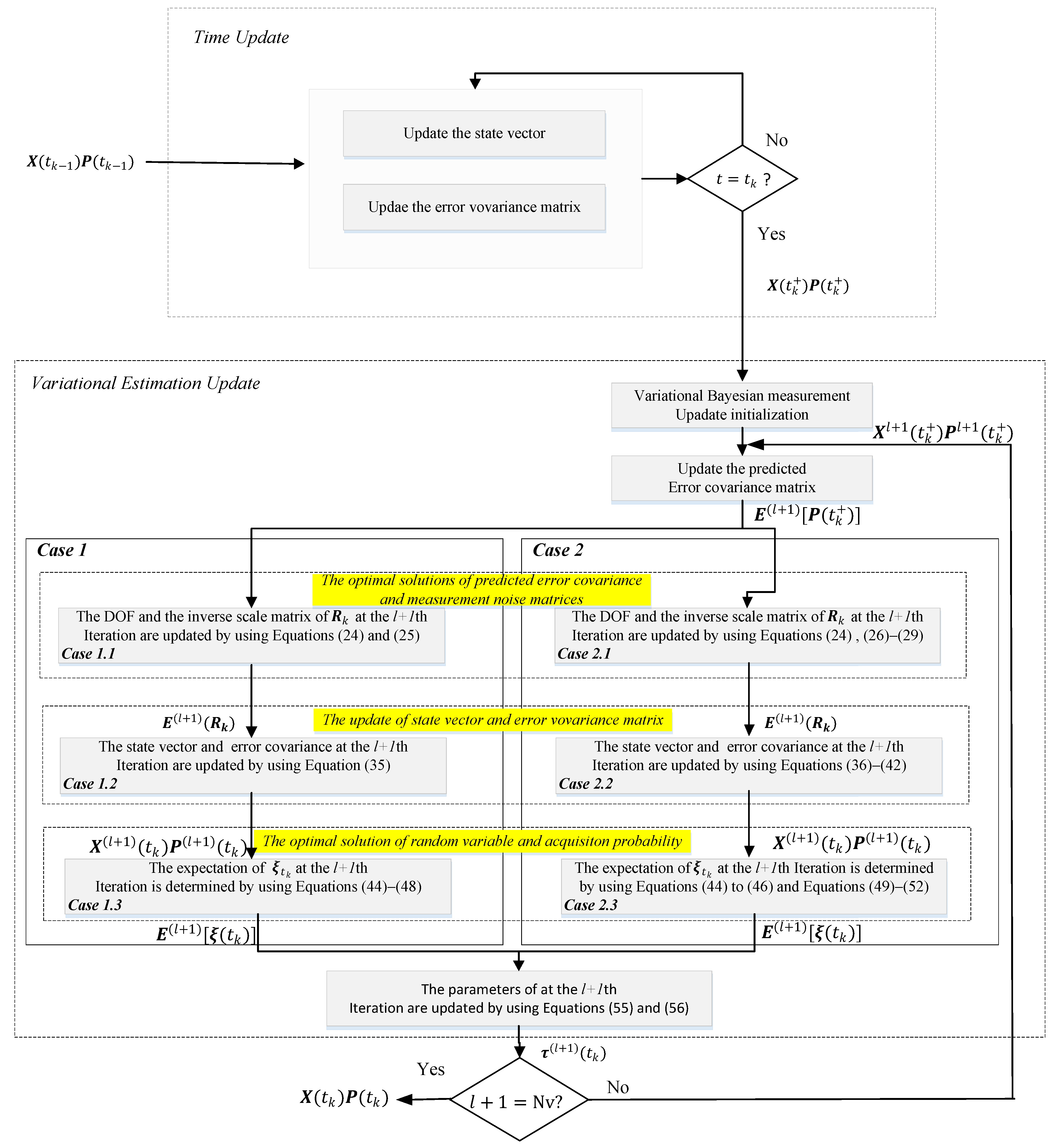
3.2. Proposed Optimal Variational Estimation in Navigation Information Acquisition

$\mathrm{Pro}\left[\mathsf{\Theta }|Z_{1:k}\right]$ is used to estimate the optimal solution of $\mathsf{\Theta }$. However, the joint posteriori PDF cannot be solved, so the variational Bayesian algorithm is introduced to search for an optimal PDF $\mathrm{q}(•)$ to characterize the joint posteriori PDF as:

$$\mathrm{Pro}\left[\mathsf{\Theta }|Z_{1:k}\right]\approx \mathrm{q}\left[X\left(t_k\right)\right]\mathrm{q}\left[P\left(t_k^{+}\right)\right]\mathrm{q}\left[R_k\right]\mathrm{q}\left[\xi \left(t_k\right)\right]\mathrm{q}\left[\tau \left(t_k\right)\right]$$

(18)

The optimal solutions satisfied the Equation (19).

$$\log \mathrm{q}\left(\kappa \right)={\mathrm{E}}_{{\mathsf{\Theta }}^{-\kappa }}\left\{\log \left[\mathrm{Pro}\left(\mathsf{\Theta },Z_{1:k}\right)\right]\right\}+C_{\kappa }$$

(19)

where $\mathrm{E}[•]$ is the expectation operation; ${\mathsf{\Theta }}^{-\kappa }$ refers to all the elements in $\mathsf{\Theta }$ except for $\kappa$; $C_{\kappa }$ is a constant related to $\kappa$.

The logarithm of $\mathrm{Pro}\left[\mathsf{\Theta },Z_{1:k}\right]$ is calculated as below:

$$\begin{array}{cc}\hfill \log \left[\mathrm{Pro}\left(\mathsf{\Theta },Z_{1:k}\right)\right]=& -\frac{1}{2}\xi \left(t_k\right)\left\{Z\left(t_k\right)-h\left[X\left(t_k\right)\right]\right\}-\frac{1}{2}\left[1-\xi \left(t_k\right)\right]Z^T\left(t_k\right)R_k^{-1}Z\left(t_k\right)\hfill \\ & -\frac{1}{2}\left[n_Z+u\left(t_k^{+}\right)+2\right]\log \left|R_k\right|-\frac{1}{2}{\left[X\left(t_k\right)-X\left(t_k^{+}\right)\right]}^T{P}^{-1}\left(t_k^{+}\right)\left[X\left(t_k\right)-X\left(t_k^{+}\right)\right]\hfill \\ & -\frac{1}{2}tr\left[U\left(t_k^{+}\right)R_k^{-1}\right]-\frac{1}{2}\left[n_x+t\left(t_k^{+}\right)+2\right]\log \left|P\left(t_k^{+}\right)\right|\hfill \\ & -\frac{1}{2}tr\left[T\left(t_k^{+}\right)P^{-1}\left(t_k^{+}\right)\right]+\xi \left(t_k\right)\log \left[\tau \left(t_k\right)\right]\hfill \\ & +\left[1-\xi \left(t_k\right)\right]\log \left[1-\tau \left(t_k\right)\right]+\left[\alpha \left(t_k^{+}\right)-1\right]\log \left[\tau \left(t_k\right)\right]\hfill \\ & +\left[\beta \left(t_k^{+}\right)-1\right]\log \left[1-\tau \left(t_k\right)\right]+C_{\epsilon }\hfill \end{array}$$

(20)

where $n_x$ indicates the dimension of $X\left(t_k\right)$; $n_Z$ indicates the dimension of $Z\left(t_k\right)$.

(1)

The optimal solutions of predicted error covariance and observation noise matrices.

Suppose $\kappa =P\left(t_k^{+}\right)$; then, the logarithm of $\mathrm{q}\left(\kappa \right)$ in iteration $l+1$ is written as:

$$\log q^{\left(l+1\right)}\left(\kappa \right)=-\frac{1}{2}\left[n_x+t^{\left(l\right)}\left(t_k^{+}\right)+2\right]\log \left|P^{\left(l\right)}\left(t_k^{+}\right)\right|-\frac{1}{2}tr\left\{\left[A_k^{\left(l\right)}+{{\rm T}}^{\left(l\right)}\left(t_k^{+}\right)\right]P^{-\left(l\right)}\left(t_k^{+}\right)\right\}+C_P$$

(21)

where $A_k^{\left(l\right)}=P^{\left(l\right)}\left(t_k\right)+\left[X^{\left(l\right)}\left(t_k\right)-X\left(t_k^{+}\right)\right]{\left[X^{\left(l\right)}\left(t_k\right)-X\left(t_k^{+}\right)\right]}^T$.

The DOF and inverse scale matrix of $P\left(t_k^{+}\right)$ in iteration $l+1$ are updated as:

$$\{\begin{array}{l}{t}^{\left(l+1\right)}\left(t_k\right)=t^{\left(l\right)}\left(t_k^{+}\right)+1\\ {{\rm T}}^{\left(l+1\right)}\left(t_k\right)=A_k^{\left(l\right)}+{{\rm T}}^{\left(l\right)}\left(t_k^{+}\right)\end{array}$$

(22)

Set $\kappa =R_k$; then, the logarithm of $\mathrm{q}\left(\kappa \right)$ is calculated in iteration l + 1 as:

$$\begin{array}{ll}\hfill \log {\mathrm{q}}^{\left(l+1\right)}\left(\kappa \right)=& -\frac{1}{2}\left[n_Z+u^{\left(l\right)}\left(t_k^{+}\right)+2\right]\log \left|R_k^{\left(l\right)}\right|\hfill \\ & -\frac{1}{2}tr\left\{\left[B_k^{\left(l\right)}+U_k^{\left(l\right)}\left(t_k^{+}\right)\right]R_k^{-\left(l\right)}\right\}+C_R\hfill \end{array}$$

(23)

where

$$\begin{array}{ll}{B}_k^{\left(l\right)}=& {\mathrm{E}}^{\left(l\right)}\left[\xi \left(t_k\right)\right]{\mathrm{E}}^{\left(l\right)}\left\{\left\{Z\left(t_k\right)-h\left[X\left(t_k\right)\right]\right\}{\left\{Z\left(t_k\right)-h\left[X\left(t_k\right)\right]\right\}}^T\right\}\hfill \\ & +\left\{1-{\mathrm{E}}^{\left(l\right)}\left[\xi \left(t_k\right)\right]\right\}{\mathrm{E}}^{\left(l\right)}\left[Z\left(t_k\right)Z^T\left(t_k\right)\right]\hfill \end{array}$$

(24)

Case 1.1: In iteration l, the expectation of $\left\{\left\{Z\left(t_k\right)-h\left[X\left(t_k\right)\right]\right\}{\left\{Z\left(t_k\right)-h\left[X\left(t_k\right)\right]\right\}}^T\right\}$ is calculated as:

$$\begin{array}{c}{\mathrm{E}}^{\left(l\right)}\left\{\left\{Z\left(t_k\right)-h\left[X\left(t_k\right)\right]\right\}{\left\{Z\left(t_k\right)-h\left[X\left(t_k\right)\right]\right\}}^T\right\}\\ ={\mathrm{E}}^{\left(l\right)}\left\{Z\left(t_k\right)-h\left[X^{\left(l\right)}\left(t_k\right)\right]+h\left[X^{\left(l\right)}\left(t_k\right)\right]-h\left[X\left(t_k\right)\right]\right\}\times {\left\{Z\left(t_k\right)-h\left[X^{\left(l\right)}\left(t_k\right)\right]+h\left[X^{\left(l\right)}\left(t_k\right)\right]-h\left[X\left(t_k\right)\right]\right\}}^T\\ =\left\{Z\left(t_k\right)-h\left[X^{\left(l\right)}\left(t_k\right)\right]\right\}{\left\{Z\left(t_k\right)-h\left[X^{\left(l\right)}\left(t_k\right)\right]\right\}}^T+H_k{P}^{\left(l\right)}\left(t_k^{+}\right)H_k^T\end{array}$$

(25)

Case 2.1: The expectation of $\left\{\left\{Z\left(t_k\right)-h\left[X\left(t_k\right)\right]\right\}{\left\{Z\left(t_k\right)-h\left[X\left(t_k\right)\right]\right\}}^T\right\}$ in iteration l is estimated by using the cubature rule.

The cubature points can be generated as:

$${\chi }_{i,k}^{\ast \left(l\right)}=X^{\left(l\right)}\left(t_k\right)+C_i^{\ast },i=1,2,\dots ,2n_x$$

(26)

where $C_i^{\ast }=\sqrt{n_x{P}^{\left(l\right)}\left(t_k\right)}{\left[I_x-I_x\right]}_i$; $I_x$ is the $n_x$-order identity matrix; ${[•]}_i$ represents column i of the matrix.

Then, the nonlinear integral, which is the expectation of $\left\{\left\{Z\left(t_k\right)-h\left[X\left(t_k\right)\right]\right\}{\left\{Z\left(t_k\right)-h\left[X\left(t_k\right)\right]\right\}}^T\right\}$ in iteration l, is calculated as:

$${\mathrm{E}}^{\left(l\right)}\left\{\left\{Z\left(t_k\right)-h\left[X\left(t_k\right)\right]\right\}{\left\{Z\left(t_k\right)-h\left[X\left(t_k\right)\right]\right\}}^T\right\}=\frac{1}{2n_x}{\displaystyle \sum _{i=1}^{2n_x}\left[Z_k^{\ast \left(l\right)}-h\left({\chi }_{i,k}^{\ast \left(l\right)}\right)\right]}{\left[Z_k^{\ast \left(l\right)}-h\left({\chi }_{i,k}^{\ast \left(l\right)}\right)\right]}^T$$

(27)

where $Z_k^{\ast \left(l\right)}$ is calculated by using Equation (28).

$$Z_k^{\ast \left(l\right)}=\frac{1}{2n_x}{\displaystyle \sum _{i=1}^{2n_x}h\left({\chi }_{i,k}^{\ast \left(l\right)}\right)}$$

(28)

When the measurement information is lost, ${\mathrm{E}}^{\left(l\right)}\left[Z\left(t_k\right)Z^T\left(t_k\right)\right]$ is derived as:

$${\mathrm{E}}^{\left(l\right)}\left[Z\left(t_k\right)Z^T\left(t_k\right)\right]=R_k^{\left(l\right)}$$

(29)

Remark 3.

In iteration l + 1, the update of DOF and the inverse scale matrix of $R_k$can be expressed as:

$$\{\begin{array}{l}{u}^{\left(l+1\right)}\left(t_k\right)=u^{\left(l\right)}\left(t_k^{+}\right)+1\\ U^{\left(l+1\right)}\left(t_k\right)=B_k^{\left(l\right)}+U^{\left(l\right)}\left(t_k^{+}\right)\end{array}$$

(30)

The inverse of $R_k$and inverse of $P\left(t_k^{+}\right)$can be determined by:

$$\{\begin{array}{l}{\mathrm{E}}^{\left(l+1\right)}\left(R_k^{-1}\right)={\mathrm{E}}^{\left(l\right)}\left[\xi \left(t_k\right)\right]\left[u^{\left(l+1\right)}\left(t_k\right)-n_Z-1\right]U^{-\left(l+1\right)}\left(t_k\right)\\ {\mathrm{E}}^{\left(l+1\right)}\left[P^{-1}\left(t_k^{+}\right)\right]=\left[t^{\left(l+1\right)}\left(t_k\right)-n_x-1\right]T^{-\left(l+1\right)}\left(t_k\right)\end{array}$$

(31)

The expectations of $R_k$and $P\left(t_k^{+}\right)$in iteration l + 1 are expressed as:

$$\{\begin{array}{l}{\mathrm{E}}^{\left(l+1\right)}\left(R_k\right)={\left[{\mathrm{E}}^{\left(l+1\right)}\left(R_k^{-1}\right)\right]}^{-1}\\ {\mathrm{E}}^{\left(l+1\right)}\left[P\left(t_k^{+}\right)\right]={\left\{{\mathrm{E}}^{\left(l+1\right)}\left[P^{-1}\left(t_k^{+}\right)\right]\right\}}^{-1}\end{array}$$

(32)

(2)

The update of state vector and error covariance matrix.

Set $\kappa =X\left(t_k\right)$; then, the logarithm of $\mathrm{q}\left(\kappa \right)$ is calculated in Equation (33) in iteration l + 1.

$$\begin{array}{cc}\hfill \log q^{\left(l+1\right)}\left(\kappa \right)=& -\frac{1}{2}\left\{1-{\mathrm{E}}^{\left(l\right)}\left[\xi \left(t_k\right)\right]\right\}{Z}^T\left(t_k\right){\mathrm{E}}^{\left(l+1\right)}\left(R_k^{-1}\right)Z\left(t_k\right)\hfill \\ & -\frac{1}{2}{\mathrm{E}}^{\left(l\right)}\left[\xi \left(t_k\right)\right]{\left\{Z\left(t_k\right)-h\left[X\left(t_k\right)\right]\right\}}^T\times {\mathrm{E}}^{\left(l+1\right)}\left(R_k^{-1}\right)\left\{Z\left(t_k\right)-h\left[X\left(t_k\right)\right]\right\}\hfill \\ & -\frac{1}{2}{\left[X\left(t_k\right)-X\left(t_k^{+}\right)\right]}^T{\mathrm{E}}^{\left(l+1\right)}\left[P^{-1}\left(t_k^{+}\right)\right]\left[X\left(t_k\right)-X\left(t_k^{+}\right)\right]+C_x\hfill \end{array}$$

(33)

In iteration l +1,the update of $q\left[X\left(t_k\right)\right]$ is:

$$q^{\left(l+1\right)}\left[X\left(t_k\right)\right]=N\left(X\left(t_k\right);X\left(t_k^{+}\right),P\left(t_k^{+}\right)\right)$$

(34)

Case 1.2: The measurement update is written based on the traditional Gaussian filter.

$$\{\begin{array}{l}{K}_k^{\left(l+1\right)}=P^{\left(l+1\right)}\left(t_k^{+}\right)H_k^T{\left[H_k{P}^{\left(l+1\right)}\left(t_k^{+}\right)H_k^T+R_k^{\left(l+1\right)}\right]}^{-1}\\ X^{\left(l+1\right)}\left(t_k\right)=X\left(t_k^{+}\right)+K_k^{\left(l+1\right)}{\mathrm{E}}^{\left(l\right)}\left[\xi \left(t_k\right)\right]\left[Z\left(t_k\right)-H_k{X}^{\left(l\right)}\left(t_k\right)\right]\\ P^{\left(l+1\right)}\left(t_k\right)=P^{\left(l+1\right)}\left(t_k^{+}\right)-K_k^{\left(l+1\right)}{H}_k{P}^{\left(l+1\right)}\left(t_k^{+}\right)\end{array}$$

(35)

Case 2.2: The measurement update is rewritten below.

The cubature points are selected by using Equation (36).

$${\chi }_{i,k}^{\ast \ast \left(l\right)}=X^{\left(l\right)}\left(t_k\right)+C_i^{\ast \ast },i=1,2,\dots ,2n_x$$

(36)

where $C_i^{\ast \ast }=\sqrt{n_x{P}^{\left(l+1\right)}\left(t_k^{+}\right)}{\left[\begin{array}{cc}{I}_x& -I_x\end{array}\right]}_i$.

The predicted measurement vector is calculated below:

$$Z_k^{\ast \ast \left(l\right)}=\frac{1}{2n_x}{\displaystyle \sum _{i=1}^{2n_x}h\left({\chi }_{i,k}^{\ast \ast \left(l\right)}\right)}$$

(37)

The cross covariance matrix $P_{xz}^{\left(l+1\right)}$ and measurement error covariance matrix $P_{zz}^{\left(l+1\right)}$ are calculated by Equations (38) and (39).

$$P_{xz}^{\left(l+1\right)}=\frac{{\mathrm{E}}^{\left(l\right)}\left[\xi \left(t_k\right)\right]}{2n_x}{\displaystyle \sum _{i=1}^{2n_x}\left[X^{\left(l\right)}\left(t_k\right)-{\chi }_{i,k}^{\ast \ast \left(l\right)}\right]}\left[Z_k^{\ast \ast \left(l\right)}-h\left({\chi }_{i,k}^{\ast \ast \left(l\right)}\right)\right]+\frac{\left(1-{\mathrm{E}}^{\left(l\right)}\right)\left[\xi \left(t_k\right)\right]}{2n_x}{\displaystyle \sum _{i=1}^{2n_x}\left[X^{\left(l\right)}\left(t_k\right)-{\chi }_{i,k}^{\ast \ast \left(l\right)}\right]}{\left(Z_k^{\ast \ast \left(l\right)}\right)}^T$$

(38)

$$P_{zz}^{\left(l+1\right)}=\frac{{\mathrm{E}}^{\left(l\right)}\left[\xi \left[t_k\right]\right]}{2n_x}{\displaystyle \sum _{i=1}^{2n_x}\left[Z_k^{\ast \ast \left(l\right)}-h\left({\chi }_{i,k}^{\ast \ast \left(l\right)}\right)\right]}{\left[Z_k^{\ast \ast \left(l\right)}-h\left({\chi }_{i,k}^{\ast \ast \left(l\right)}\right)\right]}^T+\left\{1-{\mathrm{E}}^{\left(l\right)}\left[\xi \left(t_k\right)\right]\right\}{Z}_k^{\ast \ast \left(l\right)}{\left(Z_k^{\ast \ast \left(l\right)}\right)}^T$$

(39)

Remark 4.

The derivation of Kalman gain $K_k^{\left(l+1\right)}$can be expressed as:

$$K_k^{\left(l+1\right)}=P_{xz}^{\left(l+1\right)}{P}_{zz}^{-\left(l+1\right)}$$

(40)

In iteration l + 1, $X\left(t_k\right)$and $P\left(t_k\right)$can be calculated as:

$$X^{\left(l+1\right)}\left(t_k\right)=X\left(t_k^{+}\right)+K_k^{\left(l+1\right)}\left[{\rm Z}\left(t_k\right)-Z_k^{\ast \ast \left(l\right)}\right]$$

(41)

$$P^{\left(l+1\right)}\left(t_k\right)=P^{\left(l+1\right)}\left(t_k^{+}\right)-K_k^{\left(l+1\right)}{P}_{zz}^{\left(l+1\right)}{\left(K_k^{\left(l+1\right)}\right)}^T$$

(42)

(3)

The optimal solutions of the random variable and acquisition probability.

Set $\kappa =\xi \left(t_k\right)$; the logarithm of $q\left(\kappa \right)$ in iteration l +1 is expressed as:

$$\begin{array}{cc}\hfill \log q^{\left(l+1\right)}\left(\kappa \right)=& -\frac{1}{2}\{{\xi }^{\left(l\right)}\left(t_k\right){\left\{Z\left(t_k\right)-h\left[X^{\left(l+1\right)}\left(t_k\right)\right]\right\}}^T\times {\mathrm{E}}^{\left(l+1\right)}\left(R_k^{-1}\right)\left\{Z\left(t_k\right)-h\left[X^{\left(l+1\right)}\left(t_k\right)\right]\right\}\}\hfill \\ & -\frac{1}{2}\left[1-{\xi }^{\left(l\right)}\left(t_k\right)\right]Z^T\left(t_k\right){\mathrm{E}}^{\left(l+1\right)}\left(R_k^{-1}\right)Z\left(t_k\right)+\left[1-{\xi }^{\left(l\right)}\left(t_k\right)\right]\log \left[1-{\tau }^{\left(l\right)}\left(t_k\right)\right]\hfill \\ & +{\xi }^{\left(l\right)}\left(t_k\right)\log \left[{\tau }^{\left(l\right)}\left(t_k\right)\right]+C_{\xi }\hfill \end{array}$$

(43)

The expectation of $\xi \left(t_k\right)$ in iteration l +1 is determined as:

$${\mathrm{E}}^{\left(l+1\right)}\left[\xi \left(t_k\right)\right]=\frac{a}{a+b}$$

(44)

where a and b are calculated in Equations (45) and (46), respectively.

$$a=\exp \left\{{\mathrm{E}}^{\left(l+1\right)}\left[\log \left({\tau }^{\left(l\right)}\left(t_k\right)\right)\right]-\frac{1}{2}tr\left[D_k^{\left(l+1\right)}{\mathrm{E}}^{\left(l+1\right)}\left(R_k^{-1}\right)\right]\right\}$$

(45)

$$b=\exp \left\{{\mathrm{E}}^{\left(l+1\right)}\left[\log \left(1-{\tau }^{\left(l\right)}\left(t_k\right)\right)\right]-\frac{1}{2}tr\left[E_k^{\left(l+1\right)}{\mathrm{E}}^{\left(l+1\right)}\left(R_k^{-1}\right)\right]\right\}$$

(46)

where $D_k^{\left(l+1\right)}$ and $E_k^{\left(l+1\right)}$ are estimated by Equations (47)–(52).

Case 1.3: $D_k^{\left(l+1\right)}$ and $E_k^{\left(l+1\right)}$ are written as:

$$\begin{array}{ll}\hfill D_k^{\left(l+1\right)}& ={\mathrm{E}}^{\left(l+1\right)}\left\{\left\{Z\left(t_K\right)-h\left[X\left(t_K\right)\right]\right\}{\left\{Z\left(t_K\right)-h\left[X\left(t_K\right)\right]\right\}}^T\right\}\hfill \\ & =\left\{\left\{Z\left(t_K\right)-h\left[X^{\left(l+1\right)}\left(t_K\right)\right]\right\}{\left\{Z\left(t_K\right)-h\left[X^{\left(l+1\right)}\left(t_K\right)\right]\right\}}^T\right\}+H_k{P}^{\left(l+1\right)}\left(t_k^{+}\right)H_k^T\hfill \end{array}$$

(47)

$$E_k^{\left(l+1\right)}={\mathrm{E}}^{\left(l+1\right)}\left(Z_k{Z}_k^T\right)$$

(48)

Case 2.3: $D_k^{\left(l+1\right)}$ and $E_k^{\left(l+1\right)}$ are written as follows.

The cubature points are selected by using Equation (49).

$${\chi }_{i,k}^{\ast \ast \ast \left(l+1\right)}=X^{\left(l+1\right)}\left(t_k\right)+C_i^{\ast \ast \ast }i=1,2,\dots ,2n_x$$

(49)

where $C_i^{\ast \ast \ast }=\sqrt{n_x{P}^{\left(l+1\right)}\left(t_k\right)}{\left[\begin{array}{cc}{I}_x& -I_x\end{array}\right]}_i$.

$$D_k^{\left(l+1\right)}=\frac{1}{2n_x}{\displaystyle \sum _{i=1}^{2n_x}\left[Z_k^{\ast \ast \ast \left(l+1\right)}-h\left({\chi }_{i,k}^{\ast \ast \ast \left(l+1\right)}\right)\right]}{\left[Z_k^{\ast \ast \ast \left(l+1\right)}-h\left({\chi }_{i,k}^{\ast \ast \ast \left(l+1\right)}\right)\right]}^T$$

(50)

$$E_k^{\left(l+1\right)}=\frac{1}{2n_x}{\displaystyle \sum _{i=1}^{2n_x}h\left({\chi }_{i,k}^{\ast \ast \ast \left(l+1\right)}\right)}{h}^T\left({\chi }_{i,k}^{\ast \ast \ast \left(l+1\right)}\right)$$

(51)

Then, $Z_k^{\ast \ast \ast \left(l+1\right)}$ is calculated as Equation (52).

$$Z_k^{\ast \ast \ast \left(l+1\right)}=\frac{1}{2n_x}{\displaystyle \sum _{i=1}^{2n_x}h\left({\chi }_{i,k}^{\ast \ast \ast \left(l+1\right)}\right)}$$

(52)

Remark 5.

The expectations of $\tau \left(t_k\right)$and $\left[1-\tau \left(t_k\right)\right]$in iteration l + 1 are calculated by using Equation (53).

$$\{\begin{array}{l}{\mathrm{E}}^{\left(l+1\right)}\left\{\log \left[ \tau \left(t_k\right)\right]\right\}=\psi \left[{\alpha }^{\left(l\right)}\left(t_k\right)\right]-\psi \left[{\alpha }^{\left(l\right)}\left(t_k\right)+{\beta }^{\left(l\right)}\left(t_k\right)\right]\\ {\mathrm{E}}^{\left(l+1\right)}\left\{\log \left[ 1-\tau \left(t_k\right)\right]\right\}=\psi \left[{\beta }^{\left(l\right)}\left(t_k\right)\right]-\psi \left[{\alpha }^{\left(l\right)}\left(t_k\right)+{\beta }^{\left(l\right)}\left(t_k\right)\right]\end{array}$$

(53)

where $\psi (•)$is the digamma function.

Set $\kappa =\tau \left(t_k\right)$; the update of $q\left(\kappa \right)$ in iteration l + 1 can be expressed as:

$$q^{\left(l+1\right)}\left(\kappa \right)=B\left(\kappa ;{\alpha }^{\left(l+1\right)}\left(t_k\right),{\beta }^{\left(l+1\right)}\left(t_k\right)\right)$$

(54)

The parameters of $\tau \left(t_k\right)$ in iteration l + 1 are calculated by using Equation (55).

$$\{\begin{array}{l}{\alpha }^{\left(l+1\right)}\left(t_k\right)={\alpha }^{\left(l+1\right)}\left(t_k^{+}\right)-{\mathrm{E}}^{\left(l+1\right)}\left[\xi \left(t_k\right)\right]+1\\ {\beta }^{\left(l+1\right)}\left(t_k\right)={\beta }^{\left(l+1\right)}\left(t_k^{+}\right)+{\mathrm{E}}^{\left(l+1\right)}\left[\xi \left(t_k\right)\right]\end{array}$$

(55)

The updates of ${\alpha }^{\left(l+1\right)}\left(t_k^{+}\right)$ and ${\beta }^{\left(l+1\right)}\left(t_k^{+}\right)$ are derived by:

$$\{\begin{array}{l}{\alpha }^{\left(l+1\right)}\left(t_k^{+}\right)=\rho {\alpha }^{\left(l\right)}\left(t_k\right)\\ {\beta }^{\left(l+1\right)}\left(t_k^{+}\right)=\rho {\beta }^{\left(l\right)}\left(t_k\right)\end{array}$$

(56)

After Nv iterations, the variational Bayesian approximation of the PDF is given as:

$$q\left[P\left(t_k^{+}\right)\right]\approx q^{\left(\mathrm{Nv}\right)}\left[P\left(t_k^{+}\right)\right]=\mathrm{IW}\left(P\left(t_k^{+}\right);t^{\left(\mathrm{Nv}\right)}\left(t_k\right),T^{\left(\mathrm{Nv}\right)}\left(t_k\right)\right)$$

(57)

$$q\left(R_k\right)\approx q^{\left(\mathrm{Nv}\right)}\left(R_k\right)=\mathrm{IW}\left(R_k;u^{\left(\mathrm{Nv}\right)}\left(t_k\right),U^{\left(\mathrm{Nv}\right)}\left(t_k\right)\right)$$

(58)

$$q\left[X\left(t_k\right)\right]\approx q^{\left(\mathrm{Nv}\right)}\left[X\left(t_k\right)\right]=N\left(X\left(t_k\right);X^{\left(\mathrm{Nv}\right)}\left(t_{{}_k}^{+}\right),P^{\left(\mathrm{Nv}\right)}\left(t_{{}_k}^{+}\right)\right)$$

(59)

$$\xi \left(t_k\right)\approx {\xi }^{\left(\mathrm{Nv}\right)}\left(t_k\right)={\mathrm{E}}^{\left(\mathrm{Nv}\right)}\left[\xi \left(t_k\right)\right]$$

(60)

$$q\left[\tau \left(t_k\right)\right]\approx q^{\left(\mathrm{Nv}\right)}\left[\tau \left(t_k\right)\right]=B\left(\tau \left(t_k\right);{\alpha }^{\left(\mathrm{Nv}\right)}\left(t_k\right),{\beta }^{\left(\mathrm{Nv}\right)}\left(t_k\right)\right)$$

(61)

The flowchart of the SVEF is shown in Figure 2. The derivatives of $X\left(t_{k-1}\right)$ and $P\left(t_{k-1}\right)$ are calculated as Equations (15) and (16), respectively. When the time is equal to k, $X\left(t_k^{+}\right)$ and $P\left(t_k^{+}\right)$ are derived by using Equation (17). At the start of the variation estimation update, the number of iterations l is set to 0. Then, $X^{\left(l\right)}\left(t_k^{+}\right)=X\left(t_k^{+}\right)$ and $P^{\left(l\right)}\left(t_k^{+}\right)=P\left(t_k^{+}\right)$ are initialized for the subsequent variational estimation update. In iteration l + 1 step at time k, firstly, the calculations of $P\left(t_k^{+}\right)$ and $R_k$ are performed by using their DOFs and inverse scale matrices, respectively. Then, $X\left(t_k\right)$ and $P\left(t_k\right)$ in iteration l + 1 are estimated in linear or nonlinear forms by using Equations (35)–(42). Finally, the information about $\xi \left(t_k\right)$ and $\tau \left(t_k\right)$ is updated by using Equations (44)–(56). After iteration Nv, $X\left(t_k\right)$ and $P\left(t_k\right)$ are accurately determined at time k. The pseudocode is represented in Algorithm 1.

Algorithm 1: The proposed switched variational estimation filtering algorithm.

Input:$X\left(t_{k-1}\right)$, $P\left(t_{k-1}\right)$, $\xi \left(t_{k-1}\right)$, $\tau \left(t_{k-1}\right)$. Time Update: for i = 0:0.01:1 Update $X(t_k^{+})$ and $P(t_k^{+})$ using Equations (15)–(17); end Variational Estimation Update: Variational estimation initialization: $X^{(l)}(t_k)$, $P^{(l)}(t_k)$. for l = 0: Nv − 1 (1) The optimal solutions of the predicted error covariance and measurement noise matrices. The DOF and inverse scale matrix of $P(t_k^{+})$ in iteration l + 1 are updated by using Equation (22). The update of the DOF and the inverse scale matrix of $R_k$ in iteration l + 1: Case 1.1 updated by using Equations (24) and (25). Case 2.1 updated by using Equations (24), (26)–(29). $P(t_k^{+})$ and $R_k$ are calculated by Equations (30)–(32). (2) The update of state vector and error covariance matrix in iteration l + 1. Case 1.2 updated by using Equation (35). Case 2.2 updated by using Equations (36)–(42). (3) The optimal solutions of the random variable and acquisition probability. The expectation of $\xi \left(t_k\right)$ in iteration l + 1: Case 1.3 determined by using Equations (44)–(48). Case 2.3 determined by using Equations (44)–(46) and (49)–(52). The parameters of $\tau \left(t_k\right)$ in iteration l + 1 are updated by using Equations (55)–(56) End Output: $X(t_k)$ and $P(t_k)$.

4. Experiments and Results

Complex and changeable underwater environments bring huge errors and nonlinearity to MEMS-based inertial sensors mounted on AUVs. Moreover, the magnetometers used to compensate for the inertial sensor error are disturbed by the variable marine environment. Therefore, establishing a model that can accurately describe the measurement noise is difficult, resulting in the measurement noise assumption of the navigation determination algorithm being not in accord with the real noise information, which greatly reduces the state estimation precision. For the accuracy and robustness validation of the proposed SVEF method, realistic underwater tests were carried out. The underwater navigation system was based on MEMS technology and was mainly made up of inertial sensors aided by magnetic sensors. The position and speed solutions were provided by the above sensors mounted on the AUV as it worked in the water. Once the underwater vehicle surfaced, GPS was used to update the navigation information. The camera was used for under water image acquisition. Moreover, to establish a reliable experimental platform, the underwater vehicle was also equipped with some navigation devices. The performance comparison between the proposed SVEF and the conventional filtering algorithms was carried out through a series of underwater experiments. The time interval was 0.01 s for the process model, and the time interval was 1 s for the observation model.

Remark 6.

The normalized process noise covariance matrix and measurement noise covariance matrix are defined as $\overline{Q}\left(t\right)$and$\overline{R}\left(t_k\right)$, respectively. Limited by experimental conditions, the real experiment was performed in a lake. However, to simulate complicated and variable marine environments, the complex process noise and the measurement noise were defined as:

$$Q\left(t\right)=\{\begin{array}{ll}\overline{Q}\left(t\right)\hfill & {\mathrm{P}}_S\left(0\le k_1<0.3\right)\hfill \\ 10\overline{Q}\left(t\right)\hfill & {\mathrm{P}}_m\left(0.3\le k_1<0.7\right)\hfill \\ 20\overline{Q}\left(t\right)\hfill & {\mathrm{P}}_l\left(0.7\le k_1\le 1\right)\hfill \end{array}$$

(62)

$$R\left(t\right)=\{\begin{array}{ll}\overline{R}\left(t\right)\hfill & {\mathrm{P}}_S\left(0\le k_2<0.4\right)\hfill \\ 10\overline{R}\left(t\right)\hfill & {\mathrm{P}}_m\left(0.4\le k_2<0.6\right)\hfill \\ 20\overline{R}\left(t\right)\hfill & {\mathrm{P}}_l\left(0.6\le k_2\le 1\right)\hfill \end{array}$$

(63)

where k₁ and k₂ represent preset uncorrelated random numbers. The probability interval [0, 1] is roughly divided into three segments, namely [0, 0.3], [0.3, 0.7], and [0.7, 1], which indicate low, moderate, and high impacts on noise, respectively. ${\mathrm{P}}_S(•)$, ${\mathrm{P}}_m(•)$, and ${\mathrm{P}}_l(•)$refer to the different probabilities under low, moderate, and high noises, respectively. The definition of the observation noise matrix is similar. The probability interval [0, 1] is roughly divided into three segments, namely [0, 0.4], [0.4, 0.6], and [0.6, 1], which indicate low, moderate, and high impacts on the noise, respectively.

The root mean square error (RMSE) of the position was applied to evaluate the performance of these algorithms. The definition of RMSE is:

$$\mathrm{RMSE}=\frac{1}{\mathrm{M}}{\displaystyle \sum _{k=1}^{\mathrm{M}}\sqrt{{\left[x\left(t_k\right)-x_k^r\right]}^2+{\left[y\left(t_k\right)-y_k^r\right]}^2}}$$

(64)

where $x\left(t_k\right)$ and $y\left(t_k\right)$ are the estimated east and north positions, respectively; $x_k^r$ and $y_k^r$ are the reference east and north positions, respectively; M is the number of the time sequence. The initial parameter settings are shown in

Table 1. Parameter settings.

Initialization Parameter	Value
$P\left(t_0\right)$	${10}^2\times diag[10{(\mathrm{m})}^2,1{(\mathrm{m}/\mathrm{s})}^2,10{(\mathrm{m})}^2,1{(\mathrm{m}/\mathrm{s})}^2,10{(\mathrm{m})}^2,1{(\mathrm{m}/\mathrm{s})}^2]$
$\overline{Q}\left(t_0\right)$	${10}^{-7}\times diag[100{(\mathrm{m})}^2,1{(\mathrm{m}/\mathrm{s})}^2,100{(\mathrm{m})}^2,1{(\mathrm{m}/\mathrm{s})}^2,100{(\mathrm{m})}^2,1{(\mathrm{m}/\mathrm{s})}^2]$
${\overline{R}}_k\left(\mathrm{nonlinear}\right)$	${10}^{-5}\times diag[1{(\mathrm{m})}^2,1{(\mathrm{m})}^2,1(\mathrm{deg})]$
${\overline{R}}_k\left(\mathrm{linear}\right)$	${10}^{-5}\times diag[1{(\mathrm{m})}^2,1{(\mathrm{m})}^2,1{(\mathrm{m})}^2]$

.

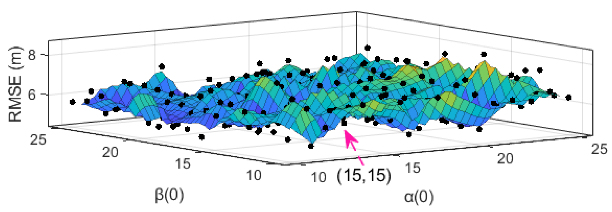
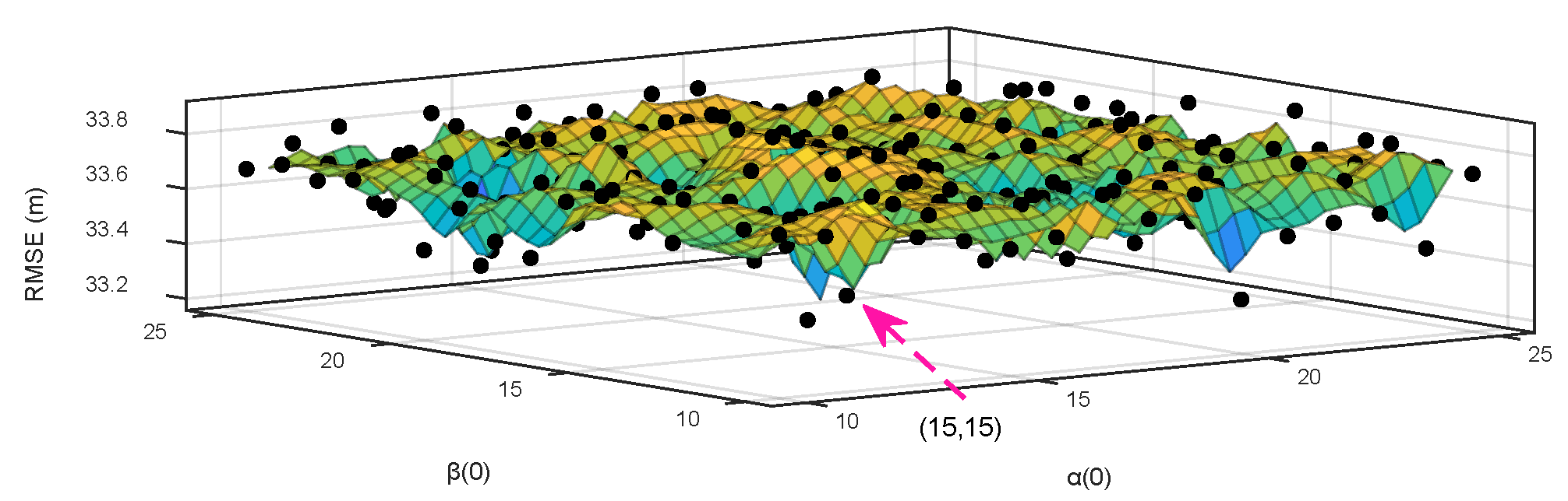
4.1. Selection of Initialization Values

Remark 7.

The initialization values of $\alpha \left(t_k\right)$and $\beta \left(t_k\right)$influence the estimation accuracy; experiments were employed to find the optimal solutions of $\alpha \left(0\right)$and $\beta \left(0\right)$. When $\alpha \in \left[1,10\right)$and $\beta \in \left[1,10\right)$, the algorithm was easily divergent, and when$\alpha \in \left(25,+\infty \right)$and $\beta \in \left(25,+\infty \right)$, the algorithm also diverged. Therefore, the range of the parameters was set as $\alpha \in \left[10,25\right]$and $\beta \in \left[10,25\right]$in the following experiments.

When the observation equation is linear, the solutions are as expressed in Figure 3. When the observation equation is nonlinear, the solutions are as denoted in Figure 4. From Figure 3 and Figure 4, it can be concluded that $\alpha \left(0\right)$ and $\beta \left(0\right)$ impact the RMSE. From the results of experiments, $\left(\alpha \left(0\right),\beta \left(0\right)\right)=\left(15,15\right)$ was chosen as an optimal solution to guarantee an algorithm with better accuracy and robustness.

Remark 8.

For the robustness verification of the proposed SVEF, we compared the proposed SVEF algorithm and other conventional algorithms by using the Monte Carlo (MC) method. The definition of MC RMSE is:

$$\mathrm{MC}\mathrm{RMSE}=\frac{1}{mc}{\displaystyle \sum _{j=1}^{mc}\mathrm{RMSE}\left(j\right)}$$

(65)

where $\mathrm{RMSE}\left(j\right)$refers to the RMSE at the jth Monte Carlo operation; mc denotes the total number of Monte Carlo operations, which was set to 100.

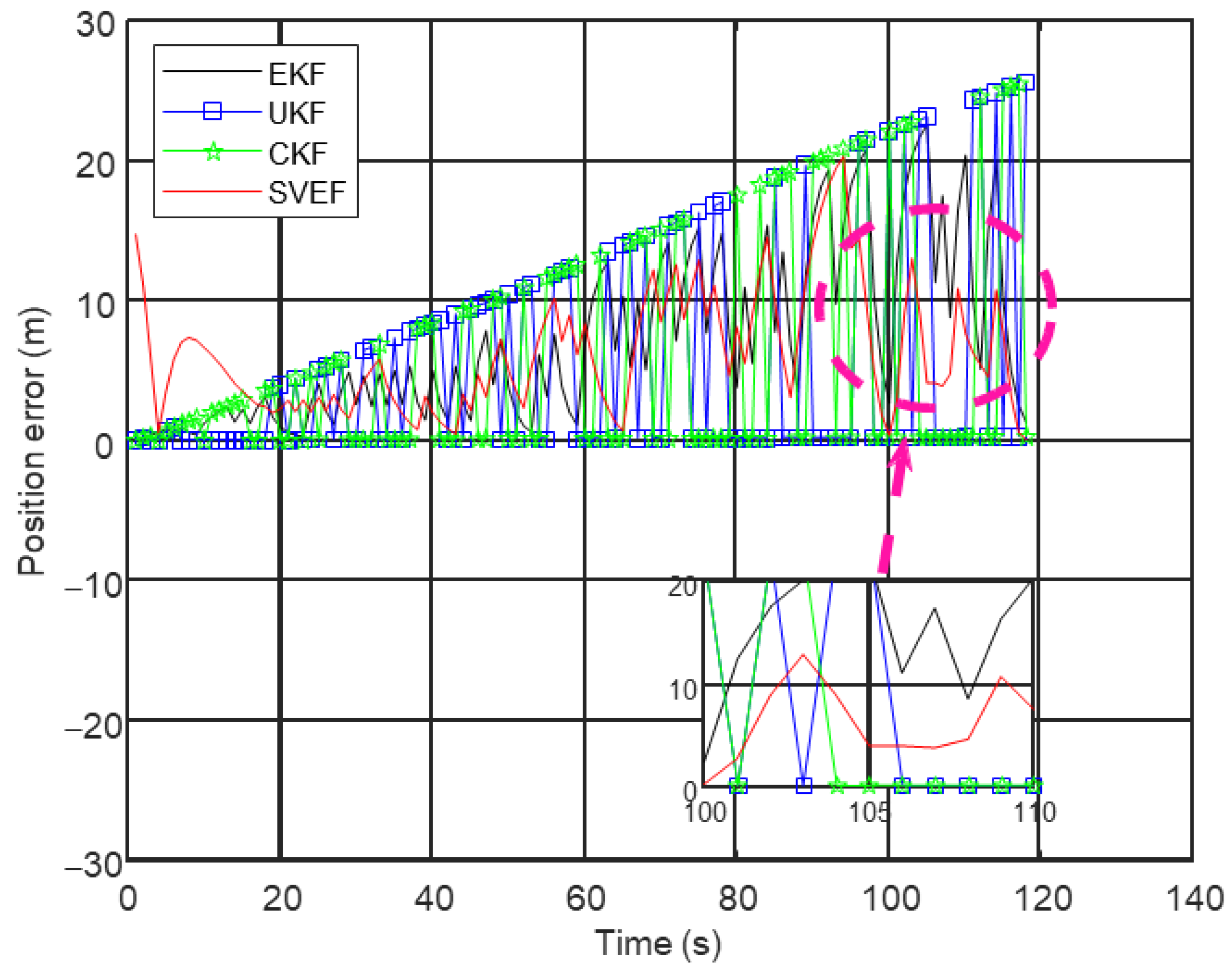
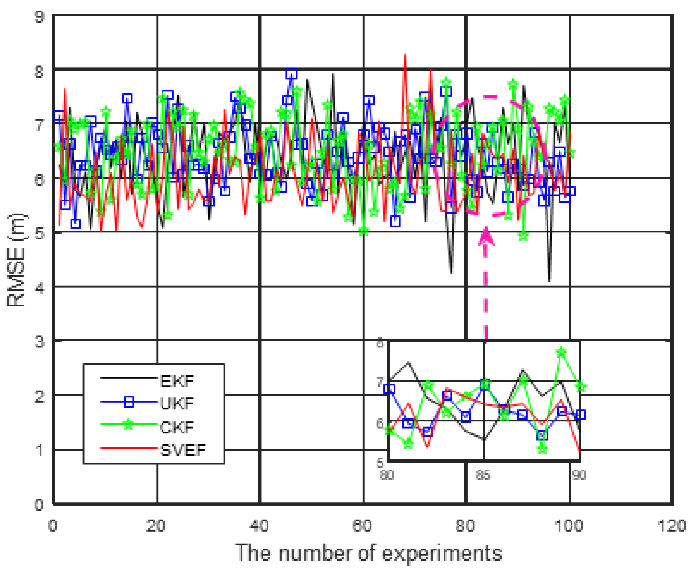
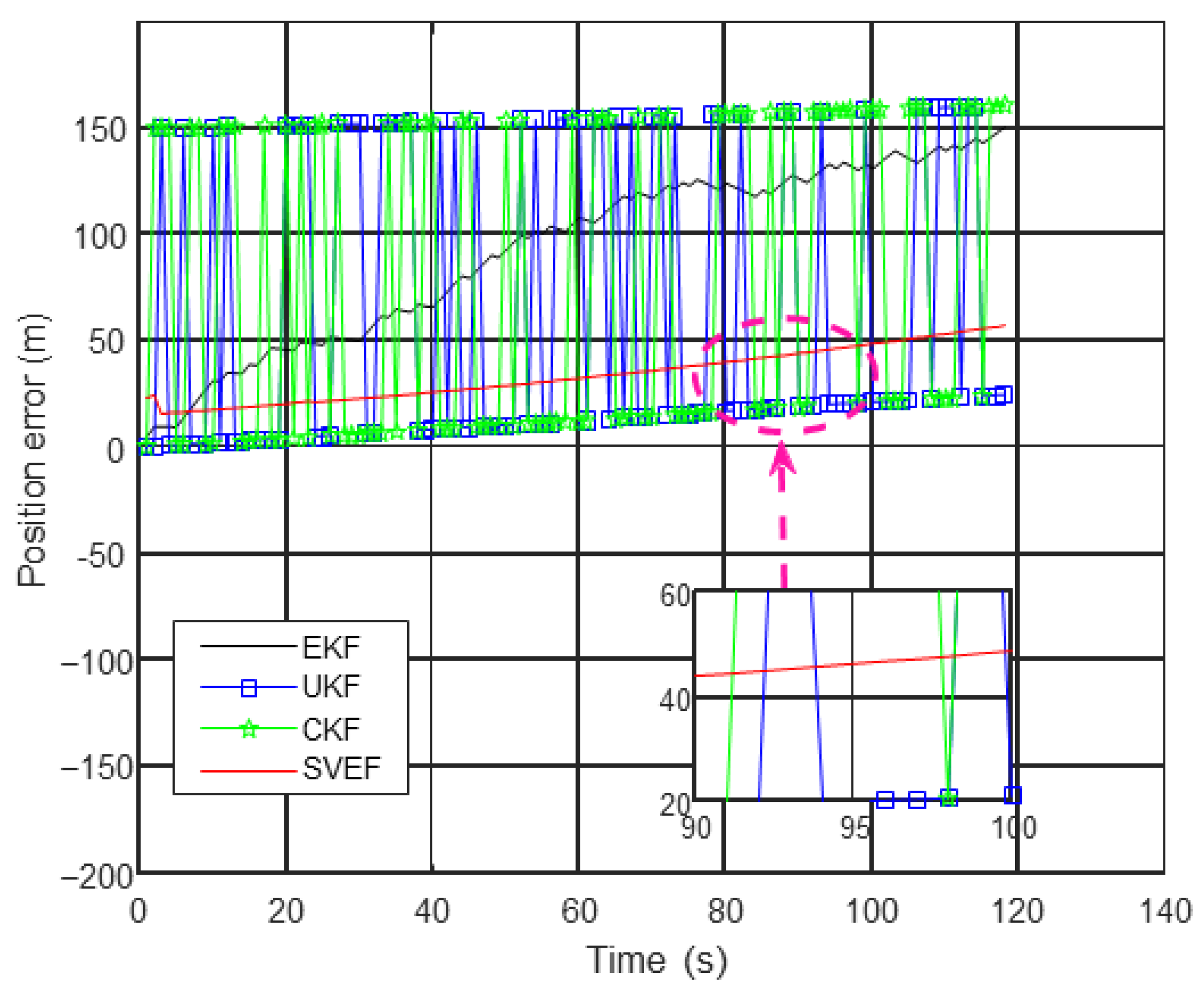
4.2. Comparison of State Estimation Algorithms

• Case 1: The measurement model is linear

In Case 1, the measurement vector was $Z\left(t_k\right)={\left[\begin{array}{ccc}x\left(t_k\right)& y\left(t_k\right)& z\left(t_k\right)\end{array}\right]}^T$. Figure 5 shows that the proposed SVEF achieved the best performance among all the comparison methods. Figure 6 shows that the robustness of SVEF was also the best among all compared algorithms. Aiming to more comprehensively evaluate the performance of these four methods,

Table 2. MC RMSE for different algorithms.

Algorithms	EKF	UKF	CKF	SVEF
MC RMSE (m)	6.6054	6.4225	6.5284	6.0907

also shows the calculated MC RMSE values. Table 2 shows that the MC RMSE value of SVEF was the smallest of the four algorithms. The improvement in the MC RMSE was about 7.79% over EKF, 5.17% over UKF, and 6.70% over CKF.

The traditional EKF uses the partial derivative to linearize the nonlinear process and measurement functions. However, truncation errors are introduced when calculating the Kalman gain, so that the errors of $X\left(t_k\right)$ and $P\left(t_k\right)$ become larger. The sample method for UKF and CKF is fundamentally the sample of a few points. When the dimensions of the state vector $n_x$ are more than three, the weight function of the UKF central sampling point is negative, but, in reality, the UKF and CKF have similar accuracies when the dimensions of state vector $n_x$ are less than seven. The proposed SVEF uses the VE method to update the state vector in real time in each iteration process, and a predicted error covariance matrix with high accuracy is achieved.

• Case 2: The measurement model is nonlinear

In Case 2, the measurement vector was selected as $Z\left(t_k\right)={\left[\begin{array}{ccc}r\left(t_k\right)& d\left(t_k\right)& \theta \left(t_k\right)\end{array}\right]}^T$. Figure 7 shows that the proposed SVEF achieved the best performance among the four algorithms. It is easy to see from Figure 7 MISSING that the robustness of SVEF was better than that of the other three algorithms. To more comprehensively evaluate the performance of these four methods, Figure 8 and

Table 3. MC RMSE for different algorithms.

Algorithms	EKF	UKF	CKF	SVEF
MC RMSE (m)	90.6664	84.0154	82.9580	33.6932

show the calculated MC RMSE values. The MC RMSE value of the SVEF was the smallest of the four algorithms. The improvement in the MC RMSE was about 62.84% over EKF, 59.90% over UKF, and 59.39% over CKF.

When the noises become complex and time-varying, there is a risk of losing measurement information. The above experimental results indicated that the SVEF performs better than the EKF, UKF, and CKF in dealing with the noise loss problem. Measurement information may be missing due to the interference of large noise with the sensor; therefore, precise noise information is difficult to obtain. In SVEF, $R_k$, $P\left(t_k^{+}\right)$, $\xi \left(t_k\right)$, and $\tau \left(t_k\right)$ can be adaptively adjusted to guarantee filtering stability. The problems of variable noise and measurement information loss lead to inaccuracy of the Kalman gain calculation and, thus, state variable divergence. The EKF cannot provide an accurate estimation of the state vector. The estimation effect of UKF relies on the weighting function. However, once the state dimension of the UKF is higher than three, the adjustment parameter becomes negative. In the presence of complex noise, the UKF cannot be able to obtain an accurate estimation. Therefore, the performance of UKF under complex noise conditions is also very poor. Although CKF overcomes the deficiencies of the EKF and UKF in some areas, CKF cannot obtain an accurate noise model, resulting in poor positioning performance. The loss of measurement information has a serious effect on $P_{xz}^{\left(l+1\right)}$ and $P_{zz}^{\left(l+1\right)}$, where the Kalman gain is also influenced. For the above problems, the proposed SVEF algorithm can achieve better results. We concluded that compared with other algorithms, the SVEF has a more accurate positioning effect for underwater vehicles.

5. Conclusions

The complex and variable ocean environment poses huge difficulties to the precise localization of MEMS-grade navigation systems mounted on AUVs. In addition, because the sampling frequency of the time update is 100 times higher than that of the measurement update, the ocean environment is not conducive to obtaining high-precision AUV positions. Obtaining accurate state estimates is difficult for conventional algorithms. The accuracy and robustness of the proposed SVEF were proved in theory and evaluated through a series of underwater experiments. The results demonstrated that SVEF achieves better AUV position estimation results than EKF, UKE, and CKF, even in the case of variations in measurement error and loss of measurement information. The SVEF can obtain more accurate estimations and error covariance matrices of states. Additionally, the state estimate is efficiently acquired by the SVEF and its robustness is excellent.

References

1. Teeneti, C.R.; Truscott, T.T.; Beal, D.N.; Pantic, Z. Review of Wireless Charging Systems for Autonomous Underwater Vehicles. IEEE J. Oceanic. Eng. 2021, 46, 68–87. [Google Scholar] [CrossRef]
2. Jiang, Y.; Feng, C.; He, B.; Guo, J.; Wang, D.; Lv, P.-F. Actuator fault diagnosis in autonomous underwater vehicle based on neural network. Sens. Actuator A Phys. 2021, 324, 112668. [Google Scholar] [CrossRef]
3. Huang, H.; Tang, J.; Liu, C.; Zhang, B.; Wang, B. Variational Bayesian-Based Filter for Inaccurate Input in Underwater Navigation. IEEE Trans. Veh. Technol. 2021, 70, 8441–8452. [Google Scholar] [CrossRef]
4. Xiong, Z.; Wu, M.; Cao, J.; Liu, Y.; Yu, R.; Cai, S. An Underwater Gravimetry Method Using Inertial Navigation System and Depth Gauge Based on Trajectory Constraint. IEEE Geosci. Remote Sens. Lett. 2021, 18, 1510–1514. [Google Scholar] [CrossRef]
5. Xiong, Z.; Cao, J.; Wu, M.; Cai, S.; Yu, R.; Wang, M. A Method for Underwater Dynamic Gravimetry Combining Inertial Navigation System, Doppler Velocity Log, and Depth Gauge. IEEE Geosci. Remote Sens. Lett. 2020, 17, 1294–1298. [Google Scholar] [CrossRef]
6. Donovan, G.T. Position Error Correction for an Autonomous Underwater Vehicle Inertial Navigation System (INS) Using a Particle Filter. IEEE J. Oceanic. Eng. 2012, 37, 431–445. [Google Scholar] [CrossRef]
7. Lu, J.; Xie, L. Ocean Vehicle Inertial Navigation Method based on Dynamic Constraints. J. Navig. 2018, 71, 1553–1566. [Google Scholar] [CrossRef]
8. Lv, P.-F.; He, B.; Guo, J. Position Correction Model Based on Gated Hybrid RNN for AUV Navigation. IEEE Trans. Veh. Technol. 2021, 70, 5648–5657. [Google Scholar] [CrossRef]
9. Mahboub, V.; Mohammadi, D. A Constrained Total Extended Kalman Filter for Integrated Navigation. J. Navig. 2018, 71, 971–988. [Google Scholar] [CrossRef]
10. Yao, Y.; Xu, X.; Yang, D.; Xu, X. An IMM-UKF Aided SINS/USBL Calibration Solution for Underwater Vehicles. IEEE Trans. Veh. Technol. 2020, 69, 3740–3747. [Google Scholar] [CrossRef]
11. Wang, G.; Xu, X.; Zhang, T. M-M Estimation-Based Robust Cubature Kalman Filter for INS/GPS Integrated Navigation System. IEEE Trans. Instrum. Meas. 2021, 70, 9501511. [Google Scholar] [CrossRef]
12. Karmozdi, A.; Hashemi, M.; Salarieh, H.; Alasty, A. INS-DVL Navigation Improvement Using Rotational Motion Dynamic Model of AUV. IEEE Sens. J. 2020, 20, 14329–14336. [Google Scholar] [CrossRef]
13. Kepper, J.H.; Claus, B.C.; Kinsey, J.C. A Navigation Solution Using a MEMS IMU, Model-Based Dead-Reckoning, and One-Way-Travel-Time Acoustic Range Measurements for Autonomous Underwater Vehicles. IEEE J. Oceanic. Eng. 2019, 44, 664–682. [Google Scholar] [CrossRef]
14. Song, S.; Liu, J.; Guo, J.; Wang, J.; Xie, Y.; Cui, J.-H. Neural-Network-Based AUV Navigation for Fast-Changing Environments. IEEE Internet Things J. 2020, 7, 9773–9783. [Google Scholar] [CrossRef]
15. Huang, Y.; Zhang, Y.; Xu, B.; Wu, Z.; Chambers, J.A. A New Adaptive Extended Kalman Filter for Cooperative Localization. IEEE Trans. Aerosp. Electron. Syst. 2018, 54, 353–368. [Google Scholar] [CrossRef]
16. Sabzevari, D.; Chatraei, A. INS/GPS Sensor Fusion based on Adaptive Fuzzy EKF with Sensitivity to Disturbances. IET Radar Sonar Navig. 2021, 15, 1535–1549. [Google Scholar] [CrossRef]
17. Noureldin, A.; Karamat, T.B.; Eberts, M.D.; El-Shafie, A. Performance Enhancement of MEMS-Based INS/GPS Integration for Low-Cost Navigation Applications. IEEE Trans. Veh. Technol. 2009, 58, 1077–1096. [Google Scholar] [CrossRef]
18. Duník, J.; Biswas, S.K.; Dempster, A.G.; Pany, T.; Closas, P. State Estimation Methods in Navigation: Overview and Application. IEEE Aerosp. Electron. Syst. Mag. 2020, 35, 16–31. [Google Scholar] [CrossRef]
19. Jiang, Z.; Zhou, W.; Li, H.; Mo, Y.; Ni, W.; Huang, Q. A New Kind of Accurate Calibration Method for Robotic Kinematic Parameters Based on the Extended Kalman and Particle Filter Algorithm. IEEE Trans. Ind. Electron. 2018, 65, 3337–3345. [Google Scholar] [CrossRef]
20. Lyu, X.; Hu, B.; Li, K.; Chang, L. An Adaptive and Robust UKF Approach Based on Gaussian Process Regression-Aided Variational Bayesian. IEEE Sens. J. 2021, 21, 9500–9514. [Google Scholar] [CrossRef]
21. Yang, Y.; Bin, L.; Xinjie, W.; Lijian, Y. Application of Adaptive Cubature Kalman Filter to In-Pipe Survey System for 3D Small-Diameter Pipeline Mapping. IEEE Sens. J. 2020, 20, 6331–6337. [Google Scholar] [CrossRef]
22. Yang, H.; Rao, Y.; Li, L.; Liang, H.; Luo, T.; Luo, B. Dynamic Measurement of Well Inclination Based on UKF and Correlation Extraction. IEEE Sens. J. 2021, 21, 4887–4899. [Google Scholar] [CrossRef]
23. Shen, C.; Zhang, Y.; Guo, X.; Chen, X.; Cao, H.; Tang, J.; Li, J.; Liu, J. Seamless GPS/Inertial Navigation System Based on Self-Learning Square-Root Cubature Kalman Filter. IEEE Trans. Ind. Electron. 2021, 68, 499–508. [Google Scholar] [CrossRef]
24. Zhang, L.; Li, S.; Zhang, E.; Chen, Q.; Guo, J. Improved square root adaptive cubature Kalman filter. IET Signal Process. 2019, 13, 641–649. [Google Scholar] [CrossRef]
25. Huang, H.; Zhou, J.; Zhang, J.; Yang, Y.; Song, R.; Chen, J.; Zhang, J. Attitude Estimation Fusing Quasi-Newton and Cubature Kalman Filtering for Inertial Navigation System Aided With Magnetic Sensors. IEEE Access 2018, 6, 28755–28767. [Google Scholar] [CrossRef]
26. He, J.; Sun, C.; Zhang, B.; Wang, P. Variational Bayesian-Based Maximum Correntropy Cubature Kalman Filter with Both Adaptivity and Robustness. IEEE Sens. J. 2021, 21, 1982–1992. [Google Scholar] [CrossRef]
27. Turlapaty, A.C. Variational Bayesian Estimation of Statistical Properties of Composite Gamma Log-Normal Distribution. IEEE Trans. Signal Process. 2020, 68, 6481–6492. [Google Scholar] [CrossRef]
28. Zhao, S.; Huang, B.; Zhao, C. Online Probabilistic Estimation of Sensor Faulty Signal in Industrial Processes and Its Applications. IEEE Trans. Ind. Electron. 2021, 68, 8853–8862. [Google Scholar] [CrossRef]
29. Miao, Z.; Shi, H.; Zhang, Y.; Xu, F. Neural Network-Aided Variational Bayesian Adaptive Cubature Kalman Filtering for Nonlinear State Estimation. Meas. Sci. Technol. 2017, 28, 105003–105013. [Google Scholar] [CrossRef] [Green Version]
30. Dong, P.; Jing, Z.; Leung, H.; Shen, K. Variational Bayesian Adaptive Cubature Information Filter Based on Wishart Distribution. IEEE Trans. Automat. Contr. 2017, 62, 6051–6057. [Google Scholar] [CrossRef]
31. Xu, B.; Li, S.; Razzaqi, A.A.; Zhang, J. Cooperative Localization in Harsh Underwater Environment Based on the MC-ANFIS. IEEE Access 2019, 7, 55407–55421. [Google Scholar] [CrossRef]
32. Li, Y.; Wang, Y.; Yu, W.; Guan, X. Multiple Autonomous Underwater Vehicle Cooperative Localization in Anchor-Free Environments. IEEE J. Ocean. Eng. 2019, 44, 895–911. [Google Scholar] [CrossRef]
33. Jørgensen, E.K.; Fossen, T.I.; Bryne, T.H.; Schjølberg, I. Underwater Position and Attitude Estimation Using Acoustic, Inertial, and Depth Measurements. IEEE J. Ocean. Eng. 2020, 45, 1450–1465. [Google Scholar] [CrossRef]
Figure 1. The motion model of the AUV and underwater navigation.
Applsci 12 06663 g001
Figure 2. The flowchart of the SVEF.
Applsci 12 06663 g002
Figure 3. RMSE of the localization (linear observation equation).
Applsci 12 06663 g003
Figure 4. RMSE of the localization (nonlinear observation equation).
Applsci 12 06663 g004
Figure 5. Position errors for different algorithms.
Applsci 12 06663 g005
Figure 6. RMSEs for different algorithms.
Applsci 12 06663 g006
Figure 7. Position errors for different algorithms.
Applsci 12 06663 g007
Figure 8. RMSEs for different algorithms.
Applsci 12 06663 g008