Abstract
In this paper, the application of the policy gradient Reinforcement Learning-based (RL) method for obstacle avoidance is proposed. This method was successfully used to control the movements of a robot using trial-and-error interactions with its environment. In this paper, an approach based on a Deep Deterministic Policy Gradient (DDPG) algorithm combined with a Hindsight Experience Replay (HER) algorithm for avoiding obstacles has been investigated. In order to ensure that the robot avoids obstacles and reaches the desired position as quickly and as accurately as possible, a special approach to the training and architecture of two RL agents working simultaneously was proposed. The implementation of this RL-based approach was first implemented in a simulation environment, which was used to control the 6-axis robot simulation model. Then, the same algorithm was used to control a real 6-DOF (degrees of freedom) robot. The results obtained in the simulation were compared with results obtained in laboratory conditions.
1. Introduction
Programming of robots requires specialized and advanced knowledge and skills’ hence, it is difficult. Even for simple tasks, several instructions containing details, constants, and parameters must be specified in the program. For every environment that the robot must operate in, its control code must have a variety of values. In most cases, the robot must work in an unstructured environment in which the ability to contact objects is necessary. These objects can be used as elements in assembly operations. In such cases, the task is usually focused on positioning, grasping, and planning smooth motions. However, in any case, the robot should recognize obstacles and avoid them. This usually requires changing the current trajectory to a collision-free trajectory. In industrial applications, the controller must change the robot arm path in such a way that the desired task is performed without any collisions with the obstacles present in the workspace. The robot control system operating in such an environment must detect the obstacle and maneuver accordingly, avoiding collisions and guiding the robot arm to its final position. An overview of the classical off-line robot motion planning and programming is given in [1,2].
Depending on whether the obstacle affects the environment locally or globally, obstacle-avoiding algorithms can be divided into local algorithms, which are control-based, and global algorithms, which rely on planning. The first ones use kinematic algorithms to avoid the obstacles by the end-effector or other robot parts. In general, these algorithms require redundancy in the degrees of freedom of the robot to achieve a collision-free configuration. Redundancy is the difference between the number of required and the number of available degrees of freedom. Examples of redundancy-based algorithms are described in [3,4]. In order to avoid dynamically changing obstacles, an attractor dynamic approach is used for the generation of movement of a redundant, anthropomorphic robot arm [5].
In [6], tactile interaction was introduced to obstacle avoidance of a humanoid robot arm in which optical torque sensors were applied on each robot joint. Thanks to these sensors, the control system was able to follow the object outline smoothly until the robot reached the target position.
Khansari-Zadeh and Billard [7] introduced a real-time obstacle avoidance approach in the case of robot motion described by dynamical systems and convex obstacles. The method allowed the avoidance of multiple obstacles.
One of the drawbacks of the global strategy approach is that it assumes that the environment is not changing. This is because the algorithms’ computational complexity usually does not enable any re-configuration in the required response time of a controller. Therefore, the global strategy approach cannot be implemented in real-time systems [8].
In [9], a trajectory planning algorithm with autonomous obstacle avoidance features for a manipulator was proposed. This was an improved Rapidly-exploring Random Tree (RRT), called Smoothly (S-RRT). To detect obstacles, authors used an RGBD Kinect V2 camera mounted on a tripod, so it was not integrated with a robot. The proposed method allowed the manipulator to avoid both static and suddenly appearing obstacles by re-planning the path of movement. The authors used one type of obstacle during the investigation. The RRT algorithm performed a correct obstacle avoidance maneuver 12 times out of 20 attempts, and the S-RTT algorithm performed it 20 times out of 20 attempts.
The navigation tasks—path planning and obstacle avoidance—must cooperate together to solve possible conflicts, e.g., to reach the target position as fast as possible and avoid obstacles during the movement. In a real indoor environment, there are known static obstacles such as tables, chairs, and furniture, and unknown dynamic obstacles such as other robot arms, or people approaching the controlled robot. In some cases, the velocity or shapes of these objects can also change in an unpredictable way. Planning the trajectory of movement, manipulating objects, and avoiding obstacles are among the most important challenges that face each implementation of robots in real environments. Petric et al. provided a broad overview of different control approaches to obstacle avoidance for industrial robots [10]. The described methods use the reconfiguration of the robot without changing the task motion, which requires a robot to have sufficient redundant degrees of freedom. First, the theoretical background of redundant serial manipulators and the strategies for obstacle avoidance are presented. The basic strategy is to consider the problem at the kinematic level, which consists of identifying the point on the robot arm that is closest to the obstacles and changing the speed of this point in such a way that the manipulator moves away from the obstacle. Changing the velocity with respect to the distance to the obstacle is also proposed. In the next part of the paper [10], the obstacle avoidance problems for multi-axis robots and humanoid robots are considered. In the proposed solution, a primary task is obstacle-avoidance and a secondary task is end-effector tracking. In the approach with multiple robot tasks to avoid obstacles, the possibility of changing the priority of the tasks was considered. The possibility of solving the end-effector tracking and obstacle-avoidance tasks by treating them equally is described. The proposed method was denoted as the priority weighted damped least-squares Jacobian method. The authors showed how the trajectory generation system can be modified to make it suitable for online control.
The recognition of an obstacle requires the use of appropriate sensors in the robot arm. Nowadays, there are many sensor systems that can be successfully used for obstacle recognition. A variety of vision systems are used to track robot surroundings and detect obstacles. Yet another solution is to apply proximity inductive or capacitive sensors, which can detect the presence of an obstacle in close surroundings.
The robots of the future should have completely new programming possibilities to be truly flexible. Therefore, they need to be able to learn by themselves to adapt to new or only partially known environments. Next generation robots should be able to work in unknown, dynamically changing environments and to learn new tasks. Meeting these types of requirements may be possible thanks to the use of methods based on artificial intelligence. In this area, a very interesting perspective is the application of machine learning in the programming of the robot. Equipping robots with self-learning tools is the basis for building robots capable of performing various tasks without the need to explicitly program them. In [11], the major methods of robot learning, i.e., inductive learning, explanation-based learning, Reinforcement Learning (RL), and evolutionary learning, are described and compared.
2. Materials and Methods
2.1. Reinforcement Learning and Its Applications
RL methods use a mechanism similar to what a human uses when learning how to perform various activities, a trial-and-error approach that is repeated many times with small modifications to find the best or the only acceptable solution. In the learning process, the human is punished for errors (e.g., getting hurt, pain, falling) and rewarded for approaching success, i.e., the goal. The basics of the RL approach are extensively covered in [12]. This method is mostly focused on goal-directed learning from interaction. It uses trial-and-error interactions with an environment to learn how a controlled agent such as a robot should behave. This method has successfully been used in recent years in several applications of robots in different tasks. In [13], challenges in applications of RL in robotics and notable successes are highlighted. The authors described how RL methods may be successfully used and applied. This article also discusses the choice between model-based and model-free approaches and the choice between policy search- and value function-based methods. Finally, the tremendous potential of the RL methods for future research is demonstrated.
The RL method can be used to train different devices to make a decision in a specified world. Most tasks in the control of robots are in the form of sequential decision-making processes. In every step of the RL approach, a decision is required to perform an action. In this process, there is an agent surrounded by the environment. This agent performs an action (e.g., robot motor movement) at each step of the control process and obtains observations of the state of the environment (e.g., data from robotic sensors). The environment changes when the robot interacts with it. After performing each action, the agent receives a reward (a number) from the environment, showing how good the action was. The goal of the agent is to find the optimal policy and maximize obtained cumulative reward, called a return, to improve the future reward of the agent given its past experience. The agent updates its policy (strategy) by making trial-and-error interactions with the environment. The policy of the agent can be stochastic or deterministic . The made actions, obtained observations, and rewards create the experience of the agent. Thus, RL enables a robot to autonomously learn the best behaviors to obtain its goal. In Figure 1, a simplified agent–environment interaction loop is shown.
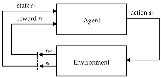
Figure 1.
Agent–environment interaction loop in reinforcement learning.
Different RL methods have proven that they can be effectively used in solving many complex control problems in simulations and real domains. Some agents trained in a simulation domain cannot be easily transferred and used in a real domain. There are problems with modeling different parameters such as friction, mass, tension, and damping. This can be related, for example, to the perception of the environment by the cameras applied in robots. It is not easy to represent these factors as numbers. To tackle this problem, different methods are proposed, for example, sim-to-real techniques based on domain randomization [14], progressive networks [15], and domain adaptation [16]. There are also techniques for minimizing oscillatory movements in robot navigation [17].
In [18], Li gives an overview of the recent, exciting, and important achievements of Deep Reinforcement Learning (DRL). Six core elements and some number of important mechanisms, as well as twelve applications, are discussed. The backgrounds of machine learning, reinforcement learning, and deep learning were explained. In particular, the Deep Q-Network (DQN) and policy, reward, model, planning, etc. were presented. Various applications of DRL such as in games, natural language processing, machine translation, dialogue systems, text generation, computer vision, Industry 4.0, intelligent transportation systems, and robot control are described.
A very interesting application of standard RL algorithms for control of agents that compete in a simple game of hide-and-seek is presented in [19]. In this game, a mixed cooperative and competitive physics-based environment is introduced. In a learning process, only a visibility-based reward function and competition are used. The results showed that agents learned many emergent skills and strategies. It is worth pointing out that they learned the use of collaborative tools and intentionally changed their environment to suit their needs. In the process of learning, the agents created a self-controlling curriculum that contained many distinct rounds of different strategies, many of which required sophisticated tool use and coordination.
In [20], a framework for RL for mobile robots is described. Example trajectories are used in the learning process, which consist of two phases. In the first example, the robot was controlled by an exemplary trajectory for a given task or was controlled directly by an operator. The RL observes the actions, states, and rewards obtained by the robot, and uses this information for the approximation of a value-function. If the learned policy is assessed as acceptable to control the robot, the second phase of learning is used, in which the RL method is used to control the robot. In this step, the Q-learning framework is applied to progress the learning. During the investigations, the robot translation speed is constant. The goal is to lead the robot to its goal point while avoiding obstacles on its path. A reward equal to 1 is used if the robot has reached the goal, and a reward equal to −1 is given if the robot has hit an obstacle. A reward equal to 0 is given in all other cases. The final efficiency obtained did not differ significantly (at the level of 95%) compared to the results obtained with direct robot control.
Mirowski et al. [21] investigated robot navigation ability using the RL algorithm. Task performance is improved by solving a problem of maximizing cumulative reward and jointly considering unsupervised and self-supervised tasks. The authors used two auxiliary tasks: the first for learning obstacle avoidance by unsupervised reconstruction of a simple depth map, and the second for short-term trajectory planning by solving a self-supervised loop closure classification task. The results were validated in complex 3D mazes using raw sensory input. The robot behaved similarly to a human, including when the start and goal locations were changed.
The article [22] describes the use of Twin Delayed Deep Deterministic policy gradient (TD3) to avoid obstacles by a 3-axis robotic arm. The authors compared its operation with the Probabilistic Roadmap (PRM) algorithm. A 90% success rate was achieved for the gain learning algorithm and a 3% shorter motion trajectory compared to the PRM algorithm. However, the algorithm was only implemented in the simulation. The same authors in [23] tested the proposed system in a laboratory on a real robot. Additionally, they implemented Soft Actor Critic (SAC) and Hindsight Experience Replay (HER). Due to various combinations of algorithms, the trajectory was 10% shorter compared to the PRM algorithm.
Wen et al. [24] proposed the use of a DDPG algorithm to plan the trajectory of motion of the Nao robotic arm in simulation. They used the reward function, depending on the target position and the actual position of the manipulator. The agent trained in this way was able to position the TCP (tool center point) of the robotic arm in a given point, but it was not able to avoid obstacles without collision. In order to improve the learning procedure, the authors formulated a reward function that also depends on the distance of the manipulator to the obstacle. The results of simulation tests confirmed that the modified algorithm allowed the robot to successfully avoid obstacles. A similar approach was used by the authors of [25], which also used an RL algorithm called Q-learning to plan the robot’s path and avoid obstacles. The research was performed only in the simulation domain.
Another example of path planning using the RL algorithm was proposed by Bae et al. [26]. Their algorithm combines the RL algorithm with the path planning algorithm of the mobile robot to compensate for the disadvantages of conventional methods by learning the situations where each robot has mutual influence. In most cases, known path planning algorithms are highly dependent on the environment. Other examples of applications of RL methods in mobile robots are presented in [27,28].
In [29], the authors proposed a learning algorithm based on cooperative multi-agent RL to control the Baxter robot. The algorithm was developed using a simulated planar 6-DOF with a discrete action-set. The results showed that all the points reached by the manipulator have an average accuracy of 5.6 mm. The algorithm was found to be repeatable. The authors implemented the concept and tested it on the Baxter robotic arm to obtain accuracy up to 8 mm.
Deep Deterministic Policy Gradient (DDPG) methods have been successfully used in several applications in different robotic control tasks. In [30], the obstacle avoidance and navigation problem in the robotic Unmanned Ground Vehicles (UGVs) control area was investigated. Revised DDPG and Proximal Policy Optimization (PPO) algorithms with improved reward shaping methods are proposed. The performances between these methods were validated in simulation.
Duan et al. in [31] presented a set of continuous control tasks, including the movement of a 3D humanoid robot with partial observations and tasks with a hierarchical structure. They attempted to address the evaluation by presenting a benchmark consisting of 31 continuous control tasks. The authors compared DDPG with batch algorithms, concluding that on certain tasks, DDPG was able to converge significantly faster, but it was less stable than batch algorithms. It was also more susceptible to scaling of the reward.
Gu et al. [32] have demonstrated that the Deep Deterministic Policy Gradient algorithm (DDPG), which is an off-policy deep Q-function-based algorithm, can achieve training times suitable for real robotic systems. Authors have shown in experimental evaluation that this method can teach different 3D manipulation skills, such as door opening, to a real robot any special demonstrations.
In [33], the results of several RL tasks with three commercially available robots are presented. The tasks present different levels of difficulty and repeatability. An experimental study of multiple policy learning algorithms, e.g., TRPO, PPO, DDPG, and Soft-Q, was made. The results showed that these methods can be easily applied to real robots. RL algorithms were also used in other areas of robotics such as pick and place [34], push tasks [35], tossing arbitrary objects [36], and dexterous manipulation of the objects [37,38,39,40,41].
The use of RL methods in the positioning of the robots and avoiding obstacles opens the way to introducing self-learning methods in robot programming and control. The use of the RL algorithm allows a robot to achieve a certain degree of autonomy by learning to move by itself in order to perform a task, e.g., positioning by trying and gathering experience. Thanks to this, a robot can adapt to changes in the environment such as the appearance of an obstacle, which is difficult for classic control methods.
The main contribution of this paper is an RL-based algorithm designed to avoid obstacles and control the positioning of the robotic arm. The authors applied a Deep Deterministic Policy Gradient combined with Hindsight Experience Replay in order to build a multi-agent system to avoid an obstacle and reach the goal position as fast as possible. In order to adapt the algorithms to the task of avoiding obstacles, changes in the operation of the RL algorithms have been made. In case of laboratory investigations to detect the obstacle, a dedicated head with optical (laser) sensors attached to the wrist of the robot was designed and built.
2.2. Algorithms
We selected a combination of state-of-the-art RL algorithms for continuous action space that are often used in different areas of robotics. The authors implemented the algorithms in Python and Tensorflow using the Stable Baselines library [42]. The selected algorithm is Deep Deterministic Policy Gradient (DDPG) [43] combined with Hindsight Experience Replay (HER) [44]. This section briefly describes these two algorithms.
2.2.1. Deep Deterministic Policy Gradient
DDPG is classified as a model-free, off-policy RL algorithm for continuous action spaces that simultaneously learns a Q function and a policy. This algorithm uses the agent, which interacts in discrete time steps with an environment. In every step, the agent receives an observation , performs an action , and receives a reward . The algorithm utilizes the Bellman equation [12] to learn the Q function and utilizes this Q function to learn its policy. DDPG uses four following neural networks: a Q network , a deterministic policy network , a target Q network , and a target policy network . Artificial neural networks are characterized by parameters with superscript that indicates which network it is.
DDPG utilizes also replay buffer in which the experience is stored and samples from it to update the neural networks parameters. During each trajectory rollout, all tuples () of the experience are saved and stored in a finite-sized cache. The parameters of the tuples are: state in time , an action in time , a reward in time , —the next state in time . In order to update the neural network parameters, a random minibatch of tuples () is taken (sampled) from the replay buffer . Subscripts mean that tuples are sampled from the replay buffer as past experience.
The target for the Q network is determined using the following equation:
where is a discount factor in the range 0 and 1; it is usually close to 1. The Q network is trained by minimizing the mean-squared loss between the main Q function and the target :
The policy must derive the action that maximizes ; thus, the policy is updated with a policy gradient using the following formula:
The target network Q is copied from the main network every fixed number of steps. It is updated once per main network update using Polyak averaging:
where .
Noise is added to every action to provide exploration in DDPG with deterministic policy. The time-correlated Ornstein–Uhlenbeck noise [45] is used in the original paper, but later results show that uncorrelated, mean-zero Gaussian noise works superbly. The final action is determined using the following formula in which the noise in time is included:
2.2.2. Hindsight Experience Replay
HER is a buffer of past experiences that allows learning from failures. In [44], authors recommend the following strategy: suppose the agent makes an episode of attempting to reach the goal state starting from the initial state , but fails and ends in some state at the end of the episode. In the HER algorithm, the trajectories are stored into a replay buffer :
where: denotes concatenation; states; actions; rewards.
The idea behind HER comes from human behavior when solving problems, during which humans fail to perform some tasks. In such cases, humans can recognize what has been done wrong and what may be useful to solve the problem. The HER algorithm assumes that target has really been in a state all the time and the agent has reached the goal successfully and received the positive reward . In the control process, the additional trajectory is stored:
This is an imaginary trajectory that arises from the human ability to learn useful behaviors from wrong actions. The reward obtained in the last step of the episode is considered as positive reward obtained for reaching an imaginary goal. By introducing imaginary trajectories into the replay buffer, it is possible to learn how to achieve a goal, even when the applied policy was wrong. This methodology allows the agent to gradually improve the strategy and acquire the target goal more quickly.
2.3. Methodology of the Research
2.3.1. Description of the Robotic System
In order to evaluate the suitability of the described above algorithms for positioning tasks in which it is necessary to avoid obstacles, a robotic system was used and investigated in the laboratory tests. In the research, a complete industrial robot connected to a control computer was used. In the investigations, presented in Figure 2, a simulation model of the robot was used. It was implemented in the virtual environment using the MuJoCo physical engine [46]. This enabled the simulation of the robot and allowed the algorithm to teach the agent to perform the task. The computer used for simulation had the following configuration: CPU: Intel Core i7-8700K; GPU: GeForce RTX 2080Ti. It was working under Linux Ubuntu 18.04 operating system.
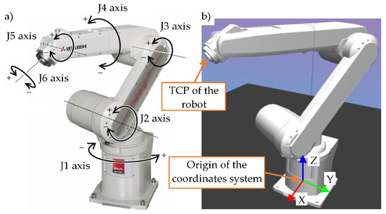
Figure 2.
The Mitsubishi RV-12SDL-12S used in the research: (a) the physical robot with marked joints; (b) the 3D model of the robot in a virtual environment with marked axes X, Y, and Z.
In the investigations, the authors used a 6-DOF robotic arm Mitsubishi RV-12SDL-12S, as shown in Figure 2a. The repeatability precision of this robot is ±0.05 mm. The robotic arm view with marked joints is shown in Figure 2a. The working ranges of the six axes are: J1: [−170°, +170°]; J2: [−100°, +130°]; J3: [−130°, +160°]; J4: [−160°, +160°]; J5: [−120°, +120°]; J6: [−360°, +360°]. The robot drives were equipped with absolute encoders used to measure the current position. The robot controller communicated with the control computer using Ethernet.
2.3.2. Description of a Research Experiment
The goal of the algorithm was to learn to achieve the target position of the TCP of the robot as accurately and quickly as possible. In case of an obstacle, the robot had to avoid it and still achieve the desired position. The robot was working without any payload. At first, the agent was trained in a simulation environment to learn the optimal strategy to ensure the completion of the task. After training the optimal policy in simulation, the strategy was tested on a simulated model of the robot and on the physical robot. The algorithm was trained for 5 × 10⁴ steps. The number of steps was selected so that the value of the reward in the function of the number of steps during the training reaches a plateau—an almost constant, unchanged value. In order to find optimal hyperparameters, we used the OPTUNA hyperparameter optimization framework [47]. Selected hyperparameters of the algorithm are presented in Table A1 in Appendix A.
The observations of the agent creating the state were: current TCP position () in meters; linear velocity of the TCP () in ; target position () in meters; distance of the TCP of the robot from the obstacle in meters; and contact binary information whether any part of the robotic arm has touched an obstacle or not (true/false). The last information was only provided in simulation investigation and helped to teach the agent the kinematics of the robotic arm. Altogether, there are 11 observations. In every step of control, the algorithm generated an action , which is a 3-dimensional TCP displacement described by increments in meters ().
In order to make sure that in the event of an obstacle appearing in the workspace, the robot can bypass it without collision and reach the desired position as quickly and accurately as possible, a special training approach was proposed. The whole process of training was divided into episodes with a fixed maximum number of steps (moves) that the robot can perform. The maximum number of steps for each episode was 50. Each episode during training differed from the others. While the obstacle appeared in the workspace with some chosen probability, the position of the obstacle, the start position of the TCP of the robot, and the goal position were sampled from a uniform distribution. The start and goal positions were sampled from workspace with the following limits, -axis: 0.7 m–1.05 m; -axis: −0.45 m–0.45 m; -axis: 0.6 m–0.9 m. Coordinates of the obstacle position were sampled with the following limits, -axis: 0.85 m–1.05 m; -axis: −0.1 m–0.1 m; -axis: const. Data were given in relation to the robot’s coordinate system-origin (Figure 2b). The workspace in the simulation environment (Figure 3) has the same dimensions as the workspace of the actual robot arm installed in the laboratory. In simulation investigations, the obstacle had a cuboid shape and a size of 0.07 × 0.1 × 1.2 m; in an investigation conducted in the laboratory, Styrofoam blocks were used as obstacles of different sizes. The RL-based algorithm for avoiding obstacles by the robotic arm is presented in Algorithm 1.
| Algorithm 1. RL-based algorithm for avoiding obstacles by robotic arm |
| 1: Initialize neural networks with parameters and , |
| 2: Initialize buffer |
| 3: for episode = 1, do |
| 4: if random_uniform(0, 1) > |
| 5: hide obstacle |
| 6: generate goal position gripper start position from uniform distribution |
| 7: else |
| 8: generate obstacle position |
| 9: generate goal position from uniform distribution #not inside obstacle and not in a forbidden zone near to the obstacle |
| 10: if random_uniform(0, 1) > |
| 11: generate gripper start position on the same side as the goal position # coordinates have the same sign |
| 12: else |
| 13: generate gripper start position on the opposite side of the goal pos. # coordinates have different signs |
| 14: for = 0, − 1 do |
| 15: select action according to the current policy: |
| 16: symbol denotes concatenation |
| 17: execute action and observe new state |
| 18: for = 0, − 1 do |
| 19: |
| 20: store transition in |
| 21: sample a set of additional goals for replay |
| 22: for ∈ do |
| 23: |
| 24: store transition in |
| 25: if update neural networks parameters then |
| 26: sample a random minibatch } from |
| 27: Calculate target |
| 28: |
| 29: update neural network parameters : |
| 30: |
| 31: update neural network parameters |
| 32: J |
| 33: update the target networks: |
| 34: |
| 35: |
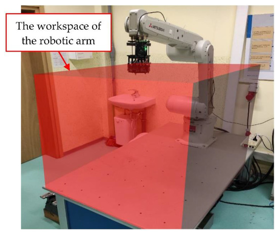
Figure 3.
The workspace of the Mitsubishi robotic marked with a red cuboid.
There are two main parameters in the learning process. The first, is the probability of the presence of the obstacle in the workspace, which is set to 0.9. The second, is the probability that the start position of the robot’s TCP is on the same side of the obstacle as the goal position (signs of the coordinates of the start position of the robot’s TCP and goal position are the same), which is set to 0.1.
The first parameter (line 4—Algorithm 1) is to ensure such a generalization of the environment that, in case of no obstacle nearby the robot, it will move toward the goal along the optimal trajectory (trajectory close to a straight line, without curvation caused by an obstacle). This is done to avoid overfitting. The research has shown that if the first parameter is too small, the robot cannot avoid the obstacle correctly in some cases or even in every case. We believe that in this situation, the agent gained too little experience in avoiding obstacles (learning time did not help to improve it). When the agent is trained in a scenario where the first parameter is too large or even if it is equal to 1 (in all episodes an obstacle appeared), after the learning process the robot tends to move along a non-optimal trajectory, i.e., the robot does not move towards the goal as quickly as possible.
The second parameter (line 10—Algorithm 1) is introduced in order to ensure that the robot could achieve its main objective, which was achieving a specific position in space without interacting with or moving too close to an obstacle. If the is too small, i.e., less than 0.1, the robot is not able to achieve the goal position. The robot does not move towards the goal because when it is too close to the obstacle, the agent receives a larger penalty, which prevents it from exploring the workspace, finding a goal, and thereby obtaining a larger reward after the correct maneuver bypassing the obstacle. In the case when is too larger, the robot cannot learn how to avoid obstacles. During testing, different approaches were tested in order to achieve the desired behavior of the robot. An application of a much more complicated reward function than the one described in Section 2.3.4 does not seem to improve the policy of the agent.
Tests showed that an agent trained in an environment with obstacles to both avoid the obstacles and reach the goal position as quickly as possible, when in an environment without obstacles, does not achieve the target as quickly as possible compared to an agent trained only to achieve the goal position as quickly as possible. To address this problem, the application of two agents working in parallel is proposed. The scheme of such a system is presented in Figure 4. The agent trained to avoid obstacles is called Agent#1 and the agent trained to achieve the goal position as fast as possible moving along an optimal trajectory (trajectory close to a straight line created based on the start and goal position) is called Agent#2.
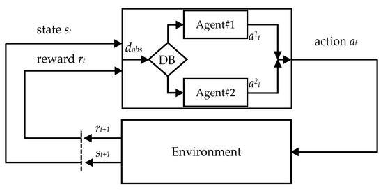
Figure 4.
Multi-agent system.
Observations of Agent#1 are the same as Agent#2. Both agents generated actions as 3-dimensional TCP movements (). During the tests, both agents operate in parallel, and an additional block called the Decision Block (DB) chooses which agent should perform an action in the environment and move the TCP of the robot. DB is simply a conditional statement that, based on the distance between the TCP of the robot and the obstacle, decides which agent should take an action. The threshold distance was set to 0.25 m, i.e., if the distance between the TCP and the obstacle is smaller than this value, Agent#1 takes an action; if the value is larger, Agent#2 does.
We performed research on the simulated model of the robot and on the physical one. For every algorithm, the results obtained in simulation and during deployment on the physical robot were compared for the same 50 start gripper positions and 50 goal positions to ensure a reliable comparison between different attempts at training. As for the position of the obstacle, in the simulation investigation, 50 different, known positions were tested; in laboratory investigation, there were also 50 positions, but they were not the same as in simulation investigation. This was because it is impossible to set the obstacle in the same position as used in simulation and change its position in each episode. During laboratory investigation, an obstacle was placed inside the workspace by the operator. All 50 points were sampled from the uniform distribution in a 3D space box.
The parameters presented and compared in Tables 1 and 2 are the distance (error ) of the robot’s TCP from the target position, standard deviation of the distance (error ), maximum error , and error for different axis , , . Error is calculated from the formula:
where are the difference between the coordinates of the robot’s TCP position in the last (terminal) step of the episode and the goal position.
In order to adapt the algorithms to the task of avoiding obstacles, the authors made changes in the operation of the HER algorithm in terms of storing data in the standard replay buffer (line 20—Algorithm 1) and storing data when creating additional transitions during HER sampling (line 24—Algorithm 1). The new information that is stored in the buffer is the distance of the TCP of the robot from the obstacle and contact binary information . These data are used during the calculation of the reward function in the optimization step of the DDPG algorithm.
2.3.3. Detection of the Obstacle
In the case of simulation investigation, the position of the obstacle is known and it is easy to establish the distance between the TCP of the robot and the obstacle in every step. The obstacle has a cuboid shape; hence, distance is calculated as a distance between the coordinates of the TCP of the robot and the coordinates of the closest point on the surface of the cuboid (obstacle). Therefore, the distance is the smallest distance between the TCP and the obstacle.
In the case of laboratory investigations, determining the distance is not so simple. In order to address this problem, a dedicated head with optical (laser) sensors attached to the wrist of the robot was designed and built. A total number of ten VL53L1 time-of-flight sensors were used (Figure 5a). These sensors measure the time for emitted light to travel from the sensor to the object in front of it and back again. Due to the fact that the speed of light is a constant value independent of changing environmental conditions, such sensors are characterized by high measurement precision independent of the color and the degree of reflection of light of the tested object. The sensor is equipped with an infrared laser of the Vertical-Cavity Surface-Emitting Laser (VCSEL) type with wavelength of 940 nm and a SPAD (Single Photon Avalanche Detector) avalanche photodiode. The field of view of each optical sensor is equal to a 27° cone. The sensors are placed around the ring on the head. Visualization of cones and field of view for every sensor is presented in Figure 6. Even though sensors do not cover all space in front of the head, they are still able to correctly detect obstacles smaller than the human hand. The range of obstacle detection by the head is constrained to 1.5 m. The CAD project of the head is presented in Figure 5a and a photo of the robot with the head is shown in Figure 5b.
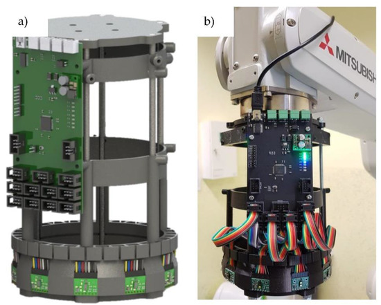
Figure 5.
The head designed to detect obstacles: (a) CAD project; (b) head attached to the wrist of the robot.
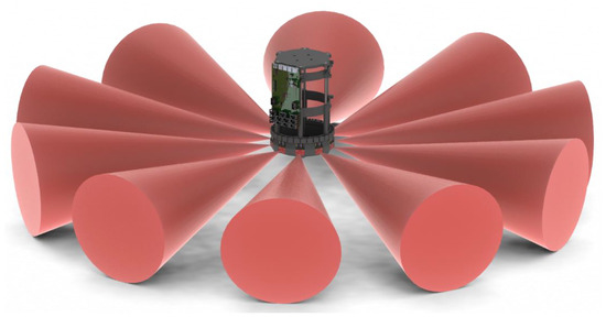
Figure 6.
Visualization of cones and field of view for every VL53L1 time-of-flight sensor.
In order to collect distances from sensors and preliminary data analysis, a PCB with microcontroller STM32F446 was designed and made. The board communicates with the computer via a serial interface—UART-USB. The simple electronic scheme of the board is presented in Figure 7. All data obtained from the sensors are sent to the computer, which analyzes them in order to determine the shortest distance between the head and the obstacle. For the determination of , +the smallest distance transmitted by one of the sensors is selected.
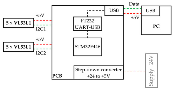
Figure 7.
Electronic diagram of the head.
Due to the time and method of communication of the microcontroller with VL53L1 sensors, to ensure the required sampling rate (15 Hz) of data from VL53L1 sensors, it is necessary to use two separate I2C buses operating in Fast mode. Five VL53L1x sensors are connected to each master bus.
The head that was been built is only a prototype; therefore, its cost is very low and it aims to check whether an investigated method and algorithms can properly work in laboratory conditions using a real robot. Thanks to this, it is possible to verify the results of the simulation tests in reality. The head is designed in such a way that it is possible to extend its functionality and add more sensors. New sensors can be added to the existing ring. An additional ring can also be added in which the sensors are pointing at different angles. The head is empty and it is also possible to insert the gripper. The head can be optimized by taking into account its size.
2.3.4. Reward Functions
Agent#1, which is trained to avoid an obstacle, uses a reward function that takes into account the achieved position , and the goal position . The reward is calculated based on the Euclidean distance between point and point . Additionally, the reward calculation takes into account a parameter , which is a clipped logarithmic distance of the TCP of the robot from the obstacle multiplied by weight obstacle coefficient , which in the investigations is equal to 0.5. To avoid infinite reward during training, while is equal to 0, an additional small number is added in the logarithmic function. Distance is a fixed number that is equal to 0.115 m. It is the distance of the TCP of the robot to the obstacle, from which the is taken into account to reward . The reward is derived using the formula:
Agent#2 is trained in order to achieve the goal position as fast as possible; therefore, it takes into account the optimal trajectory and the trajectory on which the agent moves. The reward is calculated using the equation:
where dtr is the distance between the achieved position and the point that lies on the ideal trajectory (usually a line) based on the start position and target position . The distance is calculated from the formula:
where is the start position, is the goal position, and is the achieved position. Coefficient is a weight coefficient, which represents the extent to which the distance is relevant for calculating the reward . In the investigations, the value of this coefficient is equal to 20.
Combining these two rewards into one equation results in a situation in which the agent is unable to achieve two goals simultaneously (avoiding obstacles and achieving the goal position as fast as possible when an obstacle is not in the workspace) compared to the case of the separate rewards and multi-agent system.
3. Results
3.1. Simulation Results
In Table 1, simulation results characterized by the parameters presented in the previous section for all 50 points are presented. The average position error (the distance between the goal point and the TCP of the robot) is equal to 3.84 mm. Standard deviation for error is equal to 1.83 mm. The maximum error that occurred during testing was over 8 mm in only a single case. The results mainly oscillate around the average error . For individual axes, the greatest error occurred for the axis; it was almost 2.6 mm. The errors for the remaining two axes were below 2 mm.

Table 1.
Results of simulation tests for the task of TCP positioning of the robot at a given point and avoiding an obstacle.
Figure 8 and Figure 9 show the motion trajectories of the robot’s TCP in 2D space recorded during simulation tests. Each figure contains two groups of waveforms: with an obstacle in the workspace of the robot—(a), and without an obstacle—(b). These two panels differ in the presence of obstacles, but are made for the same start position of the TCP of the robot and the same target position. The robot’s trajectories are generated by two agents; therefore, they have two colors; the points marked in purple are actions taken by Agent#1 (labeled as a_obs), and the points marked in cyan are actions taken by Agent#2 (labeled as a_dtr). The presented trajectories include cases in which the starting position of the robot is on both sides of the obstacle on the axis. This means that the coordinate of the start position has a positive and negative sign. During the tests, an obstacle occurred in the workspace after several steps of the entire episode. The obstacle was not in the workspace from the beginning of the episode; it is supposed to simulate the sudden appearance of an obstacle and test the algorithm’s reaction to such a change in the environment.
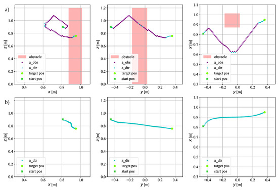
Figure 8.
The trajectory on which the TCP of the robot moved in simulation for goal point : (a) with an obstacle; (b) without an obstacle.
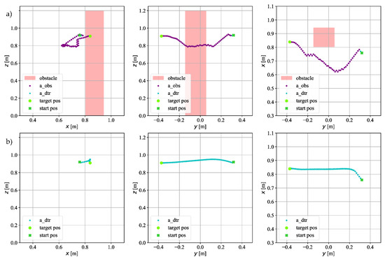
Figure 9.
The trajectory on which the TCP of the robot moved in simulation for goal point : (a) with an obstacle; (b) without an obstacle.
Figure 8 shows the trajectory for the goal position . The coordinate of the starting position has a negative sign. As it can be seen in Figure 8a, at the beginning of the move, the actions are performed by Agent#2 (cyan—a_dtr). After detecting the obstacle, the system switches the agents and the actions are performed by Agent#1 (purple—a_dtr); after a few steps, this agent makes moves to avoid the obstacle that has appeared in the workspace. The agent moves away from the obstacle and then starts moving towards the goal position. It can be seen that during the turning maneuver, Agent#2 takes some steps because the distance between the TCP of the robot and the obstacle has exceeded the threshold distance . After moving away from the obstacle, Agent#2 takes control again, which finally positions the TCP in the goal position. When looking at the -axis graphs, it can be seen that the algorithm does not keep a straight line. At the beginning of the movement, when Agent#1 takes control, it goes up in the -axis, even though the goal point is below the current position of the robot tip. In the case of no obstacle in the workspace (Figure 8b), the task of the agent is to move as quickly as possible towards the goal position. In the figure, some deviation from the straight line can be seen, especially on the axis.
Figure 9 shows the trajectory for the goal position . The coordinate of the starting position has a positive sign. As in the previous case, the first steps are taken by Agent#2; after detecting an obstacle, Agent#1 takes control (Figure 9a). After the turning maneuver when Agent#1 is heading towards the goal position, it turns out that the TCP of the robot is too close to the obstacle. The agent takes additional steps along the obstacle so as to finally avoid it. The goal position is so close to the obstacle that all steps to the end of the episode are taken by Agent#1. Looking at Figure 9b, it can be seen that the agent has not moved in a straight line; the largest deviation from a straight line can be seen again for the -axis.
3.2. Research on the Application of Reinforcement Learning Algorithms to Control a Physical Robot
Similar tests as in the simulation were also carried out on a Mitsubishi robot in laboratory conditions. This robot is shown in Figure 2a and described in Section 2.3.1. In the case of tests carried out in laboratory conditions, different types of objects are used as obstacles, unlike in simulation. In Figure 10, the robot with the mounted head is shown bypassing different obstacles located in its workspace. During tests, robot was bypassing a cuboid block, a cylinder block, multiple obstacles, and a human. Simulation tests and preliminary laboratory tests showed that the size and shape of the obstacle do not affect its detection and avoidance. Therefore, the obstacle dimensions are different than the size and shape of the obstacle used in the simulation.
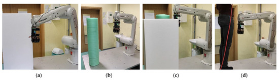
Figure 10.
Mitsubishi robot with the mounted head while avoiding an obstacle: (a) a cuboid block; (b) a cylinder block; (c) multiple obstacles; (d) a human.
In order to compare the simulation outcomes with the tests performed in the laboratory, the algorithm was tested for the same 50 start gripper positions and 50 target positions. This comparison was only carried out with a cuboid block as an obstacle (Figure 10a). In Table 2, results obtained during laboratory investigation are presented. Data presented in this table can be compared with data recorded in simulation, given in Table 1. Comparing Table 1 with Table 2, it can be noticed that the results are very similar. The average error is equal to 3.91 mm, which differs by 0.07 mm compared to simulation tests. Standard deviation for error is higher than in the case of simulation tests and is equal to 2.51 mm. Maximum error is also over 8 mm. For individual axes, the greatest error occurs for the axis; it is 2.69 mm. The errors for the remaining two axes are below 2 mm.
Table 2.
Results of experimental research for the task of robot TCP positioning at a given point and avoiding an obstacle.
Figure 11 and Figure 12 show the example trajectories of the TCP of the robot during tests carried out in laboratory conditions while the robot was bypassing the cuboid obstacle. The method of presentation and the colors of the trajectory fragments performed by Agent#1 and Agent#2 are the same as in the case of figures introduced in the section on simulation tests. In the case of the designed head, the obstacle could not be detected in all three planes, as in the case of the simulation. Therefore, in the figures in Section 3.2, the obstacles are only plotted in the - plane as colored points obtained from sensors. Each laser sensor output signal has a different color; i.e., different colors indicate that the obstacle was detected by another sensor. From this, the shape of the obstacle can be deduced and laser signals used for the detection of an obstacle by the head.
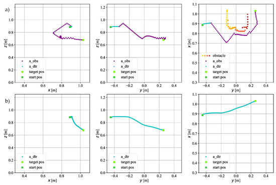
Figure 11.
The trajectory on which the TCP of the robot moved in experimental research for goal point (a) with an obstacle; (b) without an obstacle.
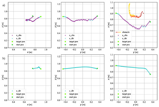
Figure 12.
The trajectory on which the TCP of the robot moved in experimental research for goal point : (a) with an obstacle; (b) without an obstacle.
Figure 11 shows the trajectory for the target point . The coordinate of the start position has a negative sign. As can be seen in Figure 11a, at the beginning of the movement, the actions are performed by Agent#2 because the obstacle is inserted into the workspace when the robot is moving, and not at the very beginning of the episode. The TCP of the robot was too close to the obstacle after performing the turning maneuver; therefore, as can be seen during the simulation tests, Agent#1 moves along the obstacle to avoid it. The goal position is very close to the obstacle; therefore, all steps to reach it are taken by Agent#1. In the case when the obstacle is not in the workspace (Figure 11b), the graphs show that the agent for both the and -axis has a large deviation from the straight line.
Figure 12 shows the trajectory for the target point . The coordinate of the starting position has a positive sign. In this case, oscillations appear, during the obstacle avoidance maneuver, but when the agent passes the obstacle, it begins to move straight to the target without oscillations. When there is no obstacle in the workspace, the deviation from the straight line again occurs for the -axis.
In order to assess whether the algorithm proposed by the authors can avoid obstacles other than the cuboid, additional tests were carried out in which various obstacles, presented in Figure 10, were placed in the workspace of the robot, as mentioned in the introduction to Section 3.2. Figure 13, Figure 14, Figure 15 and Figure 16 show the trajectories of TCP of the robot when there was an obstacle in the shape of a cylinder, two obstacles, and a human.
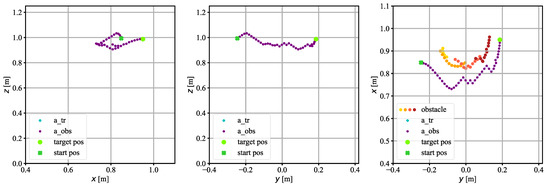
Figure 13.
The trajectory on which the TCP of the robot moved in experimental research. A cylindrical obstacle. Position of the obstacle 0 m.
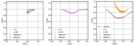
Figure 14.
The trajectory on which the TCP of the robot moved in experimental research. A cylindrical obstacle. Position of the obstacle > 0 m.
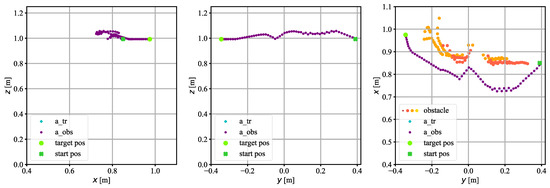
Figure 15.
The trajectory on which the TCP of the robot moved in experimental research. Two obstacles: cuboid-shaped and cylinder-shaped.
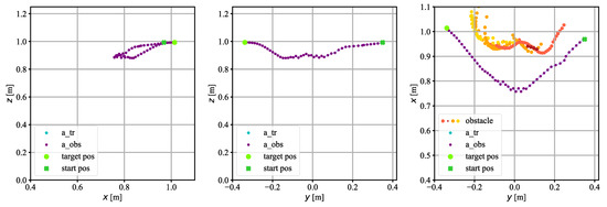
Figure 16.
The trajectory on which the TCP of the robot moved in experimental research. Human as an obstacle.
Figure 13 and Figure 14 show a scenario in which there was a cylinder-shaped obstacle in the workspace of the robot. The obstacles were placed in different places; one of them was placed in the central point of the workspace; i.e., the coordinate of the obstacle was close to 0. The second obstacle was placed in such a way that its coordinate was greater than 0. The algorithm controlled the robot so that it avoided the obstacles without any collisions.
Figure 15 shows the trajectory motion of the robot when a cuboid-shaped obstacle was placed in the workspace, followed by a cylinder-shaped obstacle. At the beginning of the episode, the operator placed the cuboid-shaped obstacle in the workspace, which the robot controlled by the RL-based algorithm avoided without collision. After the avoidance maneuver of the first obstacle, as the robot TCP was moving towards the goal point, a second, cylindrical obstacle was placed in the workspace. This obstacle was also avoided without collision.
Figure 16 shows the trajectory when there was a human in the workspace of the robot. Such an obstacle has an irregular shape, different from those tested before. Its outline registered by sensors in the head is shown on the - plane. In this case, the algorithm had no problem with a collision-free avoidance of the person who entered the workspace of the robot. It can be concluded that the algorithm was able to avoid obstacles of various shapes, both regular and irregular.
4. Discussion
Research conducted in the virtual environment and then validated on the physical robot in the laboratory environment showed that the proposed RL-based algorithm can be used to control a robotic arm to avoid obstacles that dynamically appear in its workspace. The simulation results have shown that the average error e is equal to 3.84 mm. In laboratory investigations, the average error e is almost the same, equal to 3.91 mm. The standard deviation of the error e is 1.83 mm for simulation and 2.51 mm for tests on a real robot. The results obtained in reality are very similar to those obtained during simulation tests. In order to achieve even better accuracy of the positioning, an approach that uses the embedded robot controller for the final positioning of the TCP of the robot can be used. The RL approach can be applied to perform just coarse positioning when the RL agent avoids the obstacle, and when the TCP of the robot is very close to the goal, the embedded robot controller can do fine positioning. In [29], the authors applied RL methods for the positioning task of a robotic arm and in laboratory investigation reached an accuracy of 8 mm, which is almost twice as high as the accuracy of positioning obtained in our research. Furthermore, the algorithm proposed in this article has the ability to avoid obstacles and not only position the TCP of the robot at a target position.
During the tests carried out in the laboratory, the robot performed 100 collision-free obstacle avoidance maneuvers of various shapes dynamically placed in its workspace. Tests conducted on a real robot proved that the algorithm is reliable, which gives a good prognosis for the implementation of the proposed algorithm in the industry, because a large amount of research on obstacle avoidance by robotic arms is still performed only in simulation, e.g., [22,24,25]. Furthermore, the system can be applied to another type of robot due to the integrated obstacle detection system attached to the wrist of the robotic arm, in contrast to the approach in [9], in which the authors tested their algorithm with only one type of an obstacle and used an external camera mounted on a tripod, requiring a computer with better performance comparing to the head with laser sensors.
The proposed approach proved that a domain agent trained in simulation can be implemented to control the real Mitsubishi robot. A trained agent and proposed algorithm can be used to control another type of robotic arm. There is no need for additional training in the case of transfer learning, but the same type of observation introduced in Section 2.3.2 must be provided. The robotic arm must be equipped with a sensor that detects an obstacle and returns the distance in meters in relation to the origin of the robot’s coordinate system. Movements of the TCP of the robotic arm must be also normalized in relation to the origin of the robot’s coordination system.
5. Conclusions
In this paper, the application of a reinforcement learning-based method is proposed to control a 6-axis robot. First, this method and its application in robot obstacle avoidance during the positioning task is described. The Deep Deterministic Policy Gradient and Hindsight Experience Replay algorithms were chosen for the research. We proposed a learning technique and RL-based algorithm for a robotic arm to avoid obstacles. To adapt the RL algorithms to the task of avoiding obstacles, changes in its operations were made. In order to check the usefulness of this algorithm for positioning while ensuring that obstacles are avoided, simulation and experimental tests were carried out with the use of a 6-DOF robotic arm Mitsubishi RV-12SDL-12S. The simulation model of the 6-DOF robot was built in a virtual environment and, first, the agent learned the optimal policy for positioning tasks in simulation. The policy was tested on a virtual model of the robot. To improve the learning process, the application of two agents was proposed. The first agent is trained only to avoid obstacles and the second one is trained to ensure that the robot reaches the goal position as fast as possible. Both agents operate in parallel and receive the same observations; as actions, they generate a 3-dimensional TCP movement (). Distance from the TCP of the robot to the obstacle is the factor that decides which agent should take an action. We conducted tests with various types of obstacles, which were detected by the dedicated head with ten distance laser sensors installed on the robotic arm wrist. Thanks to the application of the RL method, the controlled robot gained a certain degree of autonomy in avoiding obstacles and approaching the target position.
Author Contributions
Conceptualization, T.L. and A.M.; methodology, T.L; software, T.L.; validation, T.L. and A.M; formal analysis, T.L.; investigation, T.L.; resources, T.L. and A.M.; data curation, T.L.; writing—original draft preparation, T.L. and A.M; writing—review and editing, T.L. and A.M; visualization, T.L.; supervision, A.M; project administration, A.M.; funding acquisition, A.M. All authors have read and agreed to the published version of the manuscript.
Funding
Polish Ministry of Science and Higher Education: 0614/SBAD/1565.
Institutional Review Board Statement
Not applicable.
Informed Consent Statement
Not applicable.
Data Availability Statement
Not applicable.
Conflicts of Interest
The authors declare no conflict of interest.
Appendix A
Table A1.
Selected hyperparameters of RL-based algorithm to control the robotic arm.
Table A1.
Selected hyperparameters of RL-based algorithm to control the robotic arm.
| Name | Symbol/Explanation | Value |
|---|---|---|
| action_noise | Ornstein–Uhlenbeck noise 0.434781) | |
| gamma | 0.95 | |
| actor_lr | 0.00037169 | |
| critic_lr | 0.00037169 | |
| batch_size | 256 | |
| buffer_size | 100,000 | |
| rho | 0.999 | |
| Neural network approximating the policy μ | Number of neurons: Activation functions: | [256, 256, 256] [ReLu, ReLu, ReLu] |
| Neural network approximating the function Q | Number of neurons: Activation functions: | [256, 256, 256] [ReLu, ReLu, ReLu] |
| goal_selection_strategy | FUTURE | |
| n_sampled_goal | 8 |
References
- Koubaa, A.; Bennaceur, H.; Chaari, I.; Trigui, S.; Ammar, A.; Sriti, M.-F.; Alajlan, M.; Cheikhrouhou, O.; Javed, Y. Robot Path Planning and Cooperation: Foundations, Algorithms and Experimentations; Studies in Computational Intelligence; Springer International Publishing: Cham, Switzerland, 2018; ISBN 978-3-319-77040-6. [Google Scholar]
- Latombe, J.-C. Robot Motion Planning. Introduction and Overview; SECS; The Springer International Series in Engineering and Computer Science; Springer: New York, NY, USA, 1991; Volume 124, ISBN 978-1-4615-4022-9. [Google Scholar]
- Nakamura, Y.; Hanafusa, H.; Yoshikawa, T. Task-Priority Based Redundancy Control of Robot Manipulators. Int. J. Robot. Res. 1987, 6, 3–15. [Google Scholar] [CrossRef]
- Chiaverini, S. Singularity-Robust Task-Priority Redundancy Resolution for Real-Time Kinematic Control of Robot Manipulators. IEEE Trans. Robot. Autom. 1997, 13, 398–410. [Google Scholar] [CrossRef] [Green Version]
- Iossifidis, I.; Schöner, G. Dynamical Systems Approach for the Autonomous Avoidance of Obstacles and Joint-Limits for an Redundant Robot Arm. In Proceedings of the IEEE International Workshop on Intelligent Robots and Systems, Beijing, China, 9–15 October 2006; pp. 580–585. [Google Scholar]
- Tsetserukou, D.; Kawakami, N.; Tachi, S. Obstacle Avoidance Control of Humanoid Robot Arm through Tactile Interaction. In Proceedings of the Humanoids 2008—8th IEEE-RAS International Conference on Humanoid Robots, Daejeon, Korea, 1–3 December 2008; pp. 379–384. [Google Scholar]
- Khansari-Zadeh, S.M.; Billard, A. A Dynamical System Approach to Realtime Obstacle Avoidance. Auton. Robot. 2012, 32, 433–454. [Google Scholar] [CrossRef] [Green Version]
- Toussaint, M. Robot Trajectory Optimization Using Approximate Inference. In Proceedings of the 26th Annual International Conference on Machine Learning (ICML’09), Montreal, QC, Canada, 14–18 June 2009; ACM Press: Montreal, QC, Canada, 2009; pp. 1–8. [Google Scholar]
- Wei, K.; Ren, B. A Method on Dynamic Path Planning for Robotic Manipulator Autonomous Obstacle Avoidance Based on an Improved RRT Algorithm. Sensors 2018, 18, 571. [Google Scholar] [CrossRef] [PubMed] [Green Version]
- Petrič, T.; Gams, A.; Likar, N.; Žlajpah, L. Obstacle Avoidance with Industrial Robots. In Proceedings of the Motion and Operation Planning of Robotic Systems: Background and Practical Approaches; Carbone, G., Gomez-Bravo, F., Eds.; Springer International Publishing: Cham, Switzerland, 2015; pp. 113–145. [Google Scholar]
- Mahadevan, S. Machine Learning for Robots: A Comparison of Different Paradigms. In Proceedings of the IEEE/RSJ International Conference on Intelligent Robots and Systems (IROS’96), Osaka, Japan, 8 November 1996. [Google Scholar]
- Sutton, R.S.; Barto, A.G. Reinforcement Learning: An Introduction; The MIT Press: Cambridge, MA, USA, 2018. [Google Scholar]
- Kober, J.; Bagnell, J.A.; Peters, J. Reinforcement Learning in Robotics: A Survey. Int. J. Robot. Res. 2013, 32, 1238–1274. [Google Scholar] [CrossRef] [Green Version]
- Peng, X.B.; Andrychowicz, M.; Zaremba, W.; Abbeel, P. Sim-to-Real Transfer of Robotic Control with Dynamics Randomization. 2018 IEEE International Conference on Robotics and Automation (ICRA), Brisbane, QLD, Australia, 21–25 May 2018; pp. 1–8. [Google Scholar] [CrossRef] [Green Version]
- Rusu, A.A.; Vecerik, M.; Rothörl, T.; Heess, N.; Pascanu, R.; Hadsell, R. Sim-to-Real Robot Learning from Pixels with Progressive Nets. In Proceedings of the 1st Annual Conference on Robot Learning, Mountain View, CA, USA, 13–15 November 2017. [Google Scholar]
- Duan, L.; Xu, D.; Tsang, I.W. Learning with Augmented Features for Heterogeneous Domain Adaptation. arXiv 2013, arXiv:1206.4660. [Google Scholar]
- Carmona Hernandes, A.; Borrero Guerrero, H.; Becker, M.; Jokeit, J.-S.; Schöner, G. A Comparison Between Reactive Potential Fields and Attractor Dynamics. In Proceedings of the 2014 IEEE 5th Colombian Workshop on Circuits and Systems (CWCAS), Bogota, Colombia, 16–17 October 2014. [Google Scholar]
- Li, Y. Deep Reinforcement Learning: An Overview. arXiv 2018, arXiv:1701.07274. [Google Scholar]
- Baker, B.; Kanitscheider, I.; Markov, T.; Wu, Y.; Powell, G.; McGrew, B.; Mordatch, I. Emergent Tool Use From Multi-Agent Autocurricula. arXiv 2019, arXiv:1909.07528. [Google Scholar]
- Smart, W.D.; Pack Kaelbling, L. Effective Reinforcement Learning for Mobile Robots. In Proceedings of the IEEE International Conference on Robotics and Automation (Cat. No.02CH37292), Washington, DC, USA, 11–15 May 2002; Volume 4, pp. 3404–3410. [Google Scholar]
- Mirowski, P.; Pascanu, R.; Viola, F.; Soyer, H.; Ballard, A.J.; Banino, A.; Denil, M.; Goroshin, R.; Sifre, L.; Kavukcuoglu, K.; et al. Learning to Navigate in Complex Environments. arXiv 2017, arXiv:1611.03673. [Google Scholar]
- Kim, M.; Han, D.-K.; Park, J.-H.; Kim, J.-S. Motion Planning of Robot Manipulators for a Smoother Path Using a Twin Delayed Deep Deterministic Policy Gradient with Hindsight Experience Replay. Appl. Sci. 2020, 10, 575. [Google Scholar] [CrossRef] [Green Version]
- Prianto, E.; Kim, M.; Park, J.-H.; Bae, J.-H.; Kim, J.-S. Path Planning for Multi-Arm Manipulators Using Deep Reinforcement Learning: Soft Actor–Critic with Hindsight Experience Replay. Sensors 2020, 20, 5911. [Google Scholar] [CrossRef]
- Wen, S.; Chen, J.; Wang, S.; Zhang, H.; Hu, X. Path Planning of Humanoid Arm Based on Deep Deterministic Policy Gradient. In Proceedings of the 2018 IEEE International Conference on Robotics and Biomimetics (ROBIO), Kuala Lumpur, Malaysia, 12–15 December 2018; pp. 1755–1760. [Google Scholar]
- Ji, M.; Zhang, L.; Wang, S. A Path Planning Approach Based on Q-Learning for Robot Arm. In Proceedings of the 2019 3rd International Conference on Robotics and Automation Sciences (ICRAS), Wuhan, China, 1–3 June 2019; pp. 15–19. [Google Scholar]
- Bae, H.; Kim, G.; Kim, J.; Qian, D.; Lee, S. Multi-Robot Path Planning Method Using Reinforcement Learning. Appl. Sci. 2019, 9, 3057. [Google Scholar] [CrossRef] [Green Version]
- Wai, R.-J.; Liu, C.-M.; Lin, Y.-W. Design of Switching Path-Planning Control for Obstacle Avoidance of Mobile Robot. J. Frankl. Inst. 2011, 348, 718–737. [Google Scholar] [CrossRef]
- Duguleana, M.; Mogan, G. Neural Networks Based Reinforcement Learning for Mobile Robots Obstacle Avoidance. Expert Syst. Appl. 2016, 62, 104–115. [Google Scholar] [CrossRef]
- Ansari, Y.; Falotico, E.; Mollard, Y.; Busch, B.; Cianchetti, M.; Laschi, C. A Multiagent Reinforcement Learning Approach for Inverse Kinematics of High Dimensional Manipulators with Precision Positioning. In Proceedings of the 2016 6th IEEE International Conference on Biomedical Robotics and Biomechatronics (BioRob), Singapore, 26–29 June 2016; pp. 457–463. [Google Scholar]
- Zhang, D.; Bailey, C.P. Obstacle Avoidance and Navigation Utilizing Reinforcement Learning with Reward Shaping. arXiv 2020, arXiv:2003.12863. [Google Scholar]
- Duan, Y.; Chen, X.; Houthooft, R.; Schulman, J.; Abbeel, P. Benchmarking Deep Reinforcement Learning for Continuous Control. arXiv 2016, arXiv:1604.06778. [Google Scholar]
- Gu, S.; Holly, E.; Lillicrap, T.; Levine, S. Deep Reinforcement Learning for Robotic Manipulation with Asynchronous Off-Policy Updates. In Proceedings of the 2017 IEEE International Conference on Robotics and Automation (ICRA), Singapore, 29 May–3 June 2017; pp. 3389–3396. [Google Scholar]
- Mahmood, A.R.; Korenkevych, D.; Vasan, G.; Ma, W.; Bergstra, J. Benchmarking Reinforcement Learning Algorithms on Real-World Robots. arXiv 2018, arXiv:1809.07731. [Google Scholar]
- Iriondo, A.; Lazkano, E.; Susperregi, L.; Urain, J.; Fernandez, A.; Molina, J. Pick and Place Operations in Logistics Using a Mobile Manipulator Controlled with Deep Reinforcement Learning. Appl. Sci. 2019, 9, 348. [Google Scholar] [CrossRef] [Green Version]
- Deng, Y.; Guo, X.; Wei, Y.; Lu, K.; Fang, B.; Guo, D.; Liu, H.; Sun, F. Deep Reinforcement Learning for Robotic Pushing and Picking in Cluttered Environment. In Proceedings of the 2019 IEEE/RSJ International Conference on Intelligent Robots and Systems (IROS), The Venetian Macao, Macau, 4–8 November 2019; pp. 619–626. [Google Scholar]
- Zeng, A.; Song, S.; Lee, J.; Rodriguez, A.; Funkhouser, T. TossingBot: Learning to Throw Arbitrary Objects with Residual Physics. arXiv 2019, arXiv:1903.11239. [Google Scholar]
- Kumar, V.; Gupta, A.; Todorov, E.; Levine, S. Learning Dexterous Manipulation Policies from Experience and Imitation. arXiv 2016, arXiv:1611.05095. [Google Scholar]
- Kumar, V.; Todorov, E.; Levine, S. Optimal Control with Learned Local Models: Application to Dexterous Manipulation. In Proceedings of the 2016 IEEE International Conference on Robotics and Automation (ICRA), Stockholm, Sweden, 16–21 May 2016; pp. 378–383. [Google Scholar]
- Andrychowicz, M.; Baker, B.; Chociej, M.; Jozefowicz, R.; McGrew, B.; Pachocki, J.; Petron, A.; Plappert, M.; Powell, G.; Ray, A.; et al. Learning Dexterous In-Hand Manipulation. Int. J. Robot. Res. 2020, 39, 3–20. [Google Scholar] [CrossRef] [Green Version]
- Liu, M.; Hao, L.; Zhang, W.; Chen, Y.; Chen, J. Reinforcement Learning Control of a Shape Memory Alloy-Based Bionic Robotic Hand. In Proceedings of the 2019 IEEE 9th Annual International Conference on CYBER Technology in Automation, Control, and Intelligent Systems (CYBER), Suzhou, China, 29 July–2 August 2019; pp. 969–973. [Google Scholar]
- Añazco, E.V.; Lopez, P.R.; Park, H.; Park, N.; Oh, J.; Lee, S.; Byun, K.; Kim, T.-S. Human-like Object Grasping and Relocation for an Anthropomorphic Robotic Hand with Natural Hand Pose Priors in Deep Reinforcement Learning. In Proceedings of the 2019 2nd International Conference on Robot Systems and Applications, Moscow, Russian, 4–7 August 2019; Association for Computing Machinery: New York, NY, USA, 2019; pp. 46–50. [Google Scholar]
- Hill, A.; Raffin, A.; Ernestus, M.; Gleave, A.; Kanervisto, A.; Traore, R.; Dhariwal, P.; Hesse, C.; Klimov, O.; Nichol, A.; et al. Stable Baselines. Available online: https://github.com/hill-a/stable-baselines (accessed on 14 May 2022).
- Lillicrap, T.P.; Hunt, J.J.; Pritzel, A.; Heess, N.; Erez, T.; Tassa, Y.; Silver, D.; Wierstra, D. Continuous Control with Deep Reinforcement Learning. arXiv 2015, arXiv:1509.02971. [Google Scholar]
- Andrychowicz, M.; Wolski, F.; Ray, A.; Schneider, J.; Fong, R.; Welinder, P.; McGrew, B.; Tobin, J.; Abbeel, P.; Zaremba, W. Hindsight Experience Replay. arXiv 2017, arXiv:1707.01495. [Google Scholar]
- Uhlenbeck, G.E.; Ornstein, L.S. On the Theory of the Brownian Motion. Phys. Rev. 1930, 36, 823–841. [Google Scholar] [CrossRef]
- Todorov, E.; Erez, T.; Tassa, Y. MuJoCo: A Physics Engine for Model-Based Control. In Proceedings of the 2012 IEEE/RSJ International Conference on Intelligent Robots and Systems, Vilamoura-Algarve, Portugal, 7–12 October 2012; pp. 5026–5033. [Google Scholar]
- Akiba, T.; Sano, S.; Yanase, T.; Ohta, T.; Koyama, M. Optuna: A Next-Generation Hyperparameter Optimization Framework. arXiv 2019, arXiv:1907.10902. [Google Scholar]
Publisher’s Note: MDPI stays neutral with regard to jurisdictional claims in published maps and institutional affiliations. |
© 2022 by the authors. Licensee MDPI, Basel, Switzerland. This article is an open access article distributed under the terms and conditions of the Creative Commons Attribution (CC BY) license (https://creativecommons.org/licenses/by/4.0/).