Abstract
The inner-surface damage of water conveyance tunnels is the main hidden danger that threatens their safety and leads to serious accidents. The method based on the principle of acoustic reflection is the main means of inspecting damage to water-conveyance tunnels. However, affected by the tunnel environment and equipment noise, the obtained acoustic point cloud model inevitably suffers from noise, which can produce erroneous results. Therefore, we proposed a novel filtering method, called unsharp-mask-guided filtering for 3D point cloud, to reduce the impact of noise on the acoustic point cloud model of water-conveyance tunnels. The proposed method fuses the ideas of guided filtering and the unsharp masking technique and extends them to the 3D point cloud model by considering the position of the point. In addition, edge-aware weighting mean is also used to retain the edge features of the point cloud model while smoothing the noise points. The experimental results show that our method can obtain impressive results and a better performance in both the acoustic point cloud model of the tunnel and the simulated point cloud model than many state-of-the-art methods.
1. Introduction
Water-conveyance tunnels are the main structures of water-diversion projects. When water-diversion projects enter the operational period, special attention must be paid to the health status of water-conveyance tunnels. The regular inspection of water-conveyance tunnels is an important means of ensuring their safe operation and health management. In recent years, in terms of the problem of tunnel-damage detection, researchers have proposed many methods and technologies (e.g., side-scan sonar, multi-beam sonar, and synthetic-aperture sonar) [1,2,3,4]. The detection method of tunnel damage based on the principle of pulse reflection forms an acoustic point-cloud model by sampling the reflected echo, and then detects and identifies the damage through acoustic point-cloud data [5]. However, affected by the noise of tunnel environments and inspection systems, as well as the noise of carrier equipment (robot carriers and submersibles, etc.), the raw acoustic point-cloud models obtained from these methods inevitably suffer from noise, which makes it difficult to obtain useful information and increases the fuzziness and randomness of information features. In this case, the detection methods that rely on information features produce erroneous results very easily. Therefore, a filtering operation must be performed on the raw acoustic point-cloud model of the tunnel before further processing (e.g., object recognition [6,7] or 3D reconstruction [8]).
Inspired by the excellent results of the guided image-filtering algorithm introduced by He et al. [9], the classical sharpness enhancement technique of unsharp masking [10,11,12] and the edge-aware weighted guided image-filtering algorithm [13], this study extends these effective methods to the point-cloud model of tunnel and proposes a new filtering method, called unsharp-mask-guided filtering for acoustic point-cloud of water-conveyance tunnel, by considering the position of the point instead of the pixel value. The experimental results show that our method can outperform several competing methods (e.g., bilateral filter [14], moving least-squares filter [15], and guided 3D point-cloud filter [16]), both on the acoustic point-cloud tunnel model and the simulated point-cloud model.
The contributions of our work can be summarized as follows: (1) the idea of guided filtering and the unsharp masking technique are fused to design a novel filtering approach for an acoustic point cloud for water-conveyance tunnels; (2) the idea of edge-aware weighting is used to retain the features while smoothing some of the edges of the point cloud; (3) a comprehensively experimental evaluation between our method and several competing denoising methods is conducted on the tunnel point-cloud model and simulated point-cloud model, respectively.
The remainder of this paper is structured as follows. A brief overview of the background and related work is given in Section 2. Section 3 describes the principle and implementation process of our proposed algorithm in detail. The experimental process and experimental results on different point-cloud models are demonstrated in Section 4. Conclusions and discussions are presented in Section 5.
2. Background and Related Work
2.1. Acoustic Point-Cloud Filtering Method
Due to the complexity of underwater environments, the research on the filtering methods of acoustic point clouds, especially the acoustic point-cloud data of water-conveyance tunnels, is limited. Feng et al. [17] proposed a multi-beam point-cloud filtering algorithm that considers the features of underwater terrain. This method is based on the Random Sample Consensus (RANSAC) ideal to fit the local plane, and the coplanar vector feature is used to remove outliers. However, it does not consider that outlier surfaces may be actual obstacles. Xie et al. [18] used the intensity information and elevation information of points to filter the underwater acoustic point cloud. First, a rough classification was carried out according to the intensity information; then, accurate classification and filtering were realized using the intensity information and the elevation information of the seed point and its surrounding points. However, its filtering effect depends entirely on the accuracy of the seed point. Cui et al. [19] studied the combined filtering algorithm of a multi-beam underwater acoustic point cloud. They divided the noise into large-scale and small-scale noise, and then used radius filtering and bilateral filtering, respectively, to achieve point-cloud smoothing. However, this method has the problem of the mistaken deletion of complex terrain. Wang et al. [20] proposed a filtering method that fuses acoustic properties and intensity. They used the filtering method in the process of forming the acoustic point cloud and achieved good results. However, it is not suitable for the filtering of already formed acoustic point-cloud models. Therefore, these studies are not suitable for denoising the acoustic point clouds of water-conveyance tunnels.
By contrast, several studies have been conducted on filtering methods for ground-laser point clouds. Bilateral filtering, originally introduced by Tomasi et al. [21], is a robust edge-preserving filtering method, which has been applied to 3D mesh filtering [22,23,24]. However, these methods need to form mesh models, whose generation process inevitably suffers from noise [25]. Moreover, these methods are always imperfect at retaining the detailed features of point-based data models [26]. In order to overcome this problem, Han et al. [16] proposed an effective point-cloud denoising method by considering the position information of the point. However, in order to reduce the calculation cost, they ignore the fact that the point may be included in different neighborhoods when calculating the conversion coefficient. Therefore, the filtering effect in the acoustic point-cloud model is not ideal and the edge features of the point-cloud model are not well maintained in the smoothing process. Alexa et al. [15] proposed an approach that relies on the idea of implicitly defining a surface for a given set of points. The main idea is to define a projection procedure that projects any point near the point set onto a surface. Next, the MLS (moving least-squares) surface is defined as the set of points projecting onto itself. This method achieves a good smoothing effect, but it smooths the edge features of the point set because of the multiple projection process. Therefore, it is not suitable for surface-feature reconstruction based on the tunnel point cloud.
Currently, most point-cloud filtering methods are based on laser-point cloud data. Owing to the particularity and complexity of the water conveyance tunnel project, the research on acoustic point-cloud filtering methods is limited. Therefore, the acoustic point-cloud filtering methods of water-conveyance tunnels have important practical research value.
2.2. Classical Guided Filtering
Guided image filtering is a well-known time-efficient feature-preserving smoothing operator [9]. The filtered results are obtained by considering the content of the guidance image, and the guidance image can be the input image itself or a different image. This assumes that the filtered output image is a linear transformation of the guidance image in a window. It can transfer the structure of the guidance image to the filtered output, enabling new filtering applications, such as dehazing and feathering. Therefore, guided filtering is essential to the rapid production of edge-feature-preserving denoising applications.
The guided image filtering is given by
where and are the filtered output image and the guidance image, respectively. is the index number of the pixel within window centered at pixel . and are two constants confined to the window . Their values can be calculated by solving
where is a regularization parameter that penalizes large values of and is the original input image. The optimal values of and are calculated by
Here, and are the mean and variance of in , respectively. is the number of pixels in and is the mean of in . To simplify the computation, we assume the guidance image to be the same as the input image [9]. Therefore, we can obtain
According to Equations (1) and (4), the regions with variance () much larger than are preserved, and the regions with variance () much smaller than are smoothed. However, because is a constant in all the neighborhood windows, halos are unavoidable when the filter is forced to smooth some edge features.
2.3. Edge-Aware Weighted Guided Filtering
When the value of a certain pixel at a sharp edge is large, the pixel value in the neighborhood centered on this pixel is affected. The original pixel with a small value becomes larger, and the phenomenon of expansion occurs at the edge. Therefore, the filtered image appears as halo artifacts. If the halo artifacts are not processed, problems such as color distortion and blurred details in the filtered image occur. To overcome the halo artifacts, edge-aware weighted guided image filtering is proposed [13]. It inherits the advantages of both global and local filtering methods in terms that: (1) its complexity is same as that of guided image filtering, and (2) it can avoid halo artifacts such as the currently used global smoothing filters.
Let be the variance of in the window, . An edge-aware weighting is defined by utilizing the local variances of all pixels within a windows. It is given by
Here, is the number of the pixels and is a small constant value to prevent the denominator from being 0. Consequently, they use to perform edge enhancement. The weighting measures the importance of pixel in the overall guidance image. If the pixel is at an edge, the value of is usually larger than 1. Therefore, becomes smaller and in Equation (4) becomes larger. This implies that the sharp edges of in are enhanced.
Unlike the original guided filtering, the value of in edge-aware weighted guided filtering is no longer fixed, but adapts according to the different edge characteristics. Therefore, the edge features can be maintained well while smoothing the image.
2.4. Unsharp Masking
Unsharp masking is a classical sharpness-enhancement technique [12]. The enhancement framework can be summarized as follows. The original image is decomposed into two layers by applying a linear shift-invariant low-pass filter (e.g., the Gaussian filter) [27]. The resulting image is called the base layer, containing the main structure of the original image. The difference produced between the base layer and the original image is called the detail layer, revealing the fine details of the original image. It can be described by
where represents the enhanced image and is the original input image. denotes an unsharp mask, where represents a low-pass filter. controls the effect of enhancement achieved at the output and is the only coefficient to be estimated. Essentially, guided filtering has the same edge enhancement function as unsharp masking by transferring structure from an additional guidance image.
Based on the information above, we derived a novel guided point-cloud denoising formulation from the original guided filter, with the estimation of only one coefficient, akin to the formulation of unsharp masking. To overcome the halo artifacts caused by being a constant value, as described in Section 2.3, an edge-aware weighted method is also proposed to perform edge enhancement while smoothing the edge of the point cloud.
3. Method
Our approach is motivated by the classical sharpness-enhancement techniques of unsharp masking, guided image filtering, and edge-aware weighted guided image filtering. However, these methods cannot be directly applied to 3D point clouds because some point cloud models have only spatial information, and no intensity-attribute information. Therefore, we construct a new widely applicated filtering method by using the position information of points to replace the pixel value in three classical image-filtering methods above. The block diagram of proposed method is shown in Figure 1.
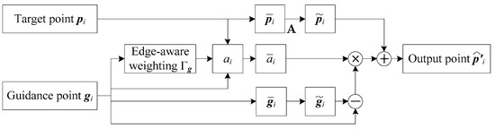
Figure 1.
The block diagram of proposed method.
Given target point-cloud set and guidance point-cloud set , the neighborhood and are searched by using the k-nearest neighbor (KNN) method, where and represent the th neighboring point of and , respectively. As mentioned before, we also assume that the filtered output point cloud has a linear model with the guidance point cloud in a particular neighborhood, that is,
Here, represents the filtered output point of . and are the conversion coefficients in the neighborhood . As with Equation (2) and its optimization solution, we can obtain the values of and by
where represents the number of points in . is a regularization parameter penalizing large . and are the mean and variance of guidance point in . is the mean of in . Taking the calculation of in as an example, it is given by
The filtered output point can be obtained by Equation (7). However, the output point has different values because may be contained in different neighborhoods. Therefore, we calculate the filtered point by averaging all possible values of with
where represents the number of neighborhoods which containing point .
Motivated by unsharp masking, summarized in Equation (6), we insert Equation (9) into Equation (11) to eliminate , and obtain
where , , and .
According to Equation (12), we can more intuitively understand how the unsharp mask guiled filtering achieves edge-preservation and structure-transferring effects. Specifically, the point is smoothed to remove noise and the result is denoted by . Next, to retain the fine details, an unsharp mask with fine features generated from the guide point cloud is added to under the control of the coefficient , enabling the transfer of edge details from the guide point cloud to the filtered-output point cloud.
However, it is clearly visible from Equation (12) that the denoising effect is greatly affected by the number of k-neighborhood points, which determines the values of , , and . If the value of is too large, the resulting point cloud usually loses sharp edges, resulting in over-smoothing problem. Furthermore, if the value of is too small, it cannot achieve the desired denoising effect.
Inspired by the edge-aware weighted guided image-filtering method [13], we introduce the edge-aware mechanism to reduce the impact of edge loss. We use to replace in Equation (8), and is given by
where is a regularization parameter that penalizes large . is a small constant and its value is empirically set as , while is the farthest Euclidean distance between two points in the point-cloud model. is the number of points in the point-cloud model. represents the variance of the point in its k-nearest neighbors and the value of here is selected as 10. When the point is located at a sharp edge, the value of is usually lager than 1 and becomes small. That is, the punishment for in Equation (8) is small and in Equation (12), it is large. Therefore, the fine edge features generated from the guidance point cloud can be maintained well while smoothing noise points.
The results of unsharp mask guided filtering are directly related to the selection of the guidance point-cloud model. Ideally, the ground-truth model without noise should be chosen as the guidance point-cloud model, but this may not be obtained in practical applications. Therefore, we use the raw noisy point cloud as the guidance point cloud. Compared with classical guided filtering, which needs to calculate two parameters , our novel filtering method needs to estimate only one coefficient . At the same time, it can maintain the edge features while smoothing the point-cloud model.
4. Results
Our approach was implemented using MATLAB 2019 on a PC with AMD R5-3500U CPU and 8 GB of memory. We show the results of our method tested on the point-cloud model of a water-conveyance tunnel, and conduct a comparative evaluation with other advanced algorithms. To verify the practicability of the proposed method, we also compared and evaluated the performance of our approach tested on various simulated 3D point-cloud models corrupted with Gaussian noise ranges from 1% to 3% of the diagonal length of the model bounding box. The datasets of the water-conveyance tunnel were derived from the simulated tunnel in the laboratory and the real tunnel on the site. The simulated 3D point-cloud datasets were derived from Large Geometric Models datasets, ModelNet datasets, and ShapeNet datasets [28], respectively.
4.1. Parameters
As introduced in Section 3, the proposed algorithm has two key parameters in addition to the constant parameter and the neighborhood parameter for edge perception. One is the parameter of KNN, which is used to calculate the geometrical neighborhood. For point-cloud models with different numbers of points, the choice of has a great influence on the filtering effect. Another key parameter is , which is a regularization parameter penalizing large . It can simply control the filtering quality. Therefore, we selected a point-cloud model with a different number of points to analyze the impact on the results under different and . The models and parameters used in this experiment are shown in Table 1. Figure 2, Figure 3 and Figure 4 illustrate the results of our method using different values of and , respectively. Table 2 and Table 3 illustrate the quantitative evaluation of the results using the error metric in [29]. When verifying the influence of one parameter on the experimental results, we kept the other parameter constant.

Table 1.
The models and parameters used in experiment.
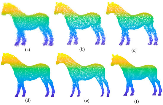
Figure 2.
Filtering results with different values on horse model (). (a) Horse model with noise; (b) filtering result with ; (c) filtering result with ; (d) filtering result with ; (e) filtering result with ; (f) the ground-truth model of horse.
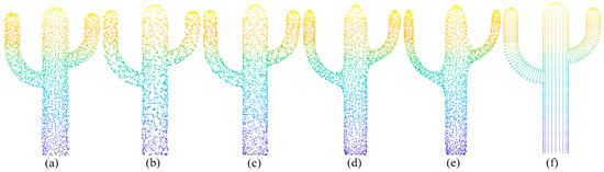
Figure 3.
Filtering results with different values on cactus model (). (a) Cactus model with noise; (b) filtering result with ; (c) filtering result with ; (d) filtering result with ; (e) filtering result with ; (f) the ground-truth model of cactus.
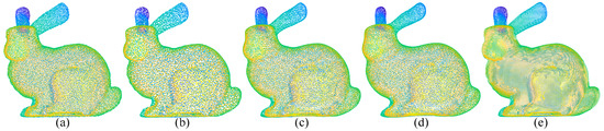
Figure 4.
Filtering results with different values on bunny model (). (a) Bunny model with noise; (b) filtering result with ; (c) filtering result with ; (d) filtering result with ; (e) the ground-truth model of bunny.
Table 2.
Analysis of the results with different values on horse and cactus model. The best results are displayed in bold.
Table 3.
Analysis of the results with different values on bunny model. The best results are displayed in bold.
It can be clearly seen from Figure 2b,c that some noise points may not be removed when is too small. Furthermore, if is too large, as shown in Figure 2e, the point-cloud model shrinks obviously. It is clearly demonstrated in Table 2 that provides the best error-metrics values for the horse model. However, it reveals the different views in Figure 3. The cactus model shrinks obviously when is 50, and the desirable result appears when is 10. It is also demonstrated in Table 2 that provides the best error-metrics values for the cactus model. The reason for the phenomenon of the different values is that the number of points contained in the model and the shape of the model are all different. Furthermore, the choice of is also different under different noise levels.
The second key parameter is , which is a regularization parameter penalizing large . It simply controls the filtering quality. As shown in Figure 4d, if the value of is too large, the filtered results of the bunny model are overly smoothing. Furthermore, if the value of is too small, the excessively large filtering coefficient creates negative effects. It is demonstrated in Figure 4 and Table 3 that provides a desirable result for the point-cloud model of bunny.
Therefore, the parameters of the point-cloud model (e.g., the number of points, the size of the model and shape features, etc.) should be fully considered in order to obtain the desired filtering results. Both of these two parameters need to be adjusted by users according to the experimental requirements and the structural characteristics of the point-cloud model to obtain the best filtering effect.
4.2. Results and Comparison
After a comprehensive analysis of the effect of the parameters in our method, we proceeded to carry out experiments on the point-cloud model of the water-conveyance tunnel and simulated 3D models to compare our algorithm with some state-of-the-art methods, with the aim of exhibiting its performance. In our experiments, we chose three different filtering algorithms, namely, bilateral filter [14], moving least-squares filter [15], and guided 3D point-cloud Filter [16]. Moreover, the results of these algorithms were reproduced on the same computer according to the optimal parameters provided by their authors.
4.2.1. Scene Experiment
The purpose of developing the proposed algorithm is to filter the acoustic point-cloud model of water-conveyance tunnels. Therefore, we conducted an experiment on a real test site to verify the performance of our algorithm. The test site is a small water-conveyance tunnel with a diameter of 80 cm. The ground-truth shape of the tunnel is known. An underwater robot was used as the carrier to collect data [20]. The point-cloud model of the tunnel was corrected by the carrier-attitude information. The raw point-cloud model and the ground-truth model are shown in Figure 5; there are many noise points around the inner surface of the tunnel. In this experiment, we compared the results obtained by the proposed method with the results of the three different filtering algorithms mentioned above.
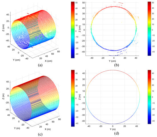
Figure 5.
Raw point-cloud model of water-conveyance tunnel. (a) Raw point-cloud model; (b) front view of (a); (c) the ground-truth model of real water-conveyance tunnel; (d) front view of (c).
Compared with Figure 5a, it is demonstrated in Figure 6a,c,e,g that the four denoising algorithms all achieved the purpose of filtering. This can be more clearly observed in Figure 6b,d,f,h. For the small-scale noise points near the inner surface of the tunnel, it is clearly visible in Figure 6b that the guided 3D point-cloud filter achieved poor effects in smoothing the small-scale noise points. As shown in the blue circular dotted-line area in Figure 6d,f, the bilateral filter and the moving least-squares filter had the problem of over-smoothing while filtering the noise points. Figure 6h demonstrates that the proposed method can prevent over-smoothing while filtering out small-scale noise points. For large-scale noise far away from the inner surface of the tunnel, none of the three methods achieved a good result. By contrast, the results of the proposed method are better than other those of the other three algorithms.
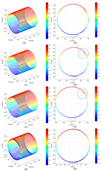
Figure 6.
The results of different algorithms tested on the point-cloud model of water-conveyance tunnel. (a) The result of guided 3D point-cloud filter; (b) front view of (a); (c) the moving least-squares filter results; (d) front view of (c); (e) the bilateral filter results; (f) front view of (e); (g) the results of proposed algorithm ( and ); (h) front view of (c).
To quantitatively evaluate the denoising results, four error-metrics, , , , and , were used in our experiment. represents the average distance between the points in the resulted point-cloud and the corresponding points in the ground-truth model [29]. represents the variance of the distance. is the average radius of the filtered point-cloud model of the tunnel. represents the reconstruction accuracy of the point-cloud model of the water-conveyance tunnel. The calculation results of the error metrics are shown in Table 4.
Table 4.
Analysis of the results of different algorithms tested on the point-cloud model of water-conveyance tunnel (the best results are displayed in bold).
In Table 4, the best results are displayed in bold. It is clearly demonstrated that the results of our method were the best in and . In other words, the filtered points were close to the inner surface of the tunnel and had good aggregation properties. The results of the proposed method also have high accuracy in and . Moreover, it is clearly seen from that the point-cloud model of the real tunnel obtained by the proposed method has a high reconstruction accuracy, which provides important support for defects detection on the tunnel surface.
4.2.2. Simulation Experiment
To verify the applicability of the proposed method, we also executed our algorithm on a simulated model of the water-conveyance tunnel and nine simulated 3D point-cloud models with different shapes and sizes to highlight the advantages. Affected by the noise of the electronic components of the acquisition equipment, the acquired point-cloud model is easily polluted by noise that obeys the Gaussian distribution. Therefore, the Gaussian noise generated using a zero-mean Gaussian function with a standard deviation was added to the simulated 3D point cloud models. The Gaussian noise ranges were from 1% to 3% of the diagonal length of the model bounding box.
As shown in Figure 7, the results of the guided 3D point-cloud filter, moving least-squares filter, and bilateral filter are poor, and there are many noise points around the tunnel. The bilateral filtering results were relatively smooth, but the denoising effect was not perfect, and the tunnel outline experienced distortion. Comparing the inner part of the red rectangle in Figure 7b–e, the denoising effects of the model obtained by the proposed algorithm were much better than those obtained by the other three methods, and the denoising effect of the outliers was obvious. The filtered point-cloud model was closer to the real cylindrical container. The method proposed in this study has an obvious suppressive effect on the outliers while preserving the contour.
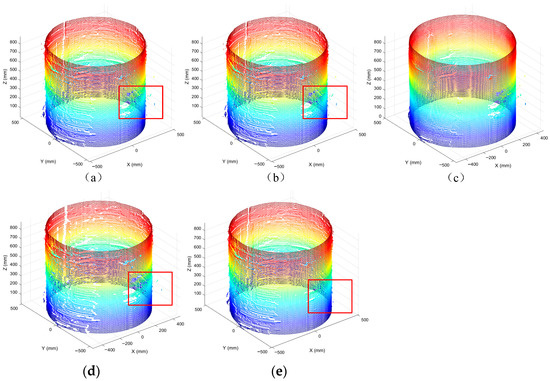
Figure 7.
The results of different algorithms tested on the point-cloud model of simulated water-conveyance tunnel. (a) The original point-cloud model of the simulated tunnel; (b) the guided 3D point-cloud filter results; (c) the bilateral filter results; (d) the moving least-squares filter results; (e) the results of proposed algorithm ( and ).
We also used the error metrics , , , and to quantitatively evaluate the denoising results. As shown in Table 5, the metrics of the moving least-squares filter and bilateral filter were similar. Furthermore, the metrics of the guided 3D point-cloud filter were all poor. The four error metrics of the other three methods were all larger than those of the proposed algorithm. This means that the reconstruction accuracy of the point-cloud model obtained using these methods is poor. By contrast, our method is better than the other three methods in terms of the error metrics, which reflects the superiority of our algorithm.
Table 5.
Analysis of the results of different algorithms tested on the point-cloud model of simulated water-conveyance tunnel (the best results are displayed in bold).
Figure 8, Figure 9 and Figure 10 are the filtering results of the unsharp-mask-guided filtering and several competing methods. Here, we only present pictures of the block, chair, and elephant models. Moreover, the results of these comparison algorithms were obtained according to the optimal parameters provided by their authors. It is clearly visible in Figure 8e that our algorithm can preserve the edge features well without shrinkage or deformation in the block model, while the results of the moving least-squares filter were deformed. For the 3D point-cloud model of the chair, it is shown in Figure 9b,d that the results of the guided 3D point-cloud filter and moving least-squares filter were poor. Moreover, the results of the bilateral filter were deformed. As shown in Figure 9e, the proposed method achieves more satisfactory results with the chair model. For the 3D point-cloud model of the elephant, it is shown in Figure 10 that the comparison methods all achieved satisfactorily smooth results, except for the blurring problem at the mouth of the elephant. It is clearly shown in the enlarged map in Figure 10e that our method can preserve the local feature information of the elephant’s mouth while smoothing the noise points. Furthermore, our method also achieved satisfactory results in six other, different, 3D point-cloud models, according to the values of the error metrics shown in Table 6.
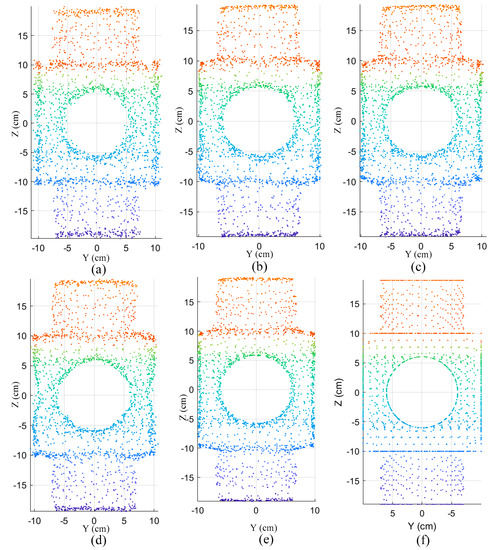
Figure 8.
The results of different algorithms tested on block model. (a) Block model with noise; (b) the guided 3D point-cloud filter results; (c) the bilateral filter results; (d) the moving least-squares filter results; (e) the results of proposed algorithm ( and ); (f) the ground-truth model of block.
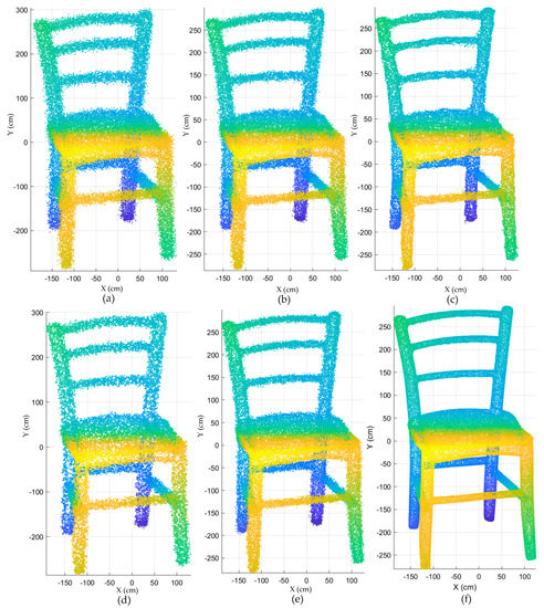
Figure 9.
The results of different algorithms tested on chair model. (a) Chair model with noise; (b) the guided 3D point-cloud filter results; (c) the bilateral filter results; (d) the moving least-squares filter results; (e) the results of the proposed algorithm ( and ); (f) the ground-truth model of chair.
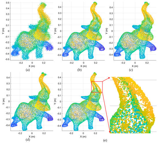
Figure 10.
The results of different algorithms tested on elephant model. (a) Elephant model with noise; (b) the guided 3D point-cloud filter results; (c) the bilateral filter results; (d) the moving least-squares filter results; (e) the results of proposed algorithm ( and ).
Table 6.
Error metrics for different methods and the best results are displayed in bold.
We also used the error metrics and to quantitatively evaluate the filtering results of the different methods. The error metrics for nine different models are shown in Table 6, and the best error-metrics values are highlighted in bold. According to these values, as expected, it is evident that the proposed method obtain better denoising results on most simulated 3D point-cloud models, with the exception of the elephant model. Although the best error-metric values were not obtained on the point cloud-model of the elephant, it can be seen in Figure 10e that our method achieved satisfactory results in maintaining the feature details of the elephant’s mouth. The denoising effect of the bilateral filter in the point-based model was mainly reflected in the smooth effect of the point-cloud model. Furthermore, the error metrics and reflect the overall performance of the resulting model rather than the local detailed properties. Therefore, in our study, there was better error measurement and poor detail-feature retention, such as the elephant’s mouth shape. This also reflects the compromise strategy adopted by the proposed method, which preserves the details as much as possible while maintaining the denoising effect. Overall, the experimental results show that our method is effective on simulated 3D point models, and can ensure the features are more accurate while obtaining smoother filtering results.
The proposed method can achieve more satisfactory results on real site models and simulated models than many other competing methods. And the model obtained by our method is more suitable for the subsequent object recognition or 3D reconstruction tasks of water-conveyance tunnel.
5. Conclusions and Discussion
To address the safety-monitoring problem of a water-conveyance tunnel during the operation stage, we proposed a novel filtering method, called unsharp-mask-guided filtering for 3D point cloud, to reduce the impact of noise on the point-cloud model of the water-conveyance tunnel. The proposed method fuses the ideas of classical guided filtering and the unsharp masking technique and extends them to the 3D point-cloud model by considering the position of the point. In addition, an edge-aware weighting idea was also used to retain the edge features of the point-cloud model while smoothing the noise points.
In the experiment, we examined the influence of two key parameters on the experimental results. We also carried out experiments on real-world 3D models of the tunnel and nine simulated 3D models to compare our algorithm with some state-of-the-art methods. The experimental results show that the proposed method can outperform several competing methods, both on the real-tunnel point-cloud model and simulated point-cloud models. The model provides greater accuracy for the further processing of point clouds. However, we did not consider the efficiency of our algorithm in the experiment. Because our method needs to search the neighborhood twice for each point and to judge the inclusion relationship between the neighborhoods of different points, it does not have an obvious advantage in efficiency. The running time of point-cloud models with different number of points is different. Taking the Stanford rabbit model as an example, the time cost of our algorithm on the hardware device based on this study is 7.2 s, while the time costs of bilateral filtering, MLS filtering, and guidance filtering are 4.5 s, 4.8 s, and 3.7 s, respectively. These time costs are all higher than those in the references because of the weak processing power of the computer equipment used in this study. Therefore, we need to optimize the calculation method to improve the efficiency of the proposed algorithm in future work.
Author Contributions
Conceptualization, J.W. and X.Z.; methodology, J.W.; software, J.W.; validation, J.W., X.Z. and Z.Z.; formal analysis, J.W.; investigation, J.W.; resources, X.Z.; data curation, J.W.; writing—original draft preparation, J.W.; writing—review and editing, J.W.; visualization, J.W.; supervision, X.Z.; project administration, X.X.; funding acquisition, X.Z. All authors have read and agreed to the published version of the manuscript.
Funding
This research was funded by National Key R&D Program of China, grant number 2018YFC0407101, and National Natural Science Foundation of China, grant number 61671202.
Institutional Review Board Statement
Not applicable.
Informed Consent Statement
Not applicable.
Data Availability Statement
The data presented in this study are available from the corresponding author upon request.
Acknowledgments
The authors would like to thank all the reviewers for their valuable comments. We would like to thank Georgia Tech for their Large Geometric Models. We are grateful to Princeton ModelNet project for sharing the ModelNet datasets. We also thank the researchers at Princeton, Stanford, and TTIC for sharing the ShapeNet datasets.
Conflicts of Interest
The authors declare no conflict of interest.
References
- Zhu, X.; Wang, T.; Liu, Y.; Huang, T. A new defect detection technology for long-distance water conference tunnel. Water Resour. Hydropower Eng. 2010, 41, 78–81. [Google Scholar] [CrossRef]
- Liao, J.; Yue, Y.; Zhang, D.; Tu, W.; Cao, R.; Zou, Q.; Li, Q. Automatic Tunnel Crack Inspection Using an Efficient Mobile Imaging Module and a Lightweight CNN. IEEE Trans. Intell. Transp. Syst. 2022, 1–14. [Google Scholar] [CrossRef]
- Jitao, L.; Gande, L. Study on long-term operation safety detection technical system of large and long diversion tunnel. Water Resour. Hydropower Eng. 2021, 52, 162–170. [Google Scholar] [CrossRef]
- Jin, H.; Yuan, D.; Zhou, S.; Zhao, D. Short-Term and Long-Term Displacement of Surface and Shield Tunnel in Soft Soil: Field Observations and Numerical Modeling. Appl. Sci. 2022, 12, 3564. [Google Scholar] [CrossRef]
- Wang, J.; Wang, C.; Han, Z.; Jiao, Y.; Zou, J. Study of hidden structure detection for tunnel surrounding rock with pulse reflection method. Measurement 2020, 159, 107791. [Google Scholar] [CrossRef]
- Park, J.; Kim, H.; Tai, Y.-W.; Brown, M.S.; Kweon, I. High quality depth map upsampling for 3D-TOF cameras. In Proceedings of the 2011 International Conference on Computer Vision, Barcelona, Spain, 6–13 November 2011; pp. 1623–1630. [Google Scholar]
- Zheng, W.; Xie, H.; Chen, Y.; Roh, J.; Shin, H. PIFNet: 3D Object Detection Using Joint Image and Point Cloud Features for Autonomous Driving. Appl. Sci. 2022, 12, 3686. [Google Scholar] [CrossRef]
- Rangel, J.C.; Morell, V.; Cazorla, M.; Orts-Escolano, S.; García-Rodríguez, J. Object recognition in noisy RGB-D data using GNG. Pattern Anal. Applic. 2017, 20, 1061–1076. [Google Scholar] [CrossRef] [Green Version]
- He, K.; Sun, J.; Tang, X. Guided Image Filtering. IEEE Trans. Pattern Anal. Mach. Intell. 2013, 35, 1397–1409. [Google Scholar] [CrossRef]
- Ye, W.; Ma, K.-K. Blurriness-Guided Unsharp Masking. IEEE Trans. Image Processing 2018, 27, 4465–4477. [Google Scholar] [CrossRef]
- Deng, G. A Generalized Unsharp Masking Algorithm. IEEE Trans. Image Processing 2011, 20, 1249–1261. [Google Scholar] [CrossRef]
- Polesel, A.; Ramponi, G.; Mathews, V.J. Image enhancement via adaptive unsharp masking. IEEE Trans. Image Process. 2000, 9, 505–510. [Google Scholar] [CrossRef] [PubMed] [Green Version]
- Li, Z.; Zheng, J.; Zhu, Z.; Yao, W.; Wu, S. Weighted Guided Image Filtering. In IEEE Transactions on Image Processing; IEEE: Toulouse, France, 2015; Volume 24, pp. 120–129. [Google Scholar] [CrossRef]
- Digne, J.; de Franchis, C. The Bilateral Filter for Point Clouds. Image Processing Line 2017, 7, 278–287. [Google Scholar] [CrossRef] [Green Version]
- Alexa, M.; Behr, J.; Cohen-Or, D.; Fleishman, S.; Levin, D.; Silva, C.T. Computing and rendering point set surfaces. IEEE Trans. Vis. Comput. Graph. 2003, 9, 3–15. [Google Scholar] [CrossRef] [Green Version]
- Han, X.-F.; Jin, J.S.; Wang, M.-J.; Jiang, W. Guided 3D point cloud filtering. Multimed Tools Appl. 2018, 77, 17397–17411. [Google Scholar] [CrossRef]
- Feng, D.; Shi, B.; Xiushan, L.U.; Guoyu, L.I. A Multi-Beam Point Cloud Denoising Algorithm Considering Underwater Topographic Features. J. Geomat. Sci. Technol. 2017, 34, 364–369. [Google Scholar]
- Xie, Q.; Tian, M.; Feng, C.; Yu, J.; Pang, Y. Study on Filtering Algorithm Combining Multibeam Point Cloud Intensity and Elevation Information. Hydrogr. Surv. Charting 2021, 1, 65–69. [Google Scholar] [CrossRef]
- Cui, X.; Shen, W.; Shuai, C.; Hui, X. Preliminary research and application analysis ofmulti-beam point cloud filtering algorithm. Hydrogr. Surv. Charting 2021, 5, 12–16. [Google Scholar] [CrossRef]
- Wang, J.; Zhang, X.; Xu, X.; Zhang, Z.; Song, K. Remote inspection method for water conveyance tunnel based on single-beam scanning sonar. JARS 2022, 16, 024522. [Google Scholar] [CrossRef]
- Tomasi, C.; Manduchi, R. Bilateral filtering for gray and color images. In Proceedings of the Sixth International Conference on Computer Vision (IEEE Cat. No.98CH36271), Bombay, India, 7 January 1998; pp. 839–846. [Google Scholar]
- Fleishman, S.; Drori, I.; Cohen-Or, D. Bilateral mesh denoising. ACM Trans. Graph. 2003, 22, 950–953. [Google Scholar] [CrossRef]
- Lee, K.-W.; Wang, W.-P. Feature-preserving mesh denoising via bilateral normal filtering. In Proceedings of the Ninth International Conference on Computer Aided Design and Computer Graphics (CAD-CG’05), Hong Kong, China, 7–10 December 2005. [Google Scholar]
- Jones, T.; Durand, F.; Desbrun, M. Non-Iterative, Feature-Preserving Mesh Smoothing. ACM Trans. Graph. 2003, 22, 943–949. [Google Scholar] [CrossRef]
- Manzo, M.; Rozza, A. DOPSIE: Deep-Order Proximity and Structural Information Embedding. Mach. Learn. Knowl. Extr. 2019, 1, 684–697. [Google Scholar] [CrossRef] [Green Version]
- Zaman, F.; Wong, Y.P.; Ng, B.Y. Density-Based Denoising of Point Cloud. In Lecture Notes in Electrical Engineering, 9th International Conference on Robotic, Vision, Signal Processing and Power Applications; Springer: Singapore, 2017; pp. 287–295. [Google Scholar] [CrossRef] [Green Version]
- Shi, Z.; Chen, Y.; Gavves, E.; Mettes, P.; Snoek, C.G.M. Unsharp Mask Guided Filtering. IEEE Trans. Image Process. 2021, 30, 7472–7485. [Google Scholar] [CrossRef] [PubMed]
- The Stanford 3D Scanning Repository. Available online: http://www.graphics.stanford.edu/data/3Dscanrep/ (accessed on 17 June 2022).
- Han, X.-F. Research on Denoising Processing and Feature Description for 3D Point Cloud. Ph.D. Thesis, Tianjin University, Tianjin, China, 2019. [Google Scholar]
Publisher’s Note: MDPI stays neutral with regard to jurisdictional claims in published maps and institutional affiliations. |
© 2022 by the authors. Licensee MDPI, Basel, Switzerland. This article is an open access article distributed under the terms and conditions of the Creative Commons Attribution (CC BY) license (https://creativecommons.org/licenses/by/4.0/).