Investigation of an Inline Inspection Method for the Examination of Cylinder-like Specular Surfaces Using Deflectometry

Abstract

An optical measuring method is presented, with which it is possible to measure and evaluate reflective cylindrical surfaces using a combination of deflectometry and subsequent reconstruction of the surface. The system is set up and tested on rolling elements of cylindrical roller bearings. However, it is not limited to this use case and can be applied to other cylindrical specular surfaces. The system distinguishes itself from existing test methods through the combination of high-resolution three-dimensional defect measurement with a very short recording time, and offers the possibility of introducing tolerance limits in the production of cylindrical specular surfaces. With this method, it is possible to record a defect with the dimensions of $1.3$ $\mathrm{m}$$\mathrm{m}$ by $1.8$$\mathrm{m}$ $\mathrm{m}$ within 5 $\mathrm{s}$ and to reconstruct the absolute depth. The resolution of the system is below 10 μ$\mathrm{m}$ in both X- and Y-direction, and is therefore sufficiently accurate to detect typical surface defects such as scratches, dents, or deformations. To validate the measured values of the system, the results of an artificially generated $10.35$ μ$\mathrm{m}$ deep defect location were compared with those of a highly accurate mechanical stylus measurement.

1. Introduction

In today’s industry, the demands for manufactured products continue to increase. Primarily, flawless quality is demanded at low prices and high quantities. Therefore, to meet these requirements, a one hundred percent inline inspection of the manufactured parts is desirable in most cases. In many applications, a system from the field of automatic optical inspection is used [1,2]. Since inline inspection systems are often limited to a two-dimensional inspection, in this work, a system was developed which optically extracts three-dimensional information of a cylindrical surface. This additional information can then be used to realize tolerance limits in production. This is mainly applicable to metallic or reflective surfaces [3]. The rolling elements of a cylindrical roller bearing are an example of a cylindrical reflective surface. These bearings are widely used in both the automotive and engineering industries. Although the manufacturing process of the rolling elements in the bearing is highly optimized, a defect in the production of these rolling elements can lead to undesirable quality losses due to the constantly increasing requirements. These defects are often described by the term rolling contact fatigue, and play a major role in material research for bearings [4,5]. Parallel to defects that only occur in the later stages of a bearing’s life, undesirable quality degradation, including bearing failure, also occurs in new bearings. Defects in bearing have a wide range of effects. Most importantly, they lead to undesirable vibrations of the bearing and, because of increasing forces, faster material fatigue [6,7]. These undesired vibrations are often analyzed during the life of a bearing to provide information about its condition [8,9,10]. To avoid the aforementioned problems at an early stage, the idea of this work is to develop a low-cost inline inspection method with a short inspection time for the surface of rolling elements, which detects defect spots and deformations caused by production before the bearing is finally assembled. The system is expected to distinguish from existing inspection systems by extracting three-dimensional surface information with a very short acquisition time. For this purpose, the work of Prappacher et al. [11] is extended. The recording mechanism and the illumination device presented here are used to extract and subsequently reconstruct the surface information with the use of additional techniques presented in the literature.

2. Materials and Methods

2.1. State of the Art

The most established systems for inspecting metallic surfaces rely on the approach of non-destructive eddy current technology [12,13,14]. These eddy current inspection systems induce a current into the metallic material via a magnetic field. Defects, such as scratches or air pockets near the surface, interfere with the current signal and can be detected. These systems can be used on all ferromagnetic components for quality assurance. They have a high inspection speed and good resolution. Furthermore, non-destructive testing methods that use ultrasonic to examine the entire body are presented in [15,16,17]. Since ultrasonic can penetrate into a test specimen, these methods are not limited to pure surface inspection, but also consider defects, such as air pockets in the material. Specifically for the inspection of rolling element surfaces, methods [18,19] can be found in the literature which are limited to two-dimensional surface inspection. Non-destructive optical methods that do not specifically relate to the inspection of rolling elements are also presented. For example, [20,21] point out an optical method that obtains and evaluates two-dimensional surface information via an optical approach. The problem of surface inspection is limited in many systems to the extraction and evaluation of two-dimensional surface information. Thus, in a potential test procedure, a distinction can only be made between good and bad parts. However, since large quantities of parts must be inspected and evaluated in rolling element inspection, the introduction of a tolerance limit would be desirable here to reduce scrap. Thus, an inspection system must also record and evaluate the depth, i.e., three-dimensional information of the defect location. Several approaches to surface inspection exist in the literature. Ideas, such as [22,23] gather under the term of phase-measuring deflectometry (PMD). Here, a stripe-like pattern is observed through the reflective surface of the test object. Changes in this pattern can then be evaluated to conclude the surface condition. However, these approaches are difficult to transfer to the use of a line scan camera for cylindrical surfaces imaging. Other approaches such as [24,25] use Fourier transform profilometry (FTP) to extract surface information. Again, a fringe pattern is used, but this time it is projected onto the surface. The image captured by a camera is then evaluated using this pattern. Two problems arise here. First, projection onto a reflective surface is not possible, and second, the use of a line scan camera to capture the cylindrical surface is not viable. Other ideas such as [26] use interferometry to scan the surface. These methods take a small sized area of the surface with a very accurate depth resolution. Depending on the sampling time of the system, high acquisition times preclude its application as an inline system. The method from work [27] uses different illumination patterns to determine the reflection direction between the camera and screen. This method requires a reflective surface and can also be applied using a line scan camera. A version adapted for line scan cameras will find its application in this work. To evaluate and display this information, the resulting gradient field has to be transformed into a height map, i.e., into a virtual surface. In the works [28,29,30,31,32,33,34] approaches can be found which make this possible.

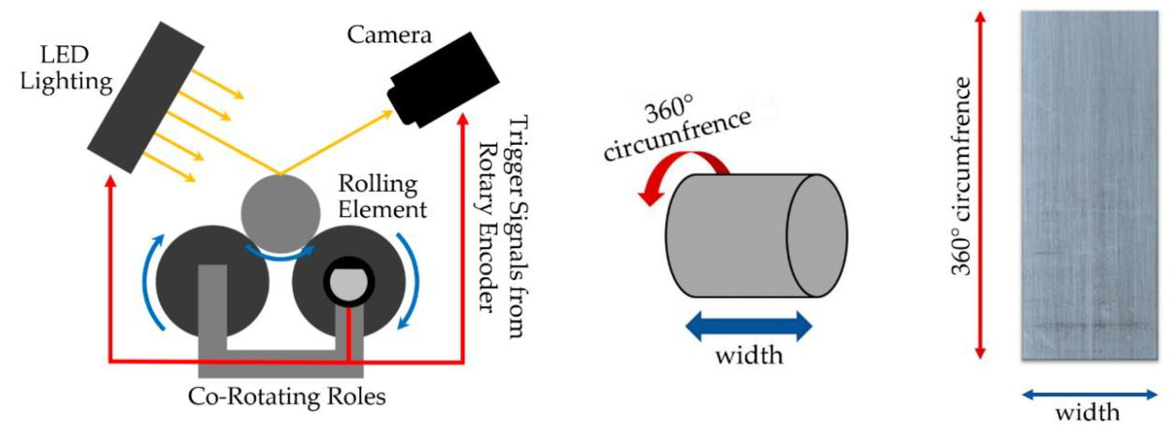
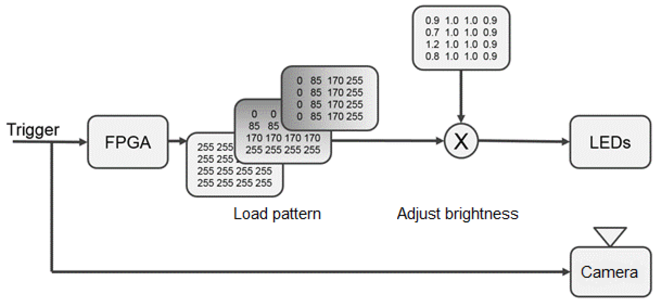
2.2. Hardware

To accommodate the cylindrical rolling element surface, a recording mechanism was implemented in previous work [11] especially for this application. The mechanism is shown schematically in the following Figure 1.

As can be seen, the rolling elements are pushed onto two rotating rollers by a conveyor system. On these rollers, they are rotated to record the circumferential surface of the rolling element cylinder using a line scan camera. In the deflectometric methods from the literature, which use a static illumination pattern, LCD monitors are often used as illumination units. However, these monitors cannot be used in this project because their maximum switching frequency of 140 $\mathrm{Hz}$ is insufficient to image the rolling element’s lateral surface at an acceptable rate. Due to this problem, an illumination unit based on the Xiling Artix 7 FPGA chip was developed. With the help of the FPGA, 200 LEDs arranged in a matrix can be controlled in their lighting duration and intensity with a system clock of 150 $\mathsf{\mu }$$\mathrm{s}$. To be able to switch each LED specifically, a circuit board was developed which contains a MOSFET circuit for each of the 200 LEDs. The resulting 200 galvanically isolated input pins of the driver board are connected to the GPIOS of the FPGA chip to enable it to switch the LEDs quickly and reliably. The intensity of the LEDs is determined in the software by the ratio of the duty cycle of the LED and the exposure time of the camera. To ensure a synchronous sequence in the image acquisition, a rotary encoder is used as a trigger. This encoder is connected to the two rotating rollers on which the rolling elements rotate. The output signal of the encoder is converted by a frame grabber into a trigger signal for both camera and lighting. For each encoder output signal, trigger signals are sent according to the number of illumination patterns. For each trigger signal, the schematic sequence described in Figure 2 is executed.

The incoming trigger signal is processed by both the FPGA and the camera. The FPGA board successively loads one of the exposure patterns for each trigger and performs a homogenization of the brightness. After that, the FPGA board triggers the corresponding LEDs. The camera starts the exposure when a trigger signal arrives. With this sequence, it is possible to ensure that each line, i.e., each output signal of the encoder, is recorded with the different exposure patterns (cf. [11]).

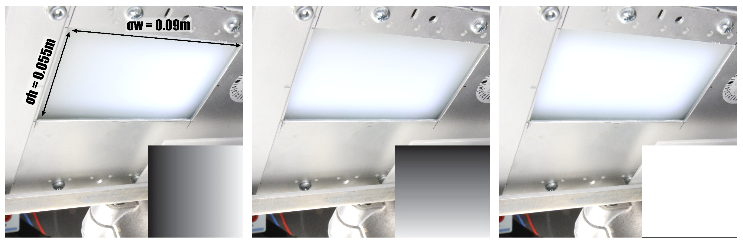
2.3. Deflectometry

To extract three-dimensional information from the surface of the rolling elements, the method presented in [27] is to be applied in a modified form. This method can be ideally adapted for use with a line scan camera by using a sufficiently fast exposure device. The illumination patterns presented in work [27] are used in a modified form. The formulas were adapted for the laboratory setup for rolling element testing. In this case, ${\sigma }_w$ stands for the screen width in meters, and ${\sigma }_h$ stands for the screen height in meters. The vector $\overrightarrow{\omega }$ describes the position on the screen. The intensity $P_{x/y}\left(\overrightarrow{\omega }\right)$ in the respective coordinate direction results as a linear brightness curve according to Formulas (1) and (2). Formula (3) was not adjusted and is adopted for this work.

$$P_x\left(\overrightarrow{\omega }\right)=\frac{1}{2}·(\frac{{\omega }_x}{{\sigma }_w}+1),$$

(1)

$$P_y\left(\overrightarrow{\omega }\right)=\frac{1}{2}·(\frac{{\omega }_y}{{\sigma }_h}+1),$$

(2)

$$P_c\left(\overrightarrow{\omega }\right)=1$$

(3)

According to Formula (1), a horizontal brightness gradient is created for $P_x$. This curve shows a linear brightness increase in the horizontal direction. Ideally, this goes from the brightness value of zero to the maximum possible brightness of the LEDs used. $P_y$ represented by Formula (2) is a vertical brightness curve that goes from the value 0 to the maximum possible brightness value of the LEDs. $P_y$ corresponds to $P_x$ rotated by 90°. $P_c$ described by Formula (3) is the full exposure of the object, which means that all LEDs are driven at full power. The resulting brightness gradients are generated by selectively controlling the brightness of the LEDs. The LEDs then illuminate a focusing screen that further homogenizes the pattern. In Figure 3, these brightness curves can be seen both on the real matrix and as a schematic.

The images recorded with the three illumination patterns, shown in Figure 3, contain the three images $L_x$, $L_y$, $L_c$. From these three images, the tilt information is extracted, as given in Formulas (4) and (5).

$$R_x=\frac{L_x}{L_c},$$

(4)

$$R_y=\frac{L_y}{L_c},$$

(5)

With the help of these two gradient images, the reflection vector $\overrightarrow{r}$ can now be calculated, according to Formula (6), for each pixel, considering the screen width ${\sigma }_w$, screen height ${\sigma }_h$, and the distance between the object and the screen d.

$$\overrightarrow{r}=\left[\begin{array}{c}\frac{{\sigma }_w}{\sqrt{{\sigma }_w^2+d^2}}·(2·R_x-1)\\ \frac{{\sigma }_h}{\sqrt{{\sigma }_h^2+d^2}}·(2·R_y-1)\\ \sqrt{1-{\overrightarrow{r_x}}^2-{\overrightarrow{r_y}}^2}\end{array}\right]$$

(6)

As the last step, the surface normal $\overrightarrow{n}$ is calculated pixel by pixel as the angle bisector between the reflection vector and the fixed camera vector $\overrightarrow{v}$, according to Formula (7).

$$\overrightarrow{n}=\frac{\overrightarrow{r}+\overrightarrow{v}}{\left||\overrightarrow{r}+\overrightarrow{v}\right||}$$

(7)

The result represents the gradient field of the surface and will be reconstructed as a virtual surface afterwards (cf. [27]).

2.4. Reconstruction

The reconstruction is the conversion of a vector field into a heightmap. The preceding deflectometric procedure directly provides the vector field serving as input. This field provides the surface slope in the X- and Y-direction in each pixel. Thus, an elevation map is to be created, which provides an height value for each pixel and thus virtually represents the surface. However, the following difficulties arise. If we see this conversion from gradient to height function as a simple integration of the values, it can be said that this is only possible for a real gradient field. By assuming that the input field is a gradient field, it is ensured that any integration path over the field yields the same heightmap. However, this is not guaranteed in the case of the field derived from the deflectometric method. The field recorded here cannot be considered a true gradient field due to noise and mismeasurements. Thus, different integration paths also yield different elevation map results. Another difficulty is boundary or starting values. In other words, a heightmap is a representation of a potential map. From the vector field, only the deviation to a fixed start value can be calculated. This start value must be defined in a meaningful way. Mostly, it is started at the value 0. After investigation of several reconstruction methods, it has been shown that two methods can provide good results. The first approach according to the work of Horn et al. [31] shows a detailed reconstruction of the surface. However, since this is an iterative approach, which in this application requires about 60,000 iterations to reconstruct a defect location, this approach has significant weaknesses in terms of computation time. Nevertheless, it will serve as a reference in this work due to the excellent reconstruction results. The second method following the approach of Yamaura et al. [34] provides a less detailed reconstruction of the surface. This approach relies on a reconstruction using a linear system of equations and on a description of the surface using B-spline functions. It can achieve fast reconstruction times. The realization and implementation of the two solutions followed the respective works [31,34].

3. Results

3.1. Image Acquisition and Deflectometry

The following system parameters result from the geometry and measurements performed:

• Resolution X-direction: $3.97$ $\mathsf{\mu }$$\mathrm{m}$ per pixel, at 4096 pixel per line
• Resolution Y-direction: $9.42$ $\mathsf{\mu }$$\mathrm{m}$ per pixel, at 3335 pixel per rotation

To be able to test the system practically, a rolling element was specifically deformed. For this purpose, the rolling element was clamped together with a metal ball in a vice with moderate force. The result is a hemispherical impression on the rolling element surface. This rolling element was recorded by the system and the defect location was cut out by software. The size of the cutout is $1.3$ $\mathrm{m}$$\mathrm{m}$ by $1.8$ $\mathrm{m}$$\mathrm{m}$. The following figure shows the results of the deflectometric process. First, the unprocessed image of the rolling element surface can be seen in Figure 4a. Next to this, in Figure 4b, the calculated gradient field is shown in the form of a normal map.

In the section of the defect location in Figure 4a, the image acquisition structure in the form of horizontal lines can be seen clearly. These lines are created by recording each line of the surface with three different illumination patterns. In addition, spatial brightness distribution can be seen in the form of shadows cast into the defect area. The question at this point is whether the shadowing leads to a loss of information in this area. After the deflectometric evaluation, which is shown in Figure 4b in the form of a normal map, the spherical shape of the defect can be seen easily. The areas around it have an almost flat surface. Only at the top of the defect can a bright edge be seen, which is probably due to shading, and thus to information loss at this point. Nevertheless, the deflectometric evaluation looks very promising.

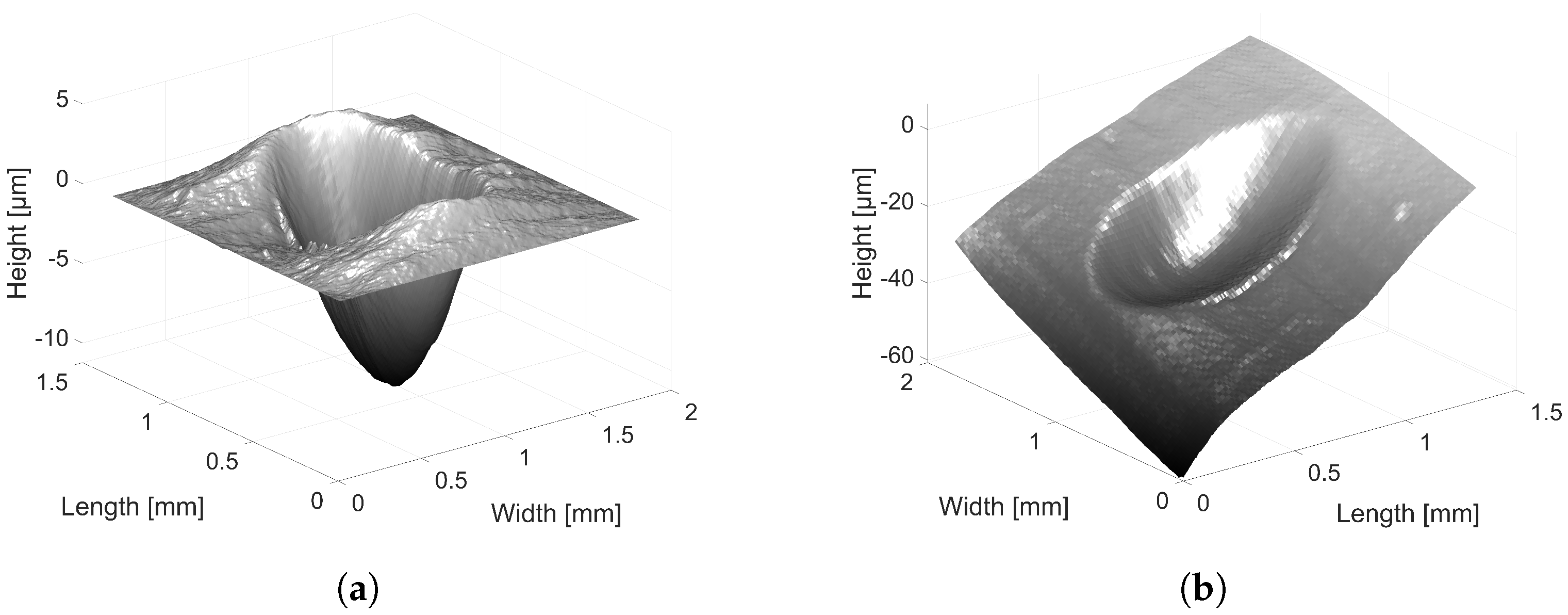
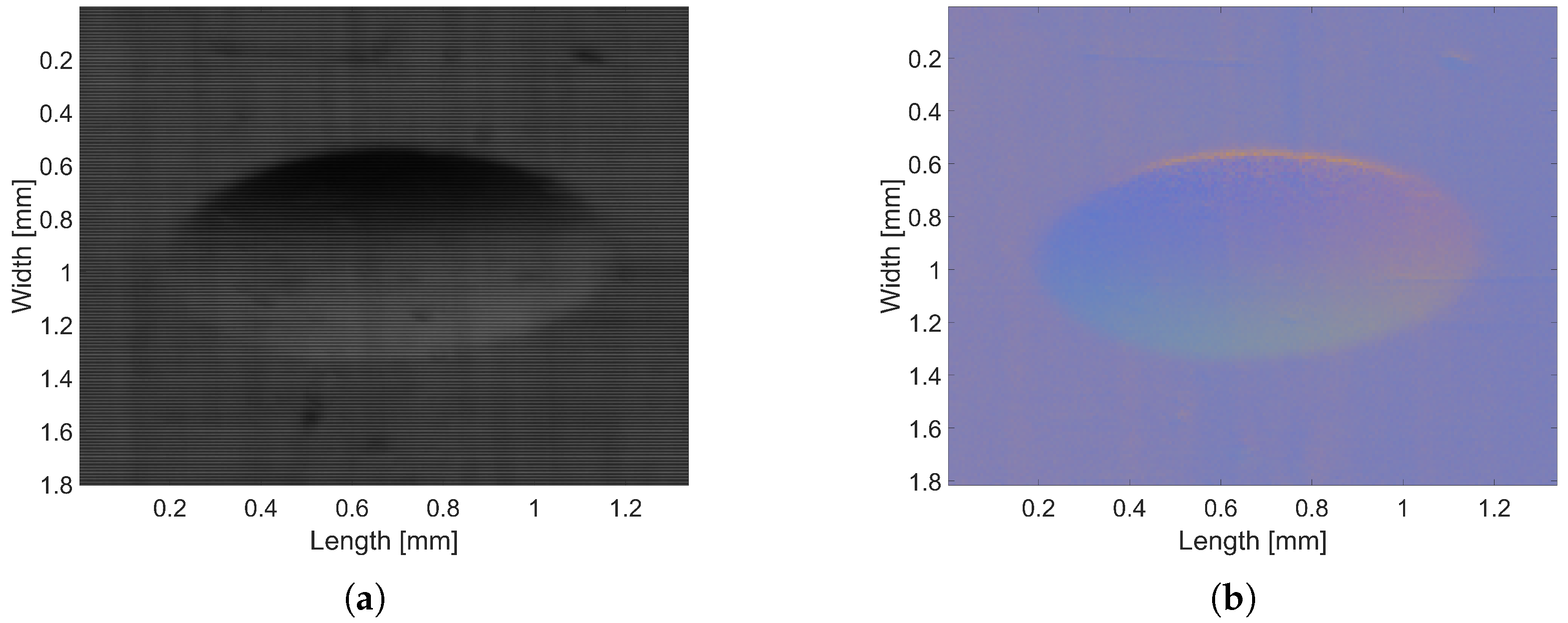
3.2. Reconstruction

The result of the deflectometric evaluation is then used to reconstruct the defect location. For this purpose, the two algorithms, presented in Section 2.4, by Horn et al. [31] and by Yamaura et al. [34] were used. The following Figure 5 shows a comparison of both algorithms.

It can be seen that the error location in Figure 5a is reconstructed in much more detail than in Figure 5b, this is due to the fact that in [34] the resolution of the height map is reduced by about half. In addition, in Figure 5b a systematic gradient can be seen in both the X- and Y-directions. This gradient could have been caused by an inaccuracy in the positioning of the light source, i.e., in the step of image acquisition. However, there are big differences between the two methods in terms of computing time, which will be considered in later sections.

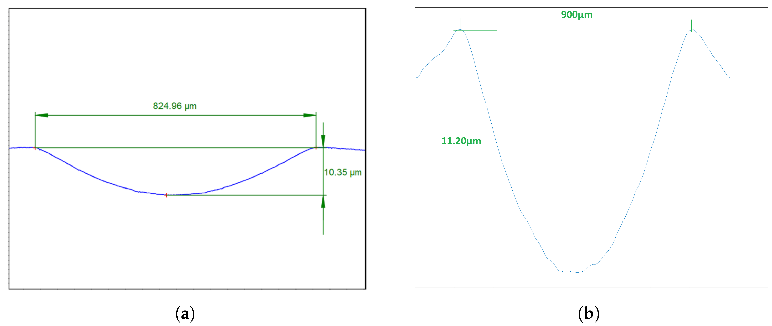
3.3. Reference Measurement

To evaluate the quality of the system, the defect was mechanically measured to a depth of $10.35$ $\mathsf{\mu }$$\mathrm{m}$. For comparison, the same rolling element was now optically recorded and reconstructed with approach [31]. The system measured the defect location to a depth of $11.20$ $\mathsf{\mu }$$\mathrm{m}$. The following Figure 6 shows a comparison of both measurements.

It can be seen that the two measurements have the same depth except for a small deviation. An evaluation of the height profile is difficult, because the mechanical measurement has a different pixel resolution, and therefore a different zoom level than the calculated solution. However, it can be said that, as expected, both methods describe a cross-section with an almost spherical shape.

3.4. Repeatability

To determine the repeatability of the measurement, 25 measurements of the rolling element described above were performed. For this purpose, the rolling element surface was recorded as described. Afterwards, an area of 1000 × 1000 pixels was cut out around the defect location. For this section, the gradient values were extracted and then reconstructed with approach [31]. The results in a 1000 × 1000 pixel elevation map that includes the fault location. To compare the measurements, the 100 deepest pixels for this measurement were determined. These were then used to calculate the mean and standard deviation for the depth of the defect location. The results are presented in the following

Table 1. Repeatability parameters.

Mean	m = −12.21 × 10−6 m
Standard deviation	σ = 1.7 × 10−7 m
Signal-to-noise ratio	71:1

.

3.5. Computing Time

For the system to be used as an inline inspection system, the parts should be inspected with sufficient speed. In this project, no optimization has yet been performed concerning computation time. The deflectometry and reconstruction calculations were performed using an Intel(R) Core(TM) i7-10510U processor on an HP ENVY ×360 (Model 15-dr1006ng) notebook. The following

Table 2. Computing times.

Recording of the mantle surface	5 $\mathbf{s}$
Deflectometric evaluation	1 $\mathrm{s}$
Reconstruction [31]	12 $\mathrm{s}$
Reconstruction [34]	2 $\mathrm{s}$
Best total time	8 $\mathrm{s}$

lists the acquisition and evaluation times for the defect.

4. Conclusions

The inspection system presented in this paper combines the use of a line scan camera with deflectometry techniques, allowing the extraction of three-dimensional surface information from cylindrical specular surfaces and subsequently reconstructing them with high accuracy. In addition, the reconstruction directly provides the absolute depth of defect locations. This additional information can then be evaluated depending on the specific application. The computing times of the system suggest that its use as an inline inspection system would be quite conceivable. It is possible to measure defects such as dents or scratches down to a depth of 15 $\mathsf{\mu }$$\mathrm{m}$. It is also possible to track surface deformations, which allows the system to be used for a wide range of problems. Comparing the system with existing inspection systems, it distinguishes itself by its high accuracy and reconstruction speed. There are significantly faster methods, such as eddy current inspection or two-dimensional optical inspection. However, these do not provide depth information on the surface. In terms of accuracy, better systems can be found in the literature, such as stylus methods or interferometric methods. However, due to the long acquisition times, these systems can only be used as inline systems to a limited extent. In addition, the presented system specializes in recording cylindrical reflective surfaces, which is not possible with methods such as PMD or FTP. Since the existing deflectometric methods are limited to the analysis of objects using a matrix camera and cannot accurately inspect the mantle surface of a cylindrical object [35], the presented system fills a gap in the literature by combining a deflectometric method with the use of a line scan camera. Thus, the system enables accurate and fast measurement of reflective cylindrical surfaces using deflectometric techniques. Even though the system gives promising results, this work should be seen only as an investigation of possibilities. Therefore, further validation of system-relevant parameters should take place in the future. For example, a correlation between screen size and angular resolution should be established. The maximum surface tilt at the system can provide valid information should also be investigated. In future studies, the illumination should be adjusted so that even very sharp-edged defect locations can be sufficiently illuminated. Here, it would be conceivable to set up the illumination spherically around the test object, as shown in [27]. To increase the application range of the system, a miniaturization of the component could be made to make the recording system as compact as possible. For the system to be used as an automatic inspection system, future work must develop a suitable evaluation of the data produced. Segmentation with the use of a two-dimensional image and subsequent three-dimensional evaluation of the defect locations found can be imagined here. In addition, the computation and evaluation times must be optimized. The aim should be to achieve an inspection time of around one second per part. It is uncertain if the system will be able to establish itself as an inspection system for rolling elements, since the benefit compared to two-dimensional inspection is not very high. Defects on a rolling element are unacceptable regardless, and therefore lead to exclusion of the defective part. However, an application in sleeve inspection or the production of linear guide rails, for example, would be conceivable.

References

- Ebayyeh, A.A.R.M.A.; Mousavi, A. A Review and Analysis of Automatic Optical Inspection and Quality Monitoring Methods in Electronics Industry. IEEE Access 2020, 8, 183192–183271. [Google Scholar] [CrossRef]
- Czimmermann, T.; Ciuti, G.; Milazzo, M.; Chiurazzi, M.; Roccella, S.; Oddo, C.M.; Dario, P. Visual-Based Defect Detection and Classification Approaches for Industrial Applications—A SURVEY. Sensors 2020, 20, 1459. [Google Scholar] [CrossRef] [PubMed] [Green Version]
- Pernkopf, F.; O’Leary, P. Image acquisition techniques for automatic visual inspection of metallic surfaces. NDT E Int. 2003, 36, 609–617. [Google Scholar] [CrossRef]
- Olver, A.V. The Mechanism of Rolling Contact Fatigue: An Update. Proc. Inst. Mech. Eng. Part J J. Eng. Tribol. 2005, 219, 313–330. [Google Scholar] [CrossRef]
- Yin, H.; Wu, Y.; Liu, D.; Zhang, P.; Zhang, G.; Fu, H. Rolling Contact Fatigue-Related Microstructural Alterations in Bearing Steels: A Brief Review. Metals 2022, 12, 910. [Google Scholar] [CrossRef]
- Singh, S.; Köpke, U.G.; Howard, C.Q.; Petersen, D. Analyses of contact forces and vibration response for a defective rolling element bearing using an explicit dynamics finite element model. J. Sound Vib. 2014, 333, 5356–5377. [Google Scholar] [CrossRef]
- Ashtekar, A.; Sadeghi, F.; Stacke, L.E. Surface defects effects on bearing dynamics. Proc. Inst. Mech. Eng. Part J J. Eng. Tribol. 2010, 224, 25–35. [Google Scholar] [CrossRef]
- Kaplan, K.; Kaya, Y.; Kuncan, M.; Minaz, M.R.; Ertunc, H.M. An improved feature extraction method using texture analysis with LBP for bearing fault diagnosis. Appl. Soft Comput. 2020, 87, 106019. [Google Scholar] [CrossRef]
- Kuncan, M. An Intelligent Approach for Bearing Fault Diagnosis: Combination of 1D-LBP and GRA. IEEE Access 2020, 8, 137517–137529. [Google Scholar] [CrossRef]
- Xu, Y.; Tian, W.; Zhang, K.; Ma, C. Application of an enhanced fast kurtogram based on empirical wavelet transform for bearing fault diagnosis. Meas. Sci. Technol. 2019, 30, 035001. [Google Scholar] [CrossRef]
- Prappacher, N.; Bullmann, M.; Bohn, G.; Deinzer, F.; Linke, A. Defect Detection on Rolling Element Surface Scans Using Neural Image Segmentation. Appl. Sci. 2020, 10, 3290. [Google Scholar] [CrossRef]
- Hatsukade, Y.; Okuno, S.; Mori, K.; Tanaka, S. Eddy-Current-Based SQUID-NDE for Detection of Surface Flaws on Copper Tubes. IEEE Trans. Appl. Supercond. 2007, 17, 780–783. [Google Scholar] [CrossRef]
- Tsukada, K.; Hayashi, M.; Nakamura, Y.; Sakai, K.; Kiwa, T. Small Eddy Current Testing Sensor Probe Using a Tunneling Magnetoresistance Sensor to Detect Cracks in Steel Structures. IEEE Trans. Magn. 2018, 54, 1–5. [Google Scholar] [CrossRef]
- Zhang, H.; Zhong, M.; Xie, F.; Cao, M. Application of a Saddle-Type Eddy Current Sensor in Steel Ball Surface-Defect Inspection. Sensors 2017, 17, 2814. [Google Scholar] [CrossRef] [Green Version]
- Bernieri, A.; Ferrigno, L.; Laracca, M.; Rasile, A.; Ricci, M. Ultrasonic non destructive testing on aluminium forged bars. In Proceedings of the 2017 IEEE International Workshop on Metrology for AeroSpace (MetroAeroSpace), Padua, Italy, 21–23 June 2017; pp. 223–227. [Google Scholar] [CrossRef]
- Kappes, W.; Bähr, W.; Schäfer, W.; Schwender, T.; Knam, A.; Knapp, F. Innovative solution for ultrasonic fabrication test of railroad wheels. In Proceedings of the 2014 IEEE Far East Forum on Nondestructive Evaluation/Testing, Chengdu, China, 20–23 June 2014; pp. 340–344. [Google Scholar] [CrossRef]
- Schmitz, V.; Barbian, O.A.; Gebhardt, W.; Salzburger, H.J. Moderne Verfahren der Ultraschallprüfung. Mater. Test. 1985, 27, 49–56. [Google Scholar] [CrossRef]
- Ren, C.; Xiu, X.Y.; Zhou, G.H. Research on Surface Defect Detection Technique of Rolling Element Based on Computer Vision. In Advanced Materials Research; Trans Tech Publications Ltd.: Bäch, Switzerland, 2014; Volume 1006, pp. 773–778. [Google Scholar] [CrossRef]
- Xian, W.; Zhang, Y.; Tu, Z.; Hall, E. Automatic visual inspection of the surface appearance defects of bearing roller. In Proceedings of the IEEE International Conference on Robotics and Automation, Cincinnati, OH, USA, 13–18 May 1990; Volume 3, pp. 1490–1494. [Google Scholar] [CrossRef]
- Hsu, C.Y.; Ho, B.S.; Kang, L.W.; Weng, M.F.; Lin, C.Y. Fast vision-based surface inspection of defects for steel billets. In Proceedings of the 2016 IEEE International Conference on Consumer Electronics-Asia (ICCE-Asia), Seoul, Korea, 26–28 October 2016; pp. 1–2. [Google Scholar] [CrossRef]
- Reindl, I.; O’Leary, P. Instrumentation and Measurement Method for the Inspection of peeled Steel Rods. In Proceedings of the 2007 IEEE Instrumentation Measurement Technology Conference IMTC 2007, Warsaw, Poland, 1–3 May 2007; pp. 1–6. [Google Scholar] [CrossRef]
- Xu, Y.; Gao, F.; Jiang, X. A brief review of the technological advancements of phase measuring deflectometry. PhotoniX 2020, 1, 14. [Google Scholar] [CrossRef]
- Zhang, Z.; Wang, Y.; Huang, S.; Liu, Y.; Chang, C.; Gao, F.; Jiang, X. Three-Dimensional Shape Measurements of Specular Objects Using Phase-Measuring Deflectometry. Sensors 2017, 17, 2835. [Google Scholar] [CrossRef] [Green Version]
- Su, X.; Chen, W. Fourier transform profilometry: A review. Opt. Lasers Eng. 2001, 35, 263–284. [Google Scholar] [CrossRef]
- Liu, Y.; Zhang, Q.; Zhang, H.; Wu, Z.; Chen, W. Improve Temporal Fourier Transform Profilometry for Complex Dynamic Three-Dimensional Shape Measurement. Sensors 2020, 20, 1808. [Google Scholar] [CrossRef] [Green Version]
- Chen, L.C.; Yeh, S.L.; Tapilouw, A.M.; Chang, J.C. 3-D surface profilometry using simultaneous phase-shifting interferometry. Opt. Commun. 2010, 283, 3376–3382. [Google Scholar] [CrossRef]
- Francken, Y.; Cuypers, T.; Bekaert, P. Mesostructure from specularity using gradient illumination. In Proceedings of the 5th ACM/IEEE International Workshop on Projector Camera Systems, Bali Way, CA, USA, 20 August 2008; p. 11. [Google Scholar] [CrossRef] [Green Version]
- Durou, J.D.; Aujol, J.F.; Courteille, F. Integrating the Normal Field of a Surface in the Presence of Discontinuities. In Proceedings of the International Workshop on Energy Minimization Methods in Computer Vision and Pattern Recognition, Bonn, Germany, 24–27 August 2009; Cremers, D., Boykov, Y., Blake, A., Schmidt, F.R., Eds.; Springer: Berlin/Heidelberg, Germany, 2009; pp. 261–273. [Google Scholar]
- Forsyth, D.A.; Ponce, J. Computer Vision—A Modern Approach, 2nd ed.; Pearson: London, UK, 2012; pp. 1–791. [Google Scholar]
- Frankot, R.; Chellappa, R. A method for enforcing integrability in shape from shading algorithms. IEEE Trans. Pattern Anal. Mach. Intell. 1988, 10, 439–451. [Google Scholar] [CrossRef] [Green Version]
- Horn, B.K.; Brooks, M.J. The variational approach to shape from shading. Comput. Vision Graph. Image Process. 1986, 33, 174–208. [Google Scholar] [CrossRef] [Green Version]
- Ng, H.S.; Wu, T.P.; Tang, C.K. Surface-from-Gradients without Discrete Integrability Enforcement: A Gaussian Kernel Approach. IEEE Trans. Pattern Anal. Mach. Intell. 2010, 32, 2085–2099. [Google Scholar] [CrossRef]
- Wei, T.; Klette, R. A Wavelet-Based Algorithm for Height from Gradients. In Proceedings of the International Workshop on Robot Vision, Auckland, New Zealand, 16–18 February 2001; Volume 1998, pp. 84–90. [Google Scholar] [CrossRef]
- Yamaura, Y.; Nanya, T.; Imoto, H.; Maekawa, T. Shape reconstruction from a normal map in terms of uniform bi-quadratic B-spline surfaces. Comput.-Aided Des. 2015, 63, 129–140. [Google Scholar] [CrossRef]
- Burke, J.; Pak, A.; Höfer, S.; Ziebarth, M.; Roschani, M.; Beyerer, J. Deflectometry for specular surfaces: An overview. arXiv 2022, arXiv:2204.11592. [Google Scholar]