Optimization and Diversification of Cryptocurrency Portfolios: A Composite Copula-Based Approach

Abstract

This paper focuses on the selection and optimisation of a cryptoasset portfolio, using the K-means clustering algorithm and GARCH C-Vine copula model combined with the differential evolution algorithm. This integrated approach allows the construction of a diversified portfolio of eight cryptocurrencies and determines an optimal allocation strategy making it possible to minimize the conditional value-at-risk of the portfolio and maximise the return. Our results show that stablecoins such as True-USD are negatively correlated to the other cryptoassets in the portfolio and could therefore be a safe haven for crypto-investors during market turmoil. Our findings are in line with previous studies exhibiting stablecoins as potential diversifiers.

1. Introduction

In the modern theory of portfolio selection, investor preferences are defined in terms of profit and risk. The return of a portfolio is a combination of the returns of the weighted assets that compose it. The risk of a portfolio is a function of the correlation between the assets that compose it. It is therefore important to diversify your portfolio so as not to suffer from large fluctuations in the asset prices due to the reoccurrence of shocks in the financial sphere and the increase in geopolitical and macroeconomic uncertainties. These fluctuations in assets prices are also linked to the general health of the sector in which one invests. It is well known that, for example, the technology, telecommunications and cryptocurrency markets are marked by strong fluctuations. Diversification therefore obeys the famous adage in portfolio management which says: “you must not put all your eggs in one basket”. Thus, according to the modern portfolio theory developed by Markowitz [1], the ultimate goal of portfolio managers is to combine a set of assets with maximum profit for a given level of risk or alternatively, with minimum risk for a given level of profit. This is the efficient portfolio.

Indeed, the frantic search for diversification and the creation in 2009 of new digital financial assets based on the highly secure “distributed ledger technology” (DLT) and cryptography, have led portfolio managers and many financial institutions to successfully integrate this new class of crypto-assets into the financial world. Cryptocurrencies or virtual currencies (VC) are the main components of crypto-assets defined as a type of unregulated or decentralised digital currency, created and generally controlled by its developers, used and accepted by members of a virtual community. Therefore, it is easy to become a cryptocurrency market player as long as one has some basic knowledge about their functionality. VCs have many unusual characteristics compared to other financial instruments such as lack of centralised control, (pseudo-) anonymity, difficulties of estimating their value, their hybrid characteristics combining aspects of traditional financial instruments with those of intangible assets, and the rapid evolution of technology which underpins them. Those erratic characteristics have contributed to their popularity and the rapid growth of their total market capitalisation which was estimated to 2.37 trillion US dollars in May 2021 (https://coinmarketcap.com/all/views/all/, accessed on 20 May 2021) with Bitcoin, the oldest and most traded and valuable cryptocurrency representing 44% and other altcoins (alternative coin to Bitcoin) share the rest. The abovementioned facts and the potential shown by cryptocurrency to become a cheap alternative to conventional currencies can justify the interests of investors, portfolio managers, financial institutions and researchers on the opportunities offered by the cryptocurrencies markets.

A good portfolio is one that gives a maximum return for a given level of risk or one that gives the minimum risk for a given level of return. Thus, a good portfolio must combine different assets satisfying a set of given restriction in order to achieve that goal. Hence, this situation requires mathematical modelling for portfolio selection and optimization. In practice, the portfolio selection (or allocation) and optimisation problems must take into account real characteristics of the assets that compose it, such as correlation and dependencies that may exist between assets, market risks, quantity constraint which imposes a limit on the number of assets in the portfolio, weigh allocation constraints limiting the proportion of each asset in the portfolio and transaction cost. This leads to a complex optimization problem.

Markowitz’s model [2] was the first to formalise an analytical response to the asset allocation and selection problem. Indeed, Markowitz considers the particular case of investors with risk preferences adjusting to quadratic utility functions. The analytical solution to this problem gives all the portfolios that form the “so-called efficient frontier”, which represents the optimal returns to be achieved for each level of risk. In order to overcome the shortcomings of the Markowitz approach, alternative approaches have been developed. Bares et al. [3] discuss portfolio optimization within the framework of the expected utility approach using iso-elastic utility functions. Javed et al. [4], Khan et al. [5] as well as Jurczenko et al. [6] proposed the analysis based on moments of higher orders. Hunjra et al. [7], Krokhmal et al. [8] as well as Agrawal and Naik [9] construct optimal portfolios using alternative risk measures. All these methods have shown their performance compared to the results given through classical analysis. This confirms the interest in dealing with issue of portfolio selection outside the Gaussian framework.

One of the approaches aimed at relaxing the Gaussian framework imposed by the mean-variance approach concerns the modelling of the asymmetric nature of the dependency structure of the portfolio [10]. One of the solutions is that of copula functions, vine copula specification based on sequential method (also based on maximum spanning tree algorithm and maximum likelihood estimation of the pair-copula parameters) used to solve the joint probability modelling problem. The use of copula functions in the context of the asset allocation problem is still relevant today. Mba et al. [11], use GARCH-differential evolution t-copula method in order to optimize and analyse cryptocurrency portfolio risk and return within the framework of a multi-period setting type approach. More recently, Boako et al. [12] integrated copula functions into a GARCH modelling to analyse the structural interdependencies among seventeen cryptocurrency prices and to optimise the portfolio Value-at-Risk (VaR). In the same wake Mba and Mwambi [13] used a two state Markov-switching technique combined with R-vine copula and GARCH (MSCOGARCH) to model heavy tail dependencies and structural breaks within the states of Markov switching with the aim of achieving a maximum return with a minimum conditional value-at-risk of a portfolio of top ten virtual currencies (in term of market capitalisation).

The results obtained in the aforementioned works on the selection, allocation and optimization of crypto-asset portfolios present some shortcomings, namely:

• These portfolios have a very low VaR or Conditional VaR and high return (above 50%) which is not in line with the crypto-market dynamics which is unregulated, highly volatile and permanently subjected to extreme events.
• In addition, these portfolios are only made up of the best performing crypto assets, which are strongly and positively correlated between themselves and in particular with Bitcoin and, therefore, cannot constitute a diversified portfolio.

The fundamental objective of this paper is to improve the work of Mba [11,13] and Boako et al. [12] on the optimization and selection of cryptocurrency portfolios in order to address the aforementioned shortcomings. The issue of non diversification is addressed by applying a machine learning technique known as K-means algorithm, reinforce with hierarchical clustering which groups similar assets into a cluster exhibiting a certain level of dissimilarity with other clusters. In fact, the technique will be applied to the top hundred cryptocurrencies consisting of different class of cryptoassets such as: coins, token, stablecoins, decentralised finance token (DeFi) and non fungible token (NFT). To overcome the issue of underestimation of the risk and overestimation of the returns, we preprocess the input data for the optimisation of CVaR and expected returns as follows: inverse transformation of the copula output using the quantile of the skew student-t distribution which constitutes the marginal in the copula fitting.

The novelty of our integrated approach is the combination of the machine learning technique (clustering and hierarchical algorithm), econometric model (GJR-GARCH), differential evolution algorithm and vine copula model in the selection and optimisation of a cryptoasset portfolio. Our results highlight the fact that, the top ten or twenty cryptocurrencies cannot constitute a diversify portfolio since they are highly and positively correlated. Another take away of our findings is that stablecoin such as True-USD is negatively correlated to the other cryptoassets in the portfolio and could therefore be safe haven for crypto-investors when market experiences extreme events.

The roadmap of the contributions of this work is organised as follows. First, in Section 2, a non-exhaustive literature review on the application of copula in the portfolio optimisatio is presented; a survey of different risk measures that can be useful in cryptocurrency portfolio optimization problems is also discussed. Section 3 is devoted to the methodology that was used to achieve the objective of this paper. In Section 4, we implement the methodology and present the empirical results. In the last section, we summarise the main results obtained in the previous section and we will also point out their weaknesses and strengths.

2. Methodology

This section presents the theoretical framework of the paper. We introduce the objective and the methods used to present our results.

2.1. Machine Learning: K-Means Clustering

Definition 1.

K-means is an unsupervised algorithm for non-hierarchical clustering. It allows the observations of the data set to be grouped into distinct clusters. Thus, similar data will be found in the same cluster. In addition, an observation can only be found in one cluster at a time (membership exclusivity). The same observation cannot therefore belong to two different clusters.

K-means is an iterative algorithm that minimizes the sum of the distances between each observation and the centroid. The initial choice of number K of the centroids determines the final result. Admitting a cloud of a set of points (data or observations), K-means changes the points of each cluster until the sum can no longer decrease. The result is a set of compact and clearly separated clusters, provided the researcher chooses the right K value for the number of clusters.

The convergence of the K-means Algorithm 1 can be one of the following conditions:

• A pre-set number of iterations, in this case K-means will perform the iterations and stop regardless of the shape of compound clusters.
• Stabilization of cluster centers (centroids no longer move or change during iterations).

Algorithm 1: K-means Algorithm

Input: K the number of clusters to be formed X the Training Set ($m\times n$ data matrix) Output: Randomly choose $K<m$ points (K rows of the data matrix). These points are the centers of the clusters (called centroid). Assign a cluster to each point (or observation), randomly. Calculate the centroid of each cluster (i.e. the vector of the means of the different variables) For each point calculate its Euclidean distance with the centroids of each of the clusters Assign the closest cluster to the object Calculate the sum of the intra-cluster variability Repeat steps 3 to 5, until an equilibrium is reached, that is convergence: no more change in clusters, or stabilization of the sum of the intra-cluster variability.

2.2. Vine-Copula

This subsection describes the characteristics necessary for a function to be a copula, as well as some of their properties. Before mentioning them, some preliminary definitions and results are useful. In fact, here is the idea behind the copula approach.

Let $X=(X_1,\dots ,X_n)$ be a vector of n random variables for which we want to construct the joint distribution function. Let assume that, $X_1,\dots ,X_n$ are random variables with the following marginal distributions $F_1,\dots ,F_n$, such as $F_i\left(x_i\right)=P(X_i\le x_i)=u_i$ (the probability that the measure of $X_i$ be less than $x_i$). Then the joint distribution function is given by

$$F(x_1,\dots ,x_n)=P(X_1\le x_1,\dots ,X_n\le x_n).$$

(1)

Definition 2.

An n dimensional ($n\ge 2$) copula is a function $C:I^n⟶I$ satisfying the following properties:

1.

C is non-decreasing that is $C(0,\dots ,x_i,\dots ,0)=0,$ for all $x_i\in I=[0,1]$

2.

C possess one dimensional uniform margins on $C_i$, that is:

$C_i\left(x_i\right)=C(1,\dots ,1,x_i,1,\dots ,1)=x_i$ for all $x_i\in I$. $C_i$ is an invariant non-decreasing transformation of the marginal.

We can now show the link between copulae and random variables. Copulas are of interest in statistics thanks to the theorem proposed by Sklar [14].

Theorem 1.

Assume $F=(F_1,\dots ,F_n)$ is an n dimensional joint distribution function with marginal distribution function $F_i(i=1,\dots ,n)$. Then, there exists a copula C such that for all $\mathit{x}=(x_1,\dots ,x_n)\in I^n$

$$F\left(\mathit{x}\right)=C(F_1\left(x_1\right),\dots ,F_n\left(x_n\right))$$

If $F_1,\dots ,F_n$ are continue, then C is unique. Otherwise C is non-unique on $I^n$.

In addition, if $F_1,\dots ,F_n$ are distribution function on I and if C is a copula, then the function $F\left(\mathit{x}\right)=C(F_1\left(x_1\right),\dots ,F_n\left(x_n\right))$ is a joint distribution function on $I^n$.

The canonical representation of the copula density function is given as

$$c(u_1,\dots ,u_n)=\frac{{\partial }^{n}C(u_1,\dots ,u_n)}{\partial u_1,\dots ,\partial u_n}$$

(2)

To obtain the density of the n-dimension distribution F, the following relation is used

$$f(x_1,\dots ,x_n)=c(F_1\left(x_1\right),\dots ,F_n\left(x_n\right))\prod _{i=1}^n{f}_i\left(x_i\right)$$

(3)

where $f_i$ is the density of the marginal distribution $F_i$.

Copula functions constitute an advantageous statistical tool for constructing and simulating multivariate distributions. The literature devoted to the copula approach provides us with different types of density functions which can be summarized in two categories of families: the family of elliptical copulas and that of Archimedean copulas.

Table 1. Copula component.

No.	Elliptical Distribution	Parameter Range	Kendall’s $\mathit{\tau }$	Tail Dependence
1	Gaussian	$\rho \in (-1,1)$	$\frac{2}{\pi }arctan\left(\rho \right)$	0
2	Student-t	$\rho \in (-1,1),\nu >2$	$\frac{2}{\pi }arctan\left(\rho \right)$	$2t_{\nu +1}(-\sqrt{\nu +1}\sqrt{\frac{1-\rho }{1+\rho }})$
No.	Name	Generator Function	Parameter Range	Kendall’s$\mathbf{\tau }$	Tail Dependence
					(Lower, Upper)
3	Clayton	$\frac{1}{\theta }(t^{-\theta }-1)$	$\theta >0$	$\frac{\theta }{\theta +2}$	$(2^{-1/\theta },0)$
4	Gumbel	${(-logt)}^{\theta }$	$\theta \ge 1$	$1-\frac{1}{\theta }$	$(0,2-2^{1/\theta })$
5	Frank	$-log\left[\frac{e^{-\theta t}-1}{e^{-\theta }-1}\right]$	$\theta \in \mathbb{R}/0$	$1-\frac{4}{\theta }+4\frac{D_1\left(\theta \right)}{\theta }$	$(0,0)$
6	Joe	$-log[1-{(1-t)}^{\theta }]$	$\theta >1$	$1+\frac{4}{{\theta }^2}{\int }_0^{1}log\left(t\right){(1-t)}^{\frac{\theta (1-\theta )}{\theta }dt}$	$(0,2-2^{1/\theta })$
7	BB1	${(t^{-\theta }-1)}^{\theta }$	$\theta >0,\delta \le 1$	$1-\frac{2}{2(\theta +2)}$	$(2^{-1/\theta \delta },2-2^{1/\theta })$
8	BB6	${(-log[1-{(1-t)}^{\theta }])}^{\theta }$	$\theta >0,\delta \le 1$	$1+4{\int }_0^1(-log(-1{(1-t)}^{\theta }+1))$	$(0,2-2^{1/\theta \delta })$
				$\times \frac{(1-t-{(1-t)}^{-\theta }+t{(1-t)}^{-\theta })}{\theta \delta }dt$
9	BB7	${[1-{(1-t)}^{\theta }]}^{-\delta }-1$	$\theta \ge 1,\delta >0$	$1-\frac{2}{\theta (2-\theta )}+\frac{4}{{\theta }^{2\delta }}B(\frac{2-\theta }{\theta },\delta +2)$	$(2^{-1/\theta },2-2^{1/\theta })$
10	BB8	$-log\left[\frac{1-{(1-\theta t)}^{\theta }}{1-{(1-\theta )}^{\theta }}\right]$	$\theta \ge 1,\delta \le 1$	$1+4{\int }_0^1(-log\left(\frac{{(1-t\delta )}^{\theta }-1}{{(1-\delta )}^{\theta }-1}\right)$	$(0,0)$
				$\times \frac{1-1\delta -{(1-t\delta )}^{-\theta }+t\delta {(1-t\delta )}^{-\theta }}{\theta t}dt$

and

Table 2. Popular Archimedean copulas functions.

Name	Bivariate Copula ${\mathit{C}}_{\mathit{\theta }}(\mathit{x},\mathit{y})$	Parameter Range
Clayton	${\left[\max \{x^{-\theta }+y^{-\theta }-1;0\}\right]}^{-1/\theta }$	$\theta \in \left[-1,\infty \right.)-\left\{0\right\}$
Gumbel	$exp[-{\left({(-logx)}^{\theta }+{(-logy)}^{\theta }\right)}^{1/\theta }]$	$\theta \in \left[1,\infty \right.)$
Frank	$-\frac{1}{\theta }log\left[1+{\displaystyle \frac{(exp(-\theta x)-1)(exp(-\theta y)-1)}{exp(-\theta )-1}}\right]$	$\theta \in \mathbb{R}-\left\{0\right\}$
Joe	$1-{\left[{(1-x)}^{\theta }+{(1-y)}^{\theta }-{(1-x)}^{\theta }{(1-y)}^{\theta }\right]}^{1/\theta }$	$\theta \in \left[1,\infty \right.)$
Independent	$xy$

show different properties of popular copulas functions.

In practical applications, modelling using copula with a large set of high-dimensional variables, such as in this paper (a set of eight cryptocurrencies), has some limitations. These limitations can be parameters restriction and the selection of the appropriate copula function. Joe [15] proposed an alternative which is the use of vine-copulas method for high-dimensional data. 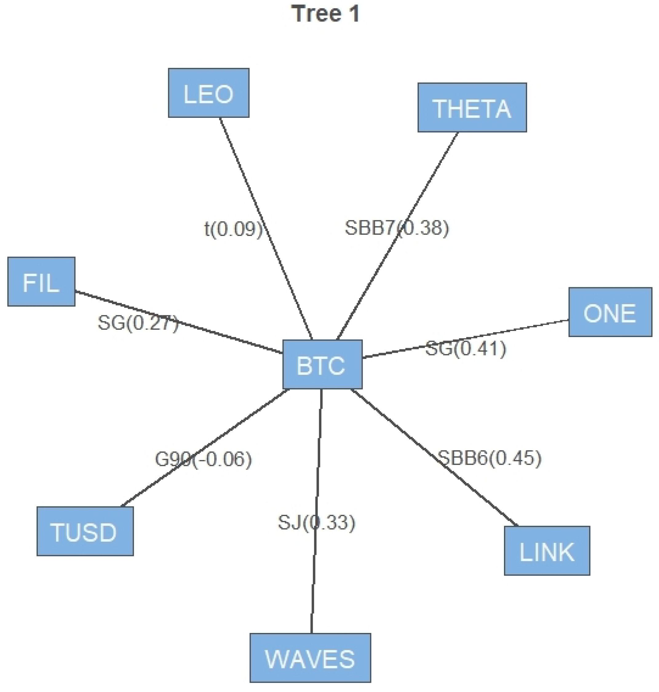Thus vine copulas, described by Bedford and Cooke [16,17] are flexible graphical models to describe multivariate copulas constructed using a cascade of bivariate copulas or pair-copulas. In this paper we will use C (canonical) and R (regular) vine copula specification.

2.3. GARCH-Copula Differential Evolution (DE): (GJR-GARCH-DE-C-Vine-Copula)

In many works, the copula approach is directly applied to returns of financial assets. Nevertheless, we recognize the stylised facts related to the fat tail distributions and the phenomenon of volatility clustering observed in financial time series data. Given this fact, it is useful to introduce GARCH models in order to filter these distributions. Then, the copula model can be used to model the dependency structure between the standardised innovations considered here as iid observations.

Here, we opt for GJR-GARCH(1,1) because it accounts for the leverage effect that creates asymmetry in the dynamics of the variance of the financial returns. More details on this model can be found in the works of Glosten et al. [18]. We recall that if a n-dimensional vector of time series variables (returns) $x_t=(x_{1,t},,x_{2,t},\dots ,x_{n,t})$ is assumed to follow a GARCH-Copula modelling type, by construction the joint distribution function is given in the following form

$$F\left({\mathit{x}}_t\right|{\mathit{\mu }}_t,{\mathit{\sigma }}_t)=C\left(F_1\left(x_{1,t}\right|{\mu }_{1,t},{\sigma }_{1,t}),\dots ,F_n\left(x_{n,t}\right|{\mu }_{n,t},{\sigma }_{n,t})\right)$$

where C is the n-dimensional copula, $F_i$ are the conditional marginal distribution functions relative to $x_{i,t}$, whose dynamics are described by the intercept ${\mu }_{i,t}$ which corresponds to the conditional mean and by an error term ${ϵ}_{i,t}=\sqrt{{\sigma }_{i,t}}{\nu }_{i,t}$, which can be constant or time dependent as in a GJR-GARCH(1,1) specification

$$\begin{array}{cc}\hfill x_{it}& ={\mu }_{i,t}+{ϵ}_{i,t}\hfill \\ \hfill {ϵ}_{i,t}& =\sqrt{{\sigma }_{i,t}}{\nu }_{i,t}\hfill \\ \hfill {\sigma }_t^2& ={\alpha }_0+{\beta }_1{\sigma }_{t-1}^2+({\alpha }_1+{\gamma }_1{\mathbb{I}}_{{ϵ}_{t-1}<0}){ϵ}_{t-1}^2\hfill \end{array}$$

(4)

where ${\sigma }_{i,t}$ is the conditional variance of the series $x_{i,t}$, given the prior information to time t, and ${\nu }_{i,t}=\frac{{ϵ}_{i,t}}{\sqrt{{\sigma }_{i,t}}}$ are iid random variables characterising the standardised innovation, considered as white noise with zero mean and variance equals 1 (${\nu }_t\sim N(0,1)$). ${\mathbb{I}}_{{ϵ}_{t-1}<0}=1$ if ${ϵ}_{t-1}<0$, otherwise ${\mathbb{I}}_{{ϵ}_{t-1}<0}=0$ and ${\gamma }_1{\mathbb{I}}_{{ϵ}_{t-1}<0}{ϵ}_{t-1}^2$ is the term related to the leverage effect.

The differential evolution initiated by Storn and Price [19] is a nonlinear optimization algorithm that has been extremely successful since its conception and was originally created to solve continuous problems. The algorithm is inspired from evolutionary biology operations which follow the following steps: initialisation, mutation, recombination and selection on a given population to minimise an objective function through successive generations. The algorithm uses alteration and selection operator to transform progressively a population of candidate solution.

Consider a population $\omega =({\omega }_1,\dots ,{\omega }_n)$ of size n and the objective function $h({\omega }_1,{\omega }_2,\dots ,{\omega }_n)$ to be optimised. The optimisation process is as follows [20,21]:

• Initial population
  The initial generation is created randomly, either by the computer or the user.
  Given the population ${\omega }_{ki}^g=({\omega }_{k1}^g,{\omega }_{k2}^g,\dots ,{\omega }_{kn}^g)$, where the number g represents the generation order and $k=1,2,\dots ,N$. The initial population or first generation is created as

  $${\omega }_{ki}={\omega }_{ki}^L+rand\left(\right)({\omega }_{ki}^U+{\omega }_{ki}^L)$$

  where ${\omega }_{ki}^L$ and ${\omega }_{ki}^U$ are lower and upper bounds of $\omega$ respectively, $rand\left(\right)$ a randomly generated number and $i=1,2,\dots ,n$.
• Mutation
  The evolutionary process of a generation follows a simple cycle, making it possible to sequentially improve each of the N individuals. Thus, each of the N individuals is called upon to be the target vector in turn. An initial mutant vector ${\mathit{u}}_k^{g+1}$ is created using a mutation process which simply involves adding the weighted difference of two other individuals randomly selected in the population to a third party vector as demonstrated by Equation (5).

  $${\mathit{u}}_k^{g+1}={\omega }_{jk}^g+c_1({\omega }_{lk}^g-{\omega }_{sk}^g),j\ne l\ne s.$$

  (5)

  where $k=1,2,\dots ,N.$ In Equation (5), the coefficient $c_1$ is the mutation coefficient which can be adjusted to control the amplitude of the mutations.
• Recombination
  Let us assume that each individual of the population will become a target vector. Assuming ${\omega }_{ki}^g$ is the target vector a discrete recombination process then creates a new or trial vector ${\mathit{v}}_{ki}^{g+1}$ by crossing the newly created mutant vector ${\mathit{u}}_k^{g+1}$ to the target vector.

  $${\mathit{v}}_{ki}^{g+1}=\left\{\begin{array}{c}{\mathit{u}}_{ki}^{g+1},\mathrm{if}rand\left(\right)\le C_p\mathrm{or}i=I_{rand}i=1,2,\dots ,n;\hfill \\ {\omega }_{ki}^g,d\mathrm{if}rand\left(\right)>C_p\mathrm{or}i\ne I_{rand}k=1,2,\dots ,N\hfill \end{array}\right.$$

  where $I_{rand}$ is an integer, randomly selected in $[1,n]$ and the recombination probability $C_p$ makes it possible to manage the level of involvement of both the target and mutant vector in the creation of the new vector.
• Selection

  $${\omega }_{ki}^{g+1}=\left\{\begin{array}{c}{\mathit{v}}_{ki}^{g+1},\mathrm{if}h\left({\mathit{v}}_{ki}^{g+1}\right)<h\left({\omega }_{ki}^g\right)\hfill \\ {\omega }_{ki}^g,\mathrm{otherwise}.\hfill \end{array}\right.$$

  (6)
  The condition in Equation (6), helps to avoid creating clones by ensuring that the new vector or solution has at least a dimension resulting from the mutant vector. Then, a selection will allow one to choose the best of the two solutions between ${\mathit{v}}_{ki}^{g+1}$ and ${\omega }_{ki}^g$. By observing the stages of mutation and recombination well it is obvious that to be functional, the number of individuals in the population must be at least 4.

2.4. Efficient Portfolio and Optimisation

An efficient portfolio is a portfolio whose expected return ${\mu }_p$ is maximum for a given level of risk, or whose risk is minimal for a given return. Efficient portfolios are on the “efficient frontier” of the set of portfolios in the plane $({\sigma }_p^2,{\mu }_p)$. The first question an investor asks himself is obviously to know: Which efficient portfolio offers the lowest level of risk? Our aim, therefore, is to determine this efficient frontier or at least to find a function which allows to determine the optimal portfolio for a target level of return ${\mu }_p$. This problem can be formulated as below:

$$\left\{\begin{array}{c}\min \left({\mathit{\omega }}^T\mathit{\sigma }\mathit{\omega }\right)\hfill \\ \mathrm{subject\; to}\hfill \\ {\mathit{\omega }}^{T}E\left(R_p\right)={\mu }_p\hfill \\ {\mathit{\omega }}^T\mathbf{1}=1\hfill \end{array}\right.$$

(7)

where $\mathbf{1}$ is a n vector column of 1.

In this paper, we chose the conditional value at risk (CVaR) as risk measure and follow Rockafellar and Uryasev [22] optimisation approach for problem (7).

Let $l(\mathit{\omega },\mathbf{R}):{\mathbb{R}}^n\times {\mathbb{R}}^n\to \mathbb{R}$ denote a loss function characterise par the decision (weight) vector $\mathit{\omega }$ and the return (random) vector R. The probability that the loss function $l(\mathit{\omega },\mathbf{R})$ never exceeds the threshold $\alpha \in (0,1)$ is given by

$$\begin{array}{cc}\hfill F\left[l\right(\mathit{\omega },\mathbf{R}),\alpha ]& =P\left\{l\right(\mathit{\omega },\mathbf{R})\le \alpha \}\hfill \\ \hfill & :={\int }_{l(\mathit{\omega },\mathbf{R})\le \alpha }P\left(\mathbf{R}\right)d\mathbf{R}\hfill \end{array}$$

and the value at risk for a certain level of confidence $\beta \in (0,1)$, is given by:

$$Va{R}_{\beta }\left[l(\mathit{\omega },\mathbf{R})\right]:=\inf \{\mathbf{R}\in {\mathbb{R}}^n:F[l(\mathit{\omega },\mathbf{R}),\alpha ]\ge \beta \},$$

and the formula of the conditional value at risk by

$$\begin{array}{cc}\hfill CVa{R}_{\beta }\left[l(\mathit{\omega },\mathbf{R})\right]& =E\left[l(\mathit{\omega },\mathbf{R})|l(\mathit{\omega },\mathbf{R})\ge Va{R}_{\beta }\left[l(\mathit{\omega },\mathbf{R})\right]\right]\hfill \\ \hfill & :=\frac{1}{1-\beta }{\int }_{l(\mathit{\omega },\mathbf{R})\ge Va{R}_{\beta }\left[l(\mathit{\omega },\mathbf{R})\right]}l(\mathit{\omega },\mathbf{R})P\left(\mathbf{R}\right)d\mathbf{R}\hfill \end{array}$$

Since it depends by construction on the function $Va{R}_{\beta }\left[l(\mathit{\omega },\mathbf{R})\right]$ which itself depends on $\mathit{\omega }$, the optimization of CVaR can sometimes be difficult to approach. Without having recourse to an analytical representation of VaR, Rockafellar and Uryasev [22] formulate the following auxiliary function

$$F[l(\mathit{\omega },\mathbf{R}),\alpha ]:=\alpha +\frac{1}{1-\beta }E\left[max\left\{l(\mathit{\omega },\mathbf{R})-\alpha ,0\right\}\right]$$

(8)

and demonstrate that

$$CVa{R}_{\beta }\left[l(\mathit{\omega },\mathbf{R})\right]=\underset{\alpha \in \mathbb{R}}{\inf }F[l(\mathit{\omega },\mathbf{R}),\alpha ]$$

(9)

The advantage of using the auxiliary function $F\left[l\right(\mathit{\omega },\mathbf{R}),\alpha ]$ is twofold: Firstly it is jointly convex with respect to $\alpha$ and $\mathit{\omega }$, provided that the loss function $l(\mathit{\omega },\mathbf{R})$ is also convex with respect to $\mathit{\omega }$. Secondly we do not have to choose a value for $\alpha$ beforehand, which can be difficult in practice. This is naturally derived during the optimization process based on the chosen confidence level.

Rockafellar and Uryasev [22] finally show that minimizing $CVa{R}_{\beta }\left[l(\mathit{\omega },\mathbf{R})\right]$ with respect to $\omega$ is equivalent to minimizing $F\left[l\right(\mathit{\omega },\mathbf{R}),\alpha ]$ with respect to $(\mathit{\omega },\alpha )\in {\mathbb{R}}^n\times (0,1)$, that is

$$\underset{\mathit{\omega }\in \mathbb{R}}{\min }CVa{R}_{\beta }\left[l(\mathit{\omega },\mathbf{R})\right]=\underset{(\mathit{\omega },\alpha )\in {\mathbb{R}}^n\times (0,1)}{\min }F[l(\mathit{\omega },\mathbf{R}),\alpha ]$$

(10)

Since ${\mathbb{R}}^n$ is convex by definition, (10) is therefore a convex optimization problem.

The optimal value of the conditional value at risk optimization problem (10) of a crypto-asset portfolio, can be found by solving the following convex optimization problem:

$$\underset{(\mathit{\omega },\alpha )\in {\mathbb{R}}^n\times (0,1)}{\min }F[l(\mathit{\omega },\mathbf{R}),\alpha ]$$

(11)

subject to

$$\left\{\begin{array}{c}{\mathit{\omega }}^{T}E\left(R_p\right)={\mu }_p\hfill \\ {\mathit{\omega }}^T\mathbf{1}=1\hfill \\ {\omega }_i\ge 0,1,\dots ,n.\hfill \end{array}\right.$$

(12)

2.5. Snapshot of the Methodology

The nine steps below are followed for the analysis on the CVaR:

step 1

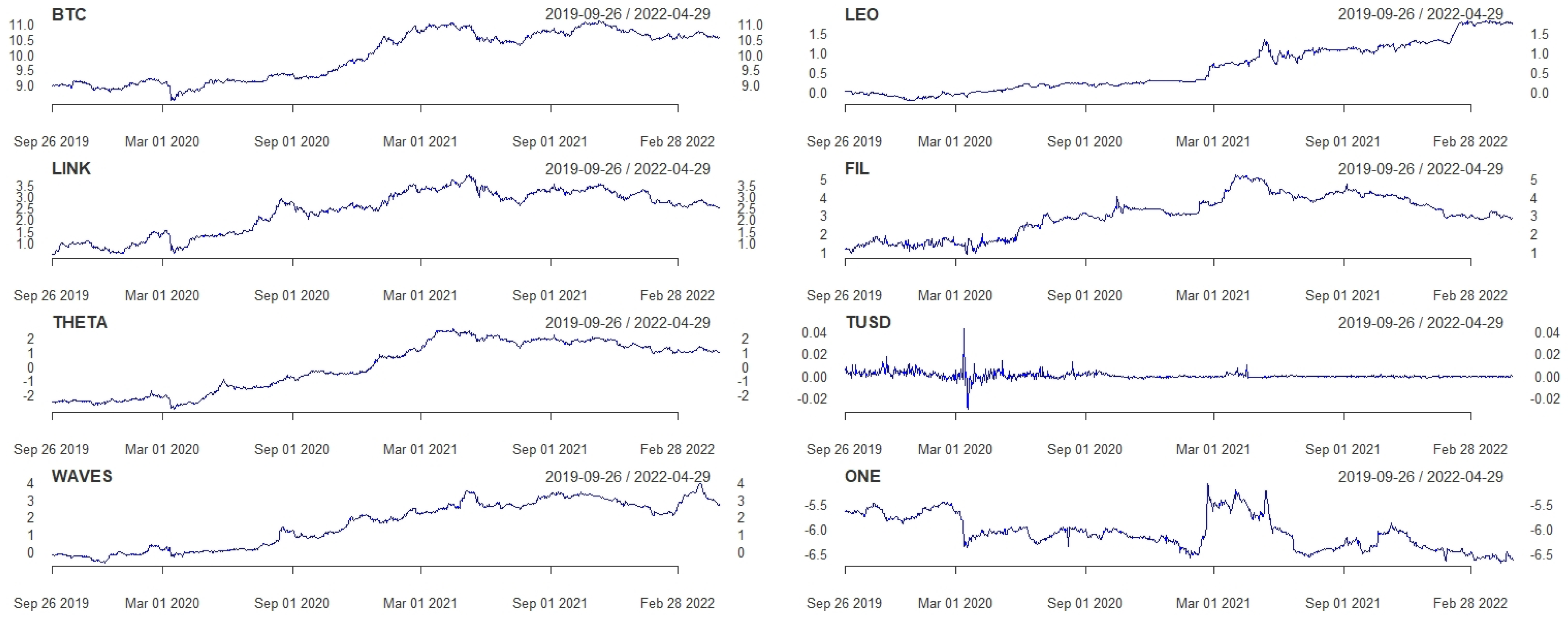
Compute log-returns of the top 100 cryptoassets.

step 2

portfolio selection

Machine learning: K-means and hierarchical clustering deployment in order to group assets that appear to be reasonably similar versus those that share large dissimilarities.

step 3

Extract Standardized Residuals from AR-GJR-GARCH(1,1) with Student-t innovations to convert the log returns into an IID series.

step 4

Use the residuals from Step 3 and standardise them with the deviations obtained in Step 3.

step 5

Convert these residuals to student-t marginals for the estimation of copula. These steps are repeated for all the cryptocurrencies to obtain a multivariate matrix of uniform marginals.

step 6

Fitting C-vine. to multivariate data obtained in step 5 and Benchmark Gauss R-vines using sequential estimation with restricted pair copula family set of first 14 copulas.

step 7

Step 6 is repeated with R-vine.

step 8

Inverse transform of the C-vine copula output using skew student-t distribution (marginal in the copula fitting).

step 9

Use outputs from step 8 to generate a series of simulated monthly portfolio returns to predict 5% CVaR.

3. Data Analysis and Empirical Results

In this section, we propose to illustrate empirically the main objective of this paper, namely, to select a diversified portfolio of cryptocurrencies using a machine learning algorithm: K-means supported by an hierarchical clustering method, investigate the performance of GJR-GARCH Differential evolution t-copula approach in modelling the co-dependence and CVaR of the selected portfolio and finally minimizing the latter risk measures in order to propose under which method a portfolio of cryptocurrencies is more risky or profitable than the other.

3.1. Data Description

We chose to apply our methodology to cryptoassets portfolios. The latter are sourced from the top 100 cryptoassets by market capitalisation (which ensures that the analysis will not be affected by liquidity risk issues) from yahoo finance (https://finance.yahoo.com/, accessed on 3 May 2022) powered by coinmarketcap (https://coinmarketcap.com/, accessed on 3 May 2022) form 1 May 2017 to 30 April 2022. We then eliminate those with less than 700 observation and this operation has produced 58 cryptoassets with 1830 daily prices. The machine learning algorithm K-means (supported by the hierarchical clustering method) is used to select a diversified portfolio of eight cryptocurrencies and cryptotokens, representing about 50% of the whole crypto-market share (see

Table 3. Description of selected cryptoassets.

Rank	Symbols	Category	Consensus Mechanism	Value Proposition	Maximum Supply (${10}^6$)	% of Total Marketcap
1	BTC	crytocurrency	PoW	digital gold	21	43.33%
20	LEO	utility token	PoS	fund reimbursement	985	0.36%
25	LINK	application token	N/A	oracle network	1000	0.65%
38	FIL	storage network	PoRep	secure decentralised	2000	1.83%
		token		storage network
48	THETA	application token	PoS	video streaming	1000	1.93%
				network
49	TUSD	stablecoin	N/A	digital fiat	N/A	0.06%
74	WAVES	application token	LPoS	Web 3.0 application &	108,325	0.13%
				decentralised solution
80	ONE	crypto-token	FBFT	deep sharding technology	12,600	1.77%

PoRep: proof-of-Replication. LPoS: Leasing Proof-of-Stake is an enhanced version of Proof-of-Stake (PoS). FBFT: Fast Byzantine Fault Tolerance.

). It is evident from Table 3 that Bitcoin reigns supreme over the cryptoassets market. As a result it controls the price formation of all altcoin.

Figure 1 and Figure 2 show respectively the evolution of the price and return dynamics for the eight cryptoassets under investigation. Visual inspection shows many signs of discrepancies than commonality signs in the returns and prices of all the eight virtual assets, testifying thus a certain dissimilarity in their behaviours over the considered period. Volatility clustering patterns are observed in the return dynamics of all eight cryptocurrencies.

The descriptive statistics of the selected cryptocurrencies examined in this paper are shown in

Table 4. Descriptive statistic.

	Dependent Variable
	BTC	LEO	LINK	FIL	THETA	TUSD	WAVES	ONE
Mean	0.169	0.185	0.215	0.178	0.368	−0.0005	0.307	−0.107
min	−46.500	−20.000	−61.500	−60.500	−60.400	−5.100	−48.700	−52.100
max	17.200	36.300	27.600	76.900	34.700	4.570	44.800	84.000
sd	4.000	3.210	6.680	10.600	7.410	0.363	7.040	5.800
asd	63.200	50.800	106.000	168.000	117.000	5.750	111.000	91.700
Kurtosis	21.700	27.300	10.900	8.980	8.410	74.800	8.280	60.100
Skewness	−1.670	1.990	−1.090	0.547	−0.770	−0.621	0.114	2.970
JB	18,528.000	29,309.000	4746.000	3161.000	2820.000	215,881.000	2651.000	140,674.000
Q10	21.200	41.900	23.900	43.100	288.000	7.190	24.800	22.200
Q102	16.100	26.700	48.500	97.000	258.000	53.300	58.300	43.100
ACF	0.040	0.035	0.086	0.210	0.077	0.473	0.116	0.080

. All currencies display positive standard deviation and mean close to zero. With the exception of LEO, FIL, WAVES and ONE coin, the other cryptocurrencies are skewed left. In addition, the Jarque–Bera (JB) test and kurtosis for each series are positive and far from zero; that is, they possess heavy tailed and non normal distribution, which is consistent with the behaviour of most financial assets.

3.2. Empirical Findings

The empirical results are analyse in three main axes: The first step of the analysis is to deploy a machine learning algorithm to form a diversified portfolio. The second step is modelling the interdependence structure of the selected cryptoassets using the C-vine and R-vine copulas and estimating the parameters of the associated pair-copula. The Last step is modelling and estimating the CVaR of the weighted portfolio of the selected cryptoassets using C-vine and R-vine copula coupled with the differential evolution algorithm.

Machine Learning: K-Means and Hierarchical Clustering

K-means in particular and clustering algorithms in general all have one common goal: to group similar items into clusters. These elements can be any type of data, as long as they are encoded in a matrix form.

Choosing a number of clusters K is not necessarily intuitive, especially when the dataset is large and the researcher does not have a priori or assumptions about the data. The elbow method is the most common for choosing the number of clusters. This method first calculates the variance which is the sum of the distances between each centroid (centre) of a cluster and the various observations included in the same cluster. Then, it seeks to find a number of clusters K so that the clusters retained minimize the distance between their centers (centroids) and observations in the same cluster, that is, minimizing the intra-class distance or total intra-cluster variance also known as total within-cluster sum of square (wss). Generally, by putting in a graph wss as a function of K like in Figure 3, one finds a graph similar to an arm where the highest point represents the shoulder and the point where K is 14, represents the other end: the hand. The optimal number of clusters is the point representing the elbow (knee). Here, the bend can be represented by K being 4 or 5. This is the optimal number of clusters. Generally, the knee point is that of the number of clusters from which the variance no longer decreases significantly.

The K-means algorithm result is recorded in

Table 5. K-means result.

Clusters	1		2				3	4
	USDP	USDC	FIL	THETHA	RUNE	LINK	LEO	ONE	BSV	XMR	NEXO	BTC
	USDT	TUSD	QNT	TFUEL	WAVES	XTZ	LUNA	TRX	NEO	DASH	DOGE	WBTC
Crypto			HOT	CHZ	FTM	MATIC		BTT	ETC	ZEC	CRO	BNB
			CEL	MANA	LRC	VET		ADA	EOS	HT	KCS	ETH
			XDC	ENJ	ATOM	ZIL		XRP	LTC	OKB	GNO	FTT
			XEM	MIOTA	BAT			XLM	BCH	DCR	MKR
wss	0.65			0.8			0.85		0.75

. The algorithm has allowed data of 58 cryptoassets to be grouped into 4 clusters, based on their similarities and dissimilarities. Cluster 1 contains 4 assets which are stablecoins having the same characteristics and behaviours. Cluster 2 contains 23 assets, mainly in the category of application token with PoS consensus mechanism or close to it, except ZIL, ICX, BAT and XVG. Cluster 3 contains 2 assets, LEO and LUNA which belong to the category of utility token PoS(Proof-of-Stake) and DPoS (Delegated-Proof-of-Stake) as consensus mechanism respectively. Cluster 4 contains 29 assets, mainly in the category of digital token with Pow (Proof-of-Work) consensus mechanism or close to it, except BNB, ETH, XRP, TRX and EOS. The dynamic of the members of this group is highly influenced by that of Bitcoin compared to the members of other groups.

The hierarchical clustering is used to confirm the results of the K-means method, and the dendrogram obtained on the basis of the intra-cluster and inter-cluster variance is depicted in Figure 4 and the level of similarity in each cluster is presented in Figure 4. As one moves up the dendrogram, assets that are similar to each other are merged into branches, which subsequently fuse at higher height. The lower the height of the fusion, the more similar the assets are and clusters with high height have greater variability within their assets.

Finally, the selection of the cryptoassets is done as follows: one stablecoin: True-USD (TUSD) is chosen in cluster 1. Since the level volatility associated to stablecoins is consistently close to zero, they are therefore “simply” a tool for dematerializing our fiat currencies, the parity of which remains stable with them and allows repeated transactions with cryptocurrencies without going through a traditional bank account. In addition, it has a negative correlation with other cryptoassets in the portfolio (see

Table 6. Correlation coefficients.

	BTC	LEO	LINK	FIL	THETA	TUSD	WAVES	ONE
BTC	1	$0.124$	$0.609$	$0.374$	$0.505$	$-0.087$	$0.465$	0.564
LOE	$0.124$	1	$0.138$	$0.035$	$0.077$	$0.055$	$0.100$	0.115
LINK	$0.609$	$0.138$	1	$0.371$	$0.487$	$-0.062$	$0.474$	0.446
FIL	$0.374$	$0.035$	$0.371$	1	$0.287$	$-0.051$	$0.263$	0.265
THETA	$0.505$	$0.077$	$0.487$	$0.287$	1	$-0.054$	$0.410$	0.339
TUSD	$-0.087$	$0.055$	$-0.062$	$-0.051$	$-0.054$	1	$-0.050$	$-0.014$
WAVES	$0.465$	$0.100$	$0.474$	$0.263$	$0.41$	$-0.050$	1	0.370
ONE	0.564	0.115	0.446	0.265	0.339	−0.014	0.370	1

). Four assets (FIL, THETA, LINK, WAVES) are selected from cluster 2 based on their higher height of dissimilarity (low correlation) with Bitcoin. In cluster 4, Harmony (ONE) is the most dissimilar coin to Bitcoin (see Figure 2 and Figure 4), so both are chosen.

3.3. Modelling the Residual Dependencies Using Vine Copula

Econometric models coupled with vine copula are commonly used in the field of multivariate modelling of financial returns. The GARCH marginal time series model is first fitted to each cryptoasset returns and standardised residuals are formed. These residuals are subsequently transformed to marginally uniform data using parametric probability integral transformation and used as inputs for the selection of the appropriate bivariate copula. The Alkaike information criterion (AIC) is used to select the copula that best fits the data.

At the first step the univariate AR(1, 1)-GJR-GARCH(1, 1) model with Student-t innovations is fitted to the log return series of each cryptoasset to extract standardised residuals and their independence are verified using the Ljund-Box test. Subsequently, the empirical probability integral (since the data size is large) is used to transform the standardised residuals to obtain marginally uniform data (iid residuals) for the estimation of copula. These steps are repeated for the eight cryptoassets to obtain a multivariate matrix of uniform marginal. The selected bivariate copula and their estimated Kendall’s tau for the eight cryptoassets are recorded in

Table 7. Parameter estimate of C-vine copula.

Tree	Edges	Copula	par1	par2	Kendall’s $\mathit{\tau }$	utd	ltd
1	BTC-TUSD	G90	0.02	–	−0.06	–	–
	BTC-FIL	SG	0.03	–	0.27	–	0.35
	BTC-LEO	t	0.03	2.00	0.09	0.03	0.03
	BTC-THETA	SBB7	0.07	0.07	0.38	0.04	0.57
	BTC-WAVES	SJ	0.06	-	0.33	-	0.56
	BTC-LINK	SBB6	0.19	-	0.45	-	0.6
	ONE-BTC	SG	0.05	–	0.41	–	0.49

for C-vine and

Table 8. Parameter estimate of R-vine copula.

Tree	Edges	Copula	par1	par2	Kendall’s $\mathit{\tau }$	utd	ltd
1	LINK-LEO	t	0.03	2.37	−0.09	0.02	0.02
	BTC-TUSD	G90	0.02	–	−0.06	–	–
	LINK-FIL	SG	0.03	–	0.27	–	0.34
	BTC-THETA	SBB7	0.07	0.07	0.38	0.04	0.57
	LINK-WAVES	SBB8	0.06	0.00	0.33	–	–
	BTC-LINK	SBB6	0.19	0.15	0.45	–	0.60
	ONE-BTC	SG	0.05	–	0.41	–	0.49

showing different strengths and signs of pairwise dependencies.

3.3.1. Canonical Vine Copula

Figure 5 represents the structure of the C-vine. The node that maximises the sum of pairwise dependencies is chosen as the root of the tree. In tree 1 all altcoins are connected to Bitcoin. This confirms the leading role Bitcoin plays in the price formations of other cryptoassets, as it accounts for about 44% of the total crypto-market shares.

A range of 14 bivariate copula functions was available for selection to model the dependences. The following four copula functions were selected based on the AIC criterion (key characteristics are given in

Table 9. Characteristic of copula functions.

Name	Dependence Structure	Strength	Weakness
S. Gumbel (SG)	only negative	lower tail dependence	upper tail dependence
S. Joe (SJ)	only negative	lower tail dependence	upper tail dependence
Rotated 270 Gumbel (G270)	only negative	tail-asymmetry	no tail dependence
S. Joe-Gumbel (SBB6)	independent or positive	tail symmetric
S. Joe-Clayton (SBB7)	independence or negative	lower tail dependence	upper tail dependence
S. Joe-Frank (SBB8)	positive or negative	symmetrical & tail dependence

): Survival Joe-Gumbel and Clayton (SBB6, SBB7), survival Gumbel or rotated Gumbel by 180 degree (SG), survival Joe (SJ), student-t and rotated Gumbel by 90 degree (G90): The predominance of survival and mixed copula indicate the presence of lower-tail dependences (ltd) which characterise cryptoasset markets during extremes. The structure in Figure 5 reflects the expected relationship among cryptoassets. The resulting pairs of cryptoassets captured by the appropriate copula are recorded in Table 7 together with their corresponding estimated parameters and Kendall’s tau values indicating different strengths of dependencies. We observe from the Kendall’s tau column that Bitcoin is positively and moderately correlated with altcoins except with True USD with whom it has a strong negative correlation (with the negative correlation with BTC, whom is positively correlated with other altcoin. True USD can be used for hedging during market turmoil).

3.3.2. Regular Vine Copula

Since R-vine copula by construction is more flexible than C-vine, we propose in this section to deploy R-vine to the eight selected cryptoassets and compare the result to that of C-vine. Figure 6 shows tree 1 for R-vine and the flexibility can be seen at first glance. Two categories of cryptoassets emerge from tree 1, LINK, ONE, THETA and TUSD are the most connected to Bitcoin and LEO, FIL and WAVES are most connected to LINK but have no direct dependency with Bitcoin. This subdivision clearly underscores the flexibility of R-vine structure over that of C-vine and can be partly explained by the fact all the altcoin directly connected to LINK are application token and with almost the same consensus mechanism. We observe from Table 8 that tree 1 of R-vine, three mixed copula families (SBB6, SBB7, SBB8) compared to two mixed copula (SBB6, SBB7) for C-vine. This shows the power of R-vine to capture complex dependencies.

Examining Table 7 and Table 8 we observe that edges that are similar to C-vine and R-vine have been captured by the same rotated or survival copula functions and have equal dependency strength (Kendall’s tau). In addition, the results in the last two columns of both tables show the evidence of capturing fat-tailed distribution and left tail risk in economic and financial downturns as SG, SBB6,7,8 copula, which capture lower, asymmetric and symmetric behaviour are dominant.

Comparison results between C-vine and R-vine copula is summarised in

Table 10. Model comparison.

	loglik	AIC	BIC	Number of Copula Types on Tree1
C-Vine	1240	−2435	−2324	6
R-vine	1238	−2427	−2311	6

. The log-likelihood obtained after optimisation of the chosen copula type are in column 1. The Akaike’s Information Criteria (AIC) and Bayesian Information Criteria are recorded in columns 2 and 3, respectively. We observe that the values of those three comparison factors for C-vine are greater than the ones of R-vine. Overall, this result shows the usefulness of C-vine copulas with individually selected type of copulas for each term of the pair-copula. In addition, the selection procedure of C-vine gives a result that is consistent with crypto-market dynamics.

3.4. Portfolio Optimisation

Table 11. Cvine: weighs.

Rebal Periods	BTC	LEO	LINK	FIL	THETA	TUSD	WAVES	ONE
month 1	0.09	0.22	0.02	0.16	0.14	0.22	0.09	0.06
month 2	0.04	0.31	0.10	0.13	0.06	0.24	0.02	0.10
month 3	0.09	0.33	0.02	0.10	0.08	0.20	0.07	0.11
month 4	0.11	0.22	0.06	0.17	0.03	0.21	0.08	0.12
month 5	0.02	0.29	0.02	0.10	0.05	0.25	0.08	0.19
month 6	0.12	0.33	0.02	0.12	0.08	0.20	0.06	0.07
month 7	0.10	0.29	0.02	0.22	0.02	0.02	0.05	0.10
month 8	0.03	0.20	0.06	0.18	0.10	0.27	0.02	0.14

shows a fairly weighted (between 0 and 0.33) portfolio, with LEO and TUSD having the largest weight throughout the various period. This is consistent with the fact that, the return dynamic of LEO is opposite to the one of Bitcoin (see Figure 2) and can therefore be used together with a stablecoin such as TUSD to mitigate or hedge against the risk. FIL and Bitcoin are the third and fourth weighted assets across the considered period for optimal return. The less weighted assets are LINK, THETA and WAVES which belong to the same category of application token and are strongly correlated in the lower tail (see Table 7) with Bitcoin, making them more riskier than the remaining assets. This may justify their lower weight allocation.

The optimisation result in

Table 12. CVine: CVaR and mean.

Rebal Periods	CVaR	Mean
month 1	0.720	0.0421
month 2	0.732	0.0405
month 3	0.718	0.0415
month 4	0.731	0.0414
month 5	0.740	0.0415
month 6	0.740	0.0382
month 7	0.747	0.0406
month 8	0.750	0.0434

shows that the CVaR is high across all the period which is in line with the well-known fact that cryptomarket is highly volatile. This an improvement as compared to previous studies exhibiting a CVaR over 100%. We can also observe that the CVaR is almost constant throughout the period and the same movement can be noticed for the mean return with about 4% per period. It seems less than expected, but remains constant. An investor looking for a portfolio which can generate a fixed cash flow rather than the returns that fluctuate between gains and losses across period, should consider such portfolio.

4. Conclusions

The goal sought through this paper was to develop a method that could allow a crypto-investor or manager to select a diversified portfolio of cryptocurrencies and to estimate the risk and profitability of the portfolio. Our approach to diversification combined similarity and tail dependence structure through K-means algorithm and Vine copula respectively, thus, achieving wealth/weights allocation which is not concentrated only on few assets.

During this study, we first tried to illustrate a method that relies on the K-means algorithm and which made it possible to select a diversified portfolio of eight cryptocurrencies. Subsequently, we opted for a GARCH-C-Vine copula approach combined with the differential evolution algorithm for co-dependence analysis in order to estimate the return and CVaR of the selected portfolio. The method also makes it possible to determine an accurate and reliable result in a very short computing time, which facilitates its implementation in practice. Our results show:

• consistency with the risky characteristics of the cryptocurrency market-unregulated, anonymity of the transaction and highly volatile.
• that stablecoin such as True-USD is negatively correlated to the other cryptoassets in the portfolio and could therefore be safe haven for crypto-investors during market turmoil.

On the other hand our findings are in line with previous studies exhibiting stablecoins as potential diversifiers.

Contrary to the previous studies which focused mainly on the top twenty, we build our portfolio from a pool of hundred cryptocurrencies to take advantage of possible dissimilarity that may exists among them. The top twenty cryptocurrencies considered in previous studies appear to be be highly correlated, so that a diversified cryptocurrency portfolio cannot be formed from these top twenty.

Several extensions of this work can be considered later. For example, it would be interesting to consider the use of diversification measures such as Diversification ratio or Entropy. The higher these measures, the well diversified a portfolio will be. We could also consider a diversification approach through risk contribution with risk measures being either CVaR or any other coherent risk measures such as spectral risk measure or distortion risk measure. One could also consider a possibility of a multi-period horizon for the portfolio optimisation with rebalancing with additional constraints such as transaction costs.

References

1. Markowitz, H. Portfolio selection. J. Financ. 1952, 7, 77–91. [Google Scholar]
2. Markowitz, H. Portfolio Selection: Efficient Diversification of Investments; John Wiley and Sons: Hoboken, NJ, USA, 1959. [Google Scholar]
3. Bares, P.; Gibson, R.; Gyger, S. Hedge Fund Allocation with Survival Uncertainty and Investment Constraints. Soc. Sci. Res. Netw. 2002, 1–50. [Google Scholar] [CrossRef] [Green Version]
4. Javed, F.; Mazur, S.; Ngailo, E. Higher order moments of the estimated tangency portfolio weights. J. Appl. Stat. 2021, 48, 517–535. [Google Scholar] [CrossRef] [PubMed] [Green Version]
5. Khan, K.I.; Naqvi, S.M.W.A.; Ghafoor, M.M.; Akash, R.S.I. Sustainable Portfolio Optimization with Higher-Order Moments of Risk. Sustainability 2020, 12, 2006. [Google Scholar] [CrossRef] [Green Version]
6. Jurczenko, E.; Maillet, B.; Merlin, P. Hedge Funds Portfolio Selection with Higher-Order Moments: A Non-Parametric Mean-Variance-Skewness-Kurtosis Efficient Frontier; Social Science Research Network (SSRN): Rochester, NY, USA, 2005. [Google Scholar]
7. Hunjra, A.I.; Alawi, S.M.; Colombage, S.; Sahito, U.; Hanif, M. Portfolio Construction by Using Different Risk Models: A Comparison among Diverse Economic Scenarios. Risks 2020, 8, 126. [Google Scholar] [CrossRef]
8. Krokhmal, P.; Palmquist, J.; Uryasev, S. Portfolio optimization with conditional value-at-risk objective and constraints. J. Risk 2002, 4, 43–68. [Google Scholar] [CrossRef] [Green Version]
9. Agarwal, V.; Naik, N.Y. Risks and portfolio decisions involving hedge funds. Rev. Financ. Stud. 2004, 17, 63–98. [Google Scholar] [CrossRef]
10. Babaei, S.; Sepehri, M.M.; Babaei, E. Multi-objective portfolio optimization considering the dependence structure of asset returns. Eur. J. Oper. Res. 2015, 244, 525–539. [Google Scholar] [CrossRef]
11. Mba, J.C.; Pindza, E.; Koumba, U. A differential evolution copula-based approach for a multi-period cryptocurrency portfolio optimization. Financ. Mark. Portf. Manag. 2018, 34, 399–418. [Google Scholar] [CrossRef]
12. Boako, G.; Tiwari, A.K.; Roubaud, D. Vine copula-based dependence and portfolio value-at risk analysis of the cryptocurrency market. Int. Econ. 2019, 158, 77–90. [Google Scholar] [CrossRef]
13. Mba, J.C.; Mwambi, S. A Marvov-Switching COGARCH approach to cryptocurrency portfolio selection and optimization. Financ. Mark. Portf. Manag. 2020, 34, 199–214. [Google Scholar] [CrossRef]
14. Sklar, A. Functions de Répartition a n dimensions et leurs Marges. Publ. Inst. Stat. L’Université Paris 1959, 8, 229–321. [Google Scholar]
15. Joe, H. Multivariate Models and Dependence Concepts; Chapman & Hall: London, UK, 1997. [Google Scholar]
16. Bedford, T.; Cooke, R.M. Probability density decomposition for conditionally dependent random variables modeled by vines. Ann. Math. Artif. Intell. 2001, 32, 245–268. [Google Scholar] [CrossRef]
17. Bedford, T.; Cooke, R. Vines—A new graphical model for dependent random variables. Ann. Stat. 2002, 30, 1031–1068. [Google Scholar] [CrossRef]
18. Glosten, L.R.; Jagannathan, R.; Runkle, D.E. On the relation between the expected value and the volatility of the nominal excess return on stocks. J. Financ. 1993, 48, 1779–1801. [Google Scholar] [CrossRef]
19. Storn, R.; Price, K. Differential Evolution—A Simple and Efficient Adaptive Scheme for Global Optimization over Continuous Spaces; TR-95-012; Intemational Computer Science Institute (ICSI): Berkeley, CA, USA, 1995. [Google Scholar]
20. Ababio, K.A.; Mba, J.C.; Koumba, U. Optimisation of mixed assets portfolio using copula differential evolution: A Behavioural approach. Cogent Econ. Financ. 2020, 8, 1780838. [Google Scholar] [CrossRef]
21. Das, M.; Roy, A.; Maity, S.; Kar, S.; Sengupta, S. Solving fuzzy dynamic ship routing and scheduling problem through new genetic algorithm. Decis. Making Appl. Manag. Eng. 2021. [Google Scholar] [CrossRef]
22. Rockafellar, R.T.; Uryasev, S. Optimization of conditional value-at-risk. J. Risk 2000, 2, 21–42. [Google Scholar] [CrossRef] [Green Version]
Figure 1. Cryptoasset prices evolution from May 2017 to April 2022.
Applsci 12 06408 g001
Figure 2. Cryptoasset returns in the sample spanning from May 2017 to April 2022.
Applsci 12 06408 g002
Figure 3. Elbow method result for determining the optimal number of clusters.
Applsci 12 06408 g003
Figure 4. Dendrogram of the cryptoassets.
Applsci 12 06408 g004
Figure 5. C-vine tree 1.
Applsci 12 06408 g005
Figure 6. R-vine tree 1.
Applsci 12 06408 g006