Abstract
In this study, a numerical simulation model and an analytical method are introduced to evaluate the particle collection efficiency and transport phenomena in an electrostatic precipitator (ESP). Several complicated physical processes are involved in an ESP, including the turbulent flow, the ionization of gas by corona discharge, particles’ movement, and the displacement of electric charge. The attachment of ions charges suspended particles in the gas media. Then, charged particles in the fluid move towards the collection plate and stick on it. The numerical model comprises the gas flow, electrostatic field, and particle motions. The collection efficiency of the wire-plate type ESP is investigated for the particle diameter range of 0.02 to 10 µm. It is observed that electric field strengths and current densities show considerable variation in the solution domain. Meanwhile, changing supply voltage and charging wire diameters significantly affect the acquired charges on the electrostatic field and particle collecting efficiencies. Simultaneously, the distance between the charging and collecting electrodes and the main fluid inlet velocity has an important effect on the particle collection efficiency. The influence of the different ESP working conditions and particle dimensions on the performance of ESP are investigated and discussed.
1. Introduction
The harmful emissions of micro and nanoparticles to the environment inevitably increase with technological development. These contaminants significantly affect human health as well as the environment and organisms [1,2,3,4]. There are various contaminant filtering technologies; among them, electrostatic precipitation has the advantages of low-pressure drop in the main fluid flow and relatively good performance in the collection efficiency [5,6,7]. Electrostatic precipitation systems have been widely used to control the emissions with flue gases in power generation systems, combustion and chemical processing units, and several industrial mass transport processes. They have also been employed to clean the contaminated indoor air, in which various gases and particulate matter exist [5,8]. The wire-plate type of electrostatic precipitators (ESP) is widely used in several applications. The numerical modelling of an ESP requires detailed electric field solutions incorporating flow field and particle transport modelling.
The primary operating mechanism behind the electrostatic precipitators is that volatile particles that flow through the channel are charged by a high-voltage supply electrode, then charged particles are attracted toward the collection electrodes by Coulomb forces and trapped on them. The electrostatic precipitation mechanism has three essential steps, namely [5]:
- Particle charging,
- Particle collection,
- Removal of the collected dust.
Many factors significantly affect the operation of the ESP. The applied voltage is the most critical parameter because it determines the electrostatic field and thus corona discharge [9,10]. The gas speed identifies the residence time of particles in the ESP and encompasses a direct impact on particle charging [9,11]. Inlet height, wire spacing. and the precipitator arrangement may influence the gas velocity and particle charging in a wire-plate ESP [12].
Electrostatic precipitators (ESP) are commonly used in industrial facilities. The main drawback of ESP technology is its high sensitivity to operating conditions [13]. Therefore, it is necessary to investigate the performance of ESPs under various operating conditions. Experimental investigation of ESPs is costly and extraordinarily complex; therefore, simulation tools are commonly preferred [14]. Nevertheless, due to the complexity of ESPs, a complete numerical model is not available. CFD is an alternative method to study the behavior inside the ESP [15]. There are various studies in the literature to model ESP behavior using CFD tools. A few numerical strategies have been improved to simulate the flow field of primary fluid and particles, the electric field in the ESP, and the space charge density including the finite volume method [16], the boundary element method [17,18], and the finite differencing technique [19]. The researchers also examined the impact of various operating conditions and ESP geometries on collection efficiency [20,21,22,23]. In another study, Wen et al. (2016) presented a numerical model to explain the particle transport, flow field, and electric field of guidance-plate-covered ESPs [24]. The study revealed that, compared to traditional ESPs, ESPs with particle trapping mechanisms such as guidance plates have higher collection efficiencies as the dust has a lower chance of returning to the environment. Park et al. (2018) developed a simulation model to simulate turbulent flow, particle trajectory, and particle charging for single-stage ESPs [25]. Collection efficiencies and particle charging were investigated for different flow speeds, voltages, and particle sizes. Tu et al. (2017) investigated the collection efficiency of a hybrid electrostatic filter with perforated plates both experimentally and numerically [26]. Simulation results were found in good agreement with the experimental results. However, these specified calculation methods are usually not accessible or open to the usage of researchers who are working in the same area. Therefore, limited numerical modelling research is reported regarding the essential connections between electrostatic field properties, collection efficiency (ESP performance), and ESP design.
This research is aimed to present a detailed three-dimensional numerical model of an electrostatic precipitator (ESP). The numerical model comprises the gas flow, electrostatic, and particle motions in the solution domain. The model is employed to evaluate the turbulent airflow, particle charging, and transport behaviors in the solution domain. The collection efficiency of the wire-plate type ESP is also investigated in this interacting media, including electric field, fluid dynamics, and particle dynamics. In addition to the numerical model, an improved analytical model proposed a generalized and relatively easy estimation procedure for the ESP collection efficiencies of an extensive range of particles between 20 nanometers and 10 μm. The numerical model is also used to validate the analytical model collection efficiency results. The different geometric and operational parameters, including the particle properties, are considered to obtain the collection efficiency of the ESP.
2. Materials and Methods
The air in the ESP is assumed as incompressible, and the airflow is considered turbulent. A corona discharge develops under the effect of an electrostatic field. Created ions cling to suspended particles. As a result, the electrostatic force is exerted on charged particles, which impacts air and charged particle movement. Under the Eulerian framework, the governing equations explaining airflow can be stated as follows:
where xi is the coordinate component, ui is the fluid velocity component (m/s), ρ is the fluid density (kg/m3), μ is the dynamic viscosity (kg/ms), μt is the turbulent viscosity (kg/ms), ρion is the ionic charge density (C/m3), p is the pressure (Pa), and Ej is the electric field strength (V/m). The electrostatic force is described by the third term on the right-hand side of Equation (2). The electric field strength and ion charge density are required for its description. Sc represents the other source terms. The electric field strength is defined as follows:
where ϕ is the electric potential (V); the Poisson equation can be used to describe the electric potential in the ESP.
where ε0 is the permittivity of air and ρp is the particle space charge density (C/m3). On the other hand, the movement of particle charge is affected by the airflow and the electric field. The current continuity equation and current density (Ji) can be described as follows:
where Di is the ion diffusion coefficient (m2/s) and bion is the ion mobility (1.5 × 10⁻⁴ (m2/Vs) of positive charging).
Steady-state Reynolds Averaged Navier–Stokes and energy equations are solved. Turbulence is modelled with the two-equation RNG k-ε approach, which was used and validated in the previous studies such as [27,28]. At the input, the fluid velocity, turbulence intensity, and turbulent viscosity ratio are provided. At the outlet, the pressure is indicated. At all walls, a no-slip condition is applied. At the wire electrode, the electric potential is specified as the operating potential. At the particle collecting plate, the electric potential is set to zero. At all other boundaries, the gradient of the electric potential is zero. At the inlet, outflow, and particle collection plate, the gradient of ion charge density is zero. The ion charge density is calculated as assuming that the charge density is uniform in the corona region. Hence, the following Peek’s equation was satisfied on the corona wire surface.
where f is the roughness factor (assumed as one in this study), T is fluid temperature (K), P is operating pressure (kPa), T0 and P0 are temperature and pressure at the reference state of 101 kPa and 293 K, and rw is the radius of the corona wire.
The particle transport equation can be derived by applying the conservation of momentum for the particles. Then, the particle momentum equation may be given as in Equation (8):
where up represents the particle velocity (m/s), mp is the particle mass (kg), F represents the force acting on the particle (N), subscripts d, g, c, s, b, th, pg, and vm indicate drag, bouncy, Coulomb, Saffman lift, Brownian, thermophoretic, pressure-gradient, and virtual-mass forces, respectively. When a particle moves in a fluid environment, several forces, named as drag force Equation (9), bouncy force Equation (11), electrostatic body force (Coulomb force) Equation (12), Saffman lift force Equation (13), Brownian force Equation (14), thermophoretic force Equation (15), pressure-gradient force Equation (16), and virtual mass force Equation (17), may act on the particle. Detailed information about these forces can be found in the reference [29].
where dp is the particle diameter; ρp is the particle density (kg/m3); Cc is the slip correction factor defined as follows [30]:
where λ is the mean free path of air (0.066 µm at 101 kPa and 293 K) [31].
where qp is the electrical charge of a particle (=npe; np is the charge number of a particle, and e is the charge of an electron (C)).
where dij is the deformation tensor. Amplitudes of the Brownian force components are given in Equation (13).
where kB is the Boltzmann constant (1.38 × 10⁻²³ J/K), are zero-mean, unit-variance-independent Gaussian random numbers, T is the fluid temperature (K), and ν is the fluid kinematic viscosity (m2/s).
Kn is the Knudsen number (2λ/dp), kr is the ratio of fluid heat conductivity to particle heat conductivity (k/kp), μ is the fluid viscosity. Cs, Ct, and Cm coefficients were taken as 1.17, 2.18, and 1.14, respectively.
Particles in the contaminated air are charged by means of ions generated by corona discharge. A number of researchers have developed the particle charging theory. The field-modified diffusion model (FMD) presented by Ref. [32] has been widely employed to determine particle charge. This model considers both diffusion and field charging. It is derived as a linear differential equation of first-order, which can be solved with respect to time. Therefore, the FDM model proposed by Ref. [32] is employed in the present numerical model.
In the Equations (18)–(22), v, w, and tp are dimensionless particle charge, dimensionless electric field, and dimensionless particle charging time, respectively. εp is the relative permittivity of the particle.
The particle trajectory equations Equation (8), and other complementary equations describing heat or mass transfer with the particle, are solved by employing the discrete phase module (DPM) of Fluent [33]. DPM applies stepwise integration over discrete time steps at each point along with the particle path to obtain the particle’s velocity. Details of the DPM theory and usage can be found in the Ansys Fluent 19.0 Theory Guide [29].
Electrostatic field and particle charging modelling have been implemented to the Fluent by using the user-defined functions (UDF) incorporating with user-defined scalar (UDS) and user-defined memory (UDM) functions. Details of the UDF usage can be found in the Ansys Fluent 19.0 Theory Guide [29]. The commercial software ANSYS Fluent 19.2 is used to solve all governing equations. The pressure-velocity coupling is handled using the SIMPLE algorithm. The second-order upwind technique is used to discretize all convection terms. When the normalized residuals are less than 10−5, the computation is assumed convergent.
2.1. Validation of Numerical Model
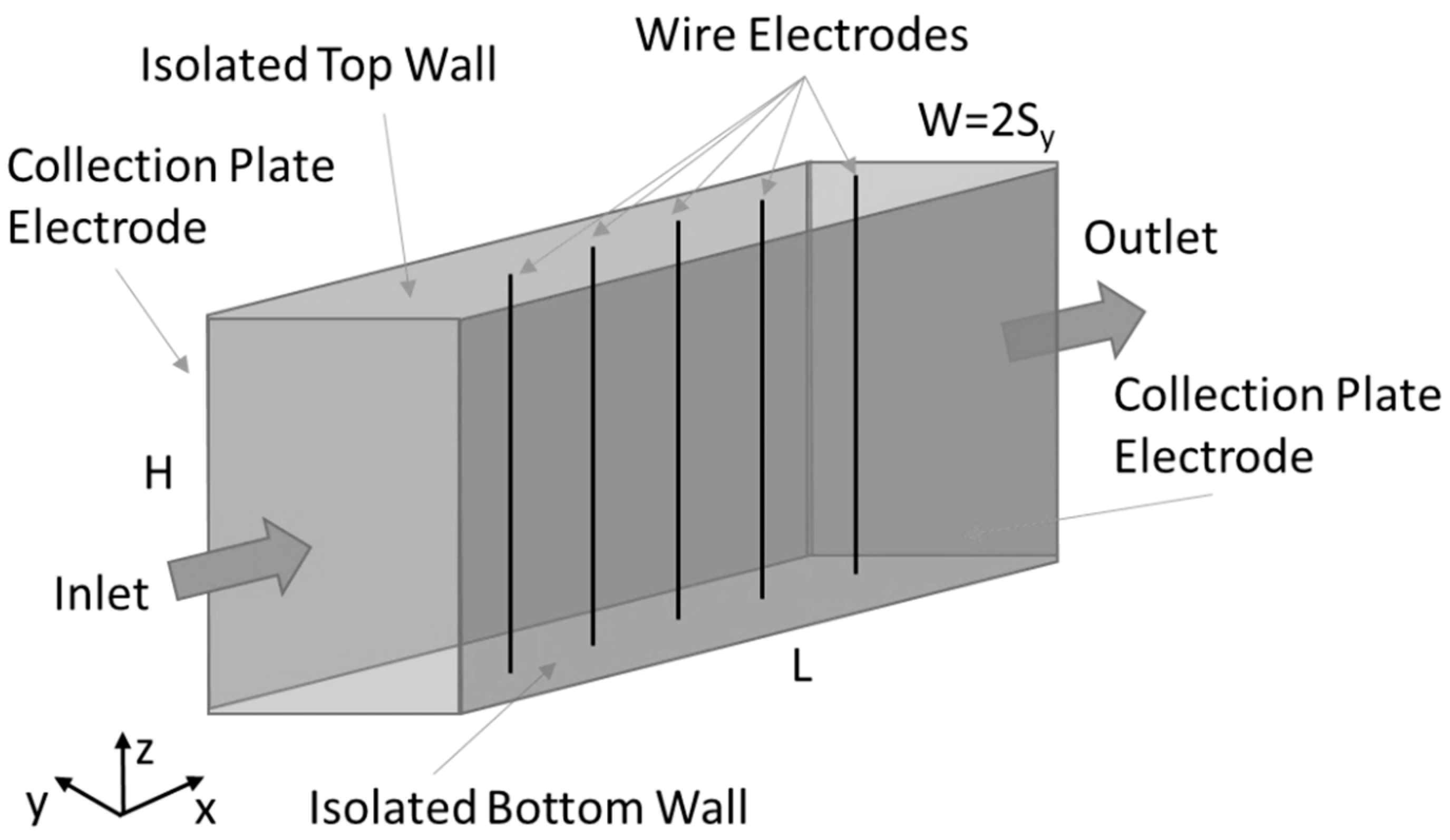
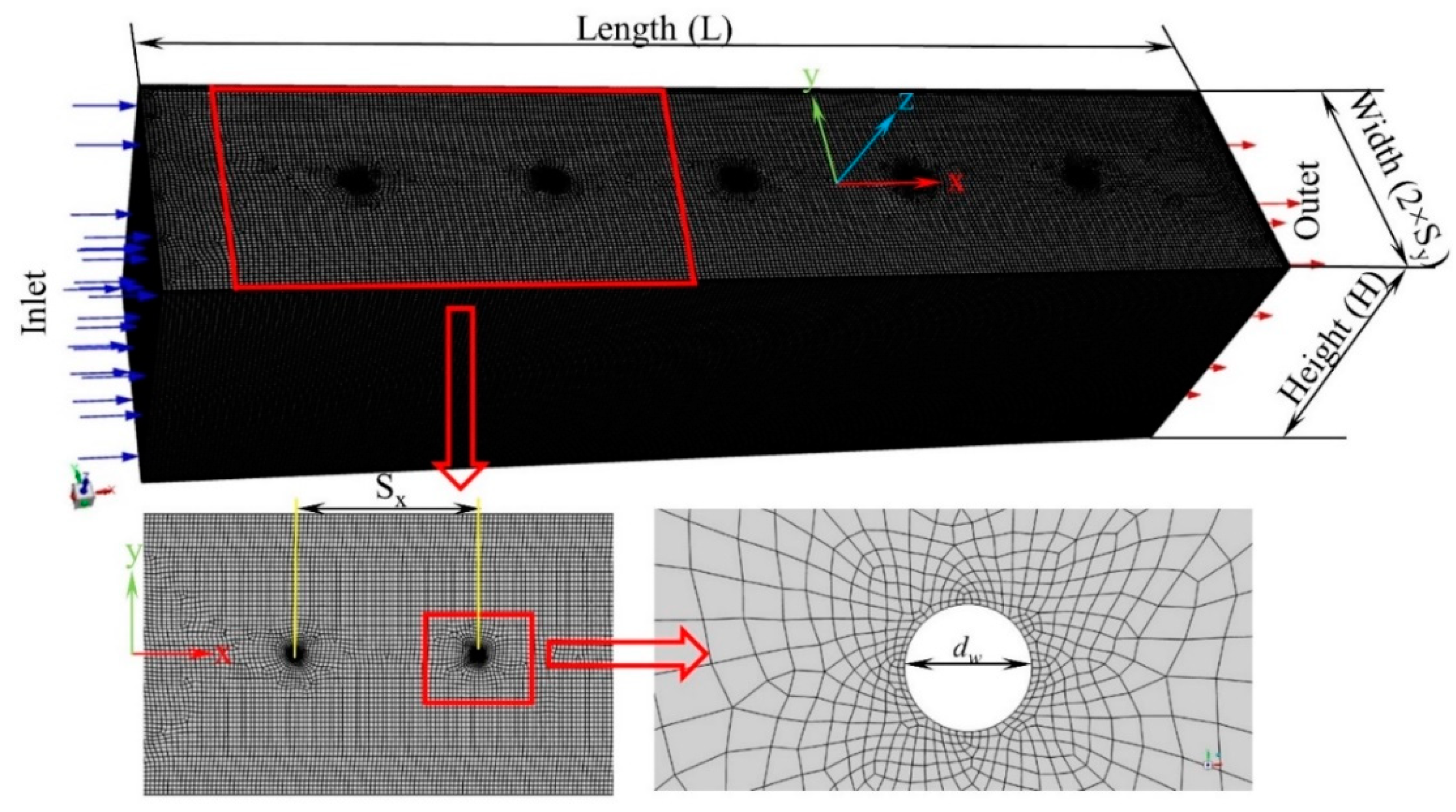
Validation of the numerical model is performed with the available experimental data in the literature. The schematic of the ESP system used in the present study is illustrated in Figure 1. Mesh structure and the geometric parameters are given in Figure 2. Considering the variations of the electrical variables near the wire electrodes, high mesh intensity surrounding the wires were generated. Consequently, the generated mesh was a much denser vicinity of the wire electrodes to increase the accuracy of the calculated gradients in the high current density zones. Since the mesh structure significantly affects the accuracy of the results and the solution time, a grid dependence test was also performed. It is found that about two million elements in total are enough for the grid-independent analysis. The solution domain was discretized with tetrahedral and hexahedral cells. These structures are adjusted with the available experimental data given in the literature.

Figure 1.
Schematic of the ESP model.
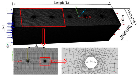
Figure 2.
Mesh structure and geometric parameters.
The single-channel ESP system consisted of a simple channel with two plate grounded electrodes, and five discharge supply wire electrodes were used for the validation of the present simulation model. The discharge supply electrodes were placed in the midplane of the channel along the positive y-direction, with the flow of the particle-injected gas in the positive x-direction (Figure 1). The total length of the rectangular ESP channel was 900 mm length with a width of either 230 mm or 180 mm. The discharge supply electrodes that were modelled had a diameter of 0.3, 1, and 2 mm with a length of 300 mm.
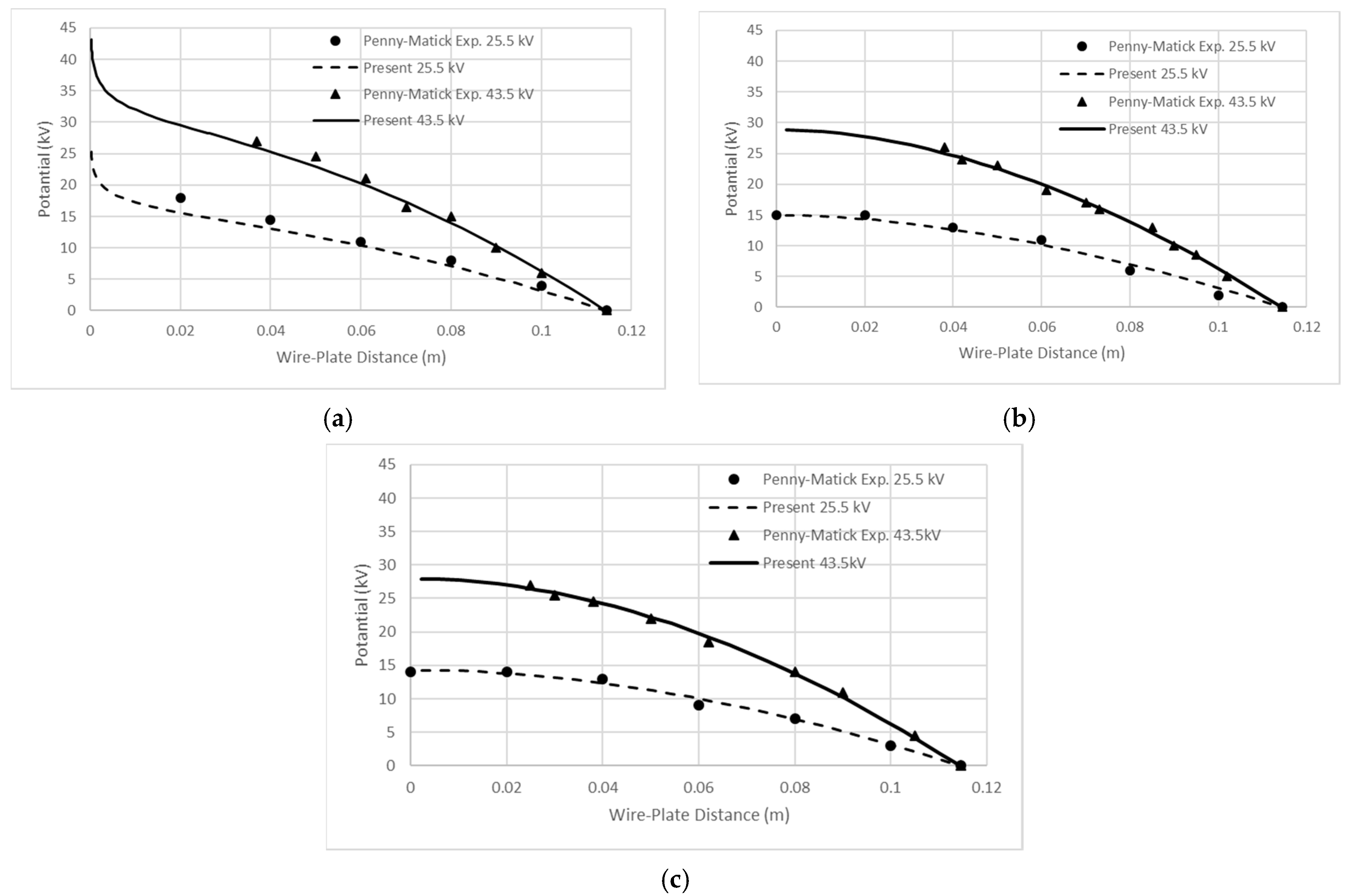
The present numerical model is validated against the experimental measurement data of Penny and Matick [34]. The operating voltages are 25.5 and 43.5 kV, the corona wires diameter is 0.305 mm, the distance between the wire and the plate is 115 mm, and the distance between the wires (Sx) is 152 mm. The comparative results of the model verification study for the potential variations between the wire and plates are shown in Figure 3. Figure 3a shows the potential variation versus the distance from the wire electrode to the collection plate. Figure 3b shows the potential variation versus the distance from the midplane (at the point of a quarter distance between the wires) to the collection plate. Figure 3c shows the potential variation versus the distance from the midplane (at the middle point between the wires) to the collection plate. In general, the current simulation agrees well with the experimental results. It demonstrates that the existing model is very good at simulating the electric field distribution in the ESP.
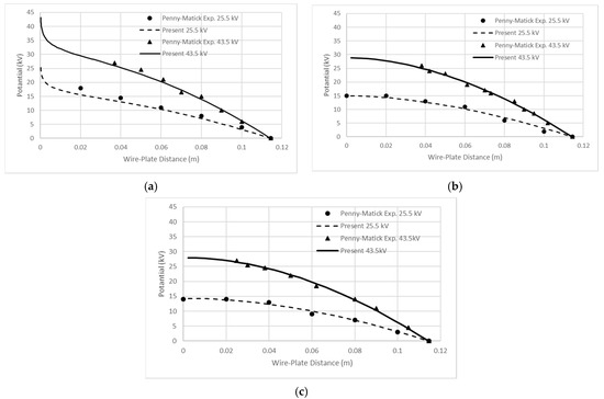
Figure 3.
Comparison of electric potential values with experimental data: (a) at x = 228.6 mm, (b) at x = 266.7 mm, and (c) at x = 304.8 mm.
The present model is also validated against the experimental data of Kihm [35]. The experimental set-up had eight corona discharge wires. The operating voltages vary between 6 and 13 kV. Each corona wires’ diameter (dw) is 0.1 mm, the distance between the wire and the plate (Sy) is 25 mm, the distance between the wires (Sx) is 50 mm, and the length (L) and height (H) of plates are 400 mm and 50 mm, respectively. Particle density (ρp) and relative dielectric constant (εp) are 893.5 kg/m3 and 2.5. The injected particles’ diameter is 4 µm. Gas velocity (Uin) is 2 m/s. Particles are injected into the computational domain from the inlet surface, and the motions and charging process of particles were calculated once through the domain. Collection efficiency as a function of the particle diameter was obtained as follow:
where Nc represents the trapped particles on the collection plates, Ntot defines the total number of particles injected into the channel. Figure 4 shows the comparison of the present model computation of the collection efficiency values with the experimental data of Kihm [35]. It can be seen that the present simulation obtains good agreement with the experimental data.
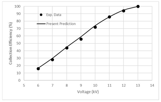
Figure 4.
Comparison of collection efficiency values with the experimental data.
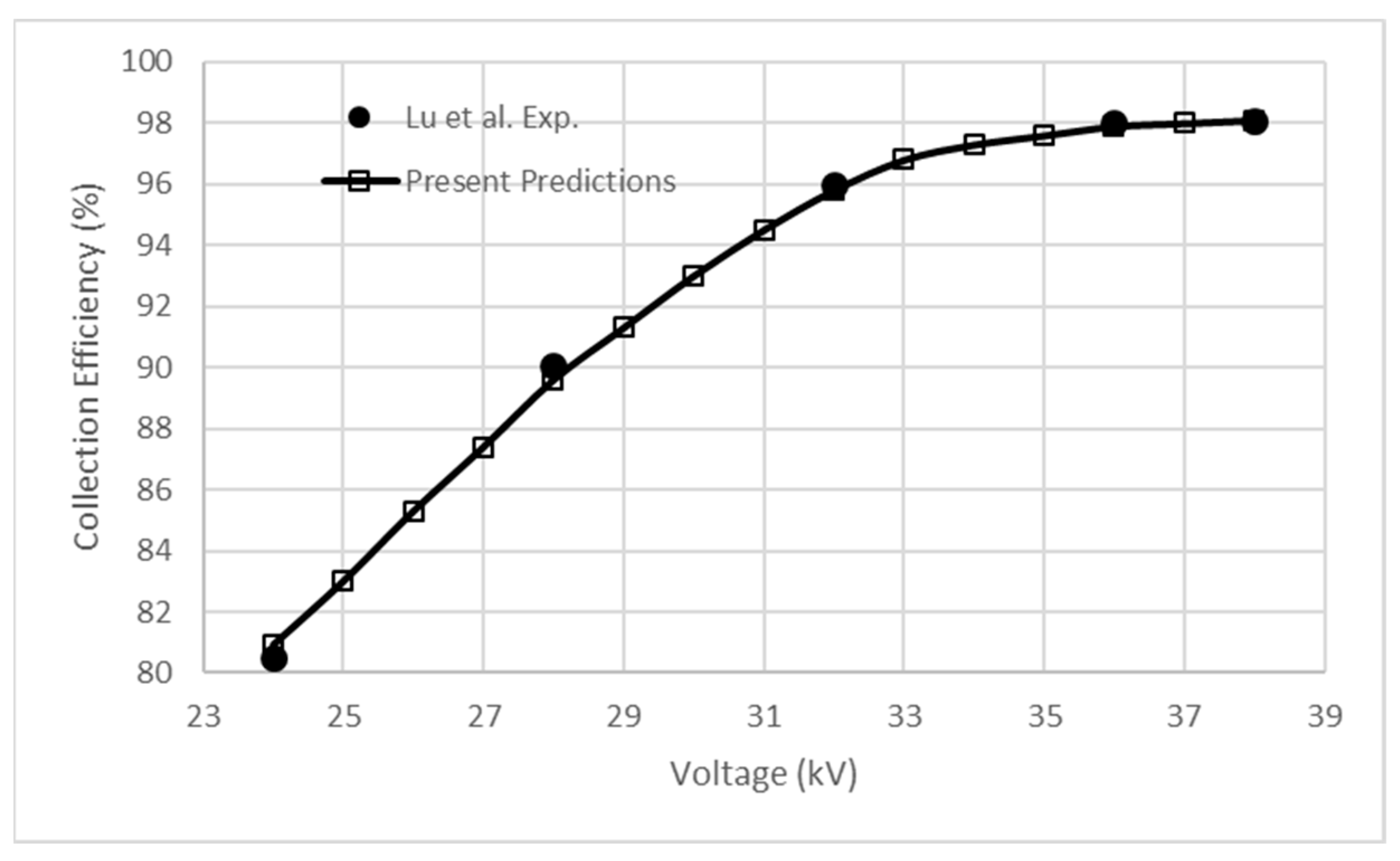
The present model is also validated against the experimental data of Ref. [9]. The experimental set-up had eight corona discharge wires. The operating voltages vary between 24 and 38 kV. Each corona wires’ diameter (dw) is 0.1 mm, the distance between the wire and the plate (Sy) is 120 mm, the distance between the wires (Sx) is 250 mm, the length (L) and height (H) of plates are 1200 mm and 150 mm, respectively. Particle density (ρp) and relative dielectric constant (εp) are 600 kg/m3 and 2.5. The injected particles’ diameter is 5 µm. Gas velocity (Uin) is 0.4 m/s. Figure 5 shows the comparison of the present model computation of the collection efficiency values with the experimental data of Ref. [9]. It can be seen that the present simulation obtains good agreement with the experimental data.

Figure 5.
Comparison of collection efficiency values with the experimental data of Lu et al. [9].
2.2. Analytical Evaluation of the Collection Efficiency
Many mathematical models for the particle collection process were proposed by researchers such as [36,37,38,39,40,41]. Among them, the Deutsch–Anderson model and its variants are widely used to design and evaluate precipitator performance [42]. However, the Deutsch–Anderson model generally underpredicts particle collection efficiencies because of a simplified theoretical approach to actual operating conditions [43,44,45]. In order to obtain the collection efficiency in an extensive range of particle diameters, including nano-size ones, accurately, the development of a mathematical model with a relatively easy calculations procedure is an aim of the present study. A modified version of the Deutsch–Anderson Equation (31) is considered for this objective. The collection efficiency is expressed as follows:
where L (m) is the length of collecting electrodes; Uin (m/s) is the mean fluid velocity of the gas; and Sy is the distance between the charging wire and the collecting plates. Wp is the electrical migration velocity. In order to calculate the collection efficiency by using Equation (24), several parameters could be obtained by utilizing the Equations (25)–(37) are given below:
In the above equations, n stands for the number of charges on a particle subject to operating conditions. Subscripts d, f, and s indicate diffusion charge, field charge, and saturation charge, respectively. ci is the mean thermal speed of gas ions (240 m/s at 298 K and 101 kPa). Ni is the ion concentration number in a unit volume (#/m3), and it is assumed as Ni = ρion/e, t is the residence time of particles in ESPs (s). Jp can be calculated using Equation (31) derived by Cooperman (1981).
In the above equations, ϕc is the corona onset voltage (V), f is the roughness factor (assumed as one in this study), and Ec is the corona onset electric field defined in Equation (7). After calculating Jp, the total current I (A) per corona charging wire can be obtained as follows [46]:
In order to calculate the migration velocity of the particle, the average electric strength (Eave) must be estimated. It is proposed that Eave can be calculated as follow:
where β is a constant with a value of 3.42; after Jp and Eave are known, the average ion concentration (Ni, #/m3) can then be calculated as:
Table 1 shows the comparison of the present model with Hinds [31] and Lawless [32] models for particle charging by diffusion, field, and combined charging at Ni t = 1013 (s/m3), εp = 5.1, Eave = 500 (kV/m). It can be seen that the agreement with the present calculations and the other models is quite good. It should be noted that Lawless model is incorporated in the numerical model Equations (18)–(22) of the present study.

Table 1.
Comparison of particle charging at Ni t = 1013 (s/m3), εp = 5.1, Eave = 500 (kV/m).
3. Results and Discussion
Numerical simulations were done with the geometry while varying the discharge voltage, particle size, gas flow velocity and corona charge wire diameter to investigate the influence of these parameters on collection efficiency. The operating parameters of the modelled ESP are summarised in Table 2. Three supply voltages as 35, 45, and 55 kV, three corona wire diameters as 0.3, 1, and 2 mm, two inlet velocity values as 1 and 2 m/s, and two different distances between the wire and plate electrodes as 90 and 115 mm are considered in this study. Consequently, thirty-six operating conditions for the computational simulations are performed. In addition to that, the collection efficiencies for the particle diameters between 0.02 and 10 µm are obtained and compared. This means that about six-hundred fifty different three-dimensional CFD simulations with an electric field and particle transport are conducted in the present study.
Table 2.
Geometric dimensions and operating parameters of the modelled ESP.
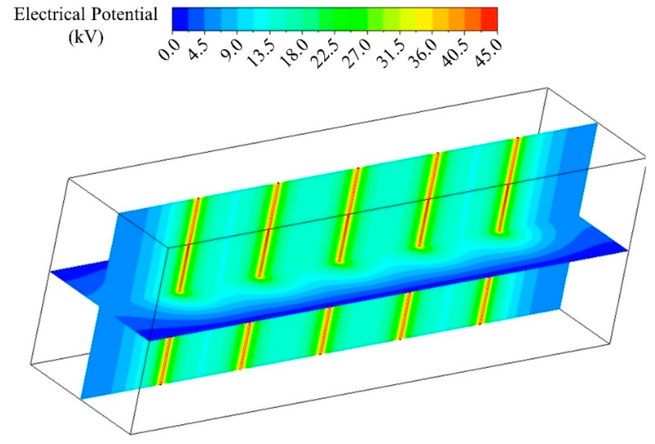
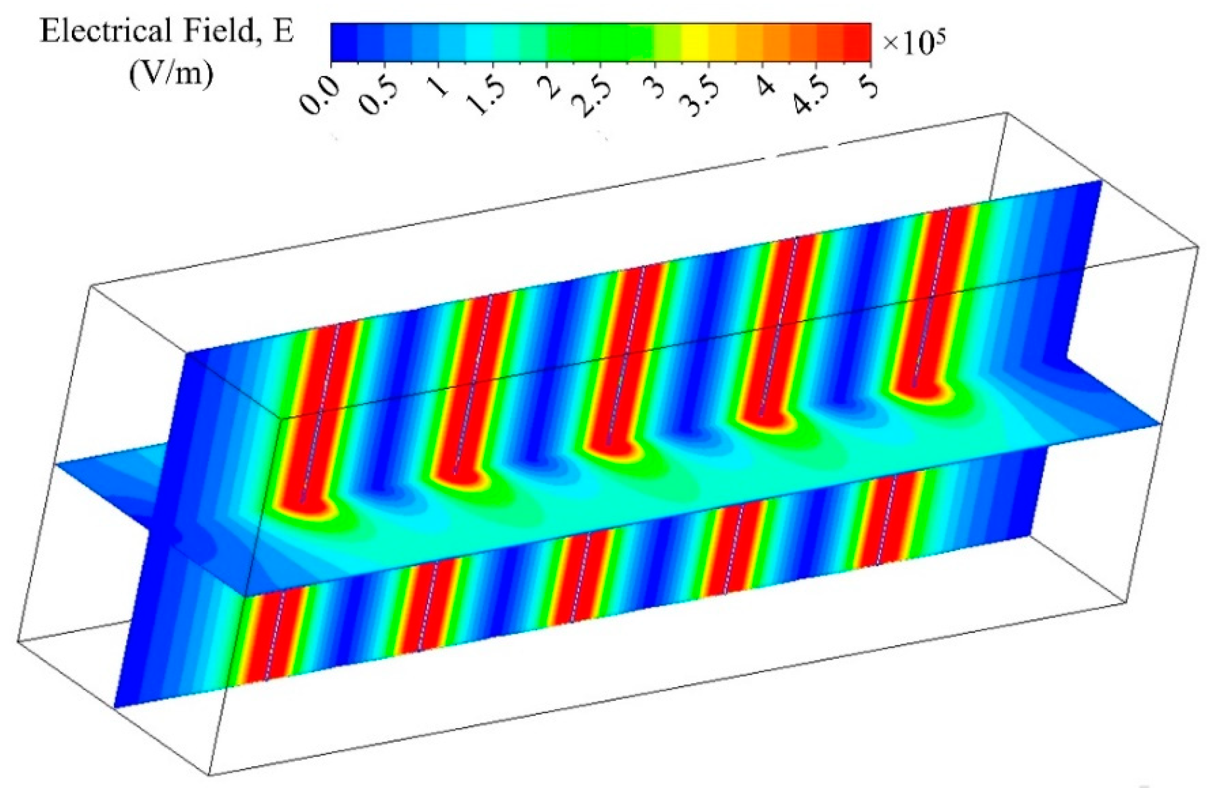
The simulated velocity distribution for the 1 m/s inlet velocity is shown in Figure 6a,b. While the velocity is almost homogeny in the flow zone of the channel, boundary layers develop over the solid wall. Down stream flow structure is affected by the existence of the corona wires. Although there are strong velocity gradients at down stream of the wire regions, these have no significant effects on the bulk flow. The calculated electric potential, current density distribution, and electric field distributions for the case of dw = 1 mm, 45 kV, and 2 m/s in 230 mm wide channel are given in Figure 7, Figure 8 and Figure 9, respectively. It is seen from the figures that the electric potential, electric field, and current density values have a maximum value at the vicinity of discharge wires, and their magnitude sharply decreases towards the collection plate electrodes at which the voltage is set as zero or grounded. As a result, particles that are placed within proximity of the wire electrodes are more strongly (rapidly) charged due to the high electric field and current density vicinity of the corona wire electrodes.
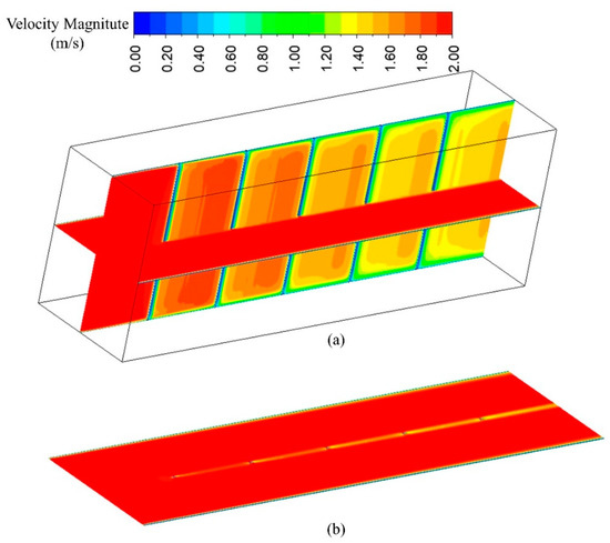
Figure 6.
Velocity magnitude distribution at the midplanes (a) and the solo view at the horizontal plane (b) for the case of dw = 1 mm, 45 kV, and Uin = 2 m/s in the 230 mm wide channel.

Figure 7.
Distribution of electric potential values at the midplanes in the case of dw = 1 mm, 45 kV, and Uin = 2 m/s in the 230 mm wide channel.
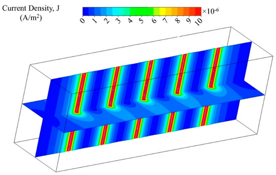
Figure 8.
Distribution of current density (J) magnitude at the midplanes in the case of dw = 1 mm, 45 kV, and Uin = 2 m/s in the 230 mm wide channel.
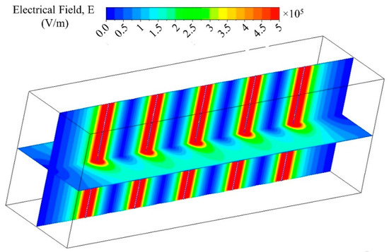
Figure 9.
Distribution of electric field (E) magnitude at the midplanes in the case of dw = 1 mm, 45 kV, and Uin = 2 m/s in the 230 mm wide channel.
Particles are injected into the computational domain from the inlet surface, and the motions and charging process of particles were calculated once through the domain. Collection efficiency as a function of the particle diameter can be obtained by using Equation (23). Figure 10 shows the particle tracking pathlines with respect to residence time for the case of 1 mm wire diameter, 55 kV, and Uin = 1 m/s in the 230 mm wide channel. It can be seen that when particle diameters are large, most of the particles are trapped close to the inlet in a very short residence time. However, residence time increases with decreasing particle diameter, and particles may travel along the ESP channel. On the other hand, the nano-size particles such as dp = 0.02 µm have smaller residence time than the one micrometre (dp = 1 µm) particles.
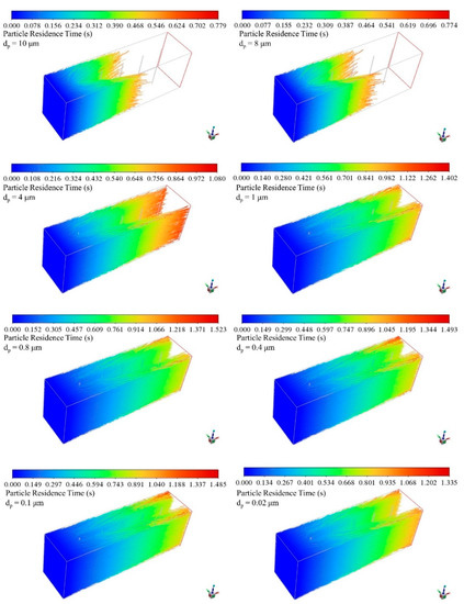
Figure 10.
Particle tracking pathlines with respect to residence time for the case of dw = 1 mm, 55 kV, and Uin = 1 m/s in the 230 mm wide channel.
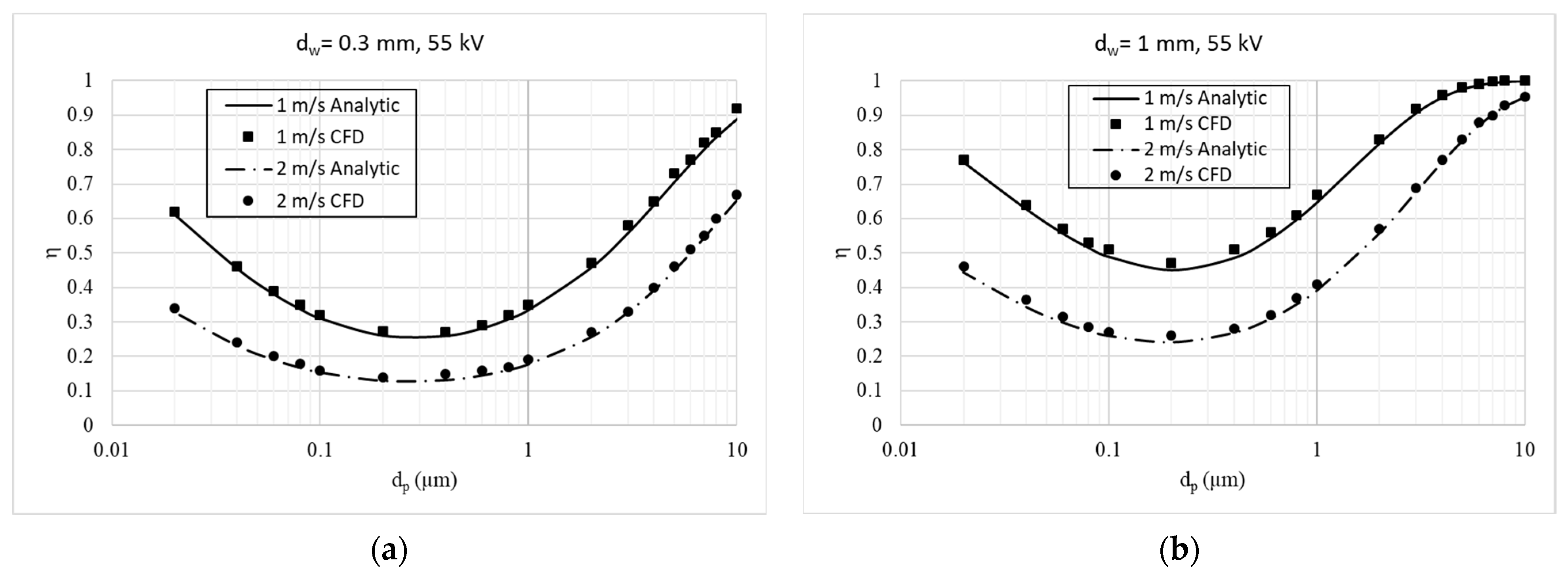
Figure 11 shows the comparison of collection efficiency values obtained with analytic and CFD models for Sy = 115 mm, applied potential 55 kV, and corona wire diameters dw = 0.3 mm and dw = 1 mm. It can be seen that the present numerical and the analytic models have a good agreement. The discrepancies are less than 10 percent for all particle diameters range. It is noted that the horizontal axis is given on a logarithmic scale. It can be seen that a higher corona wire diameter results in better collection efficiencies compared to a smaller diameter one. In addition to that, the inlet velocity significantly affects the efficiency. Smaller velocity (Uin = 1 m/s) results in better efficiency values than a higher one (Uin = 2 m/s) for all cases. It can be said that the analytic model can be used confidently for further evaluations of the collection efficiencies for the wire-plate type ESPs.

Figure 11.
Comparison of collection efficiency values obtained analytic and CFD models for Sy = 115 mm, applied potential 55 kV, corona wire diameters: (a) dw = 0.3 mm, (b) dw = 1 mm.
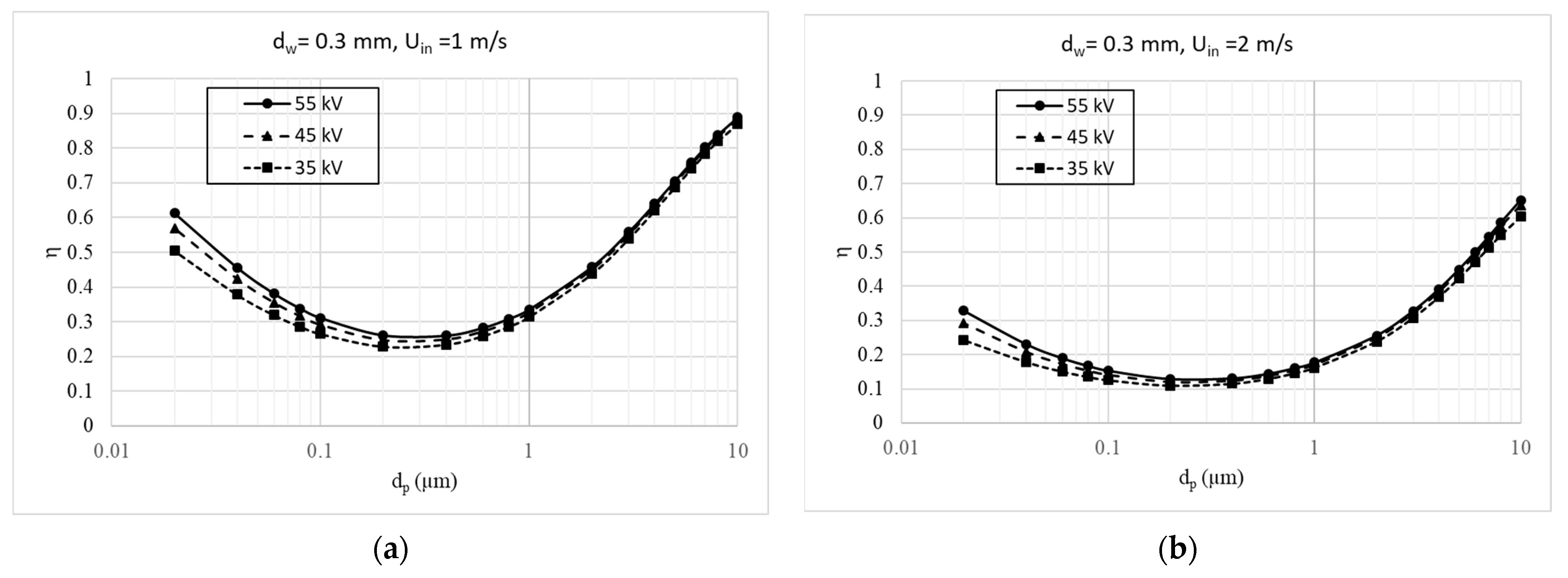
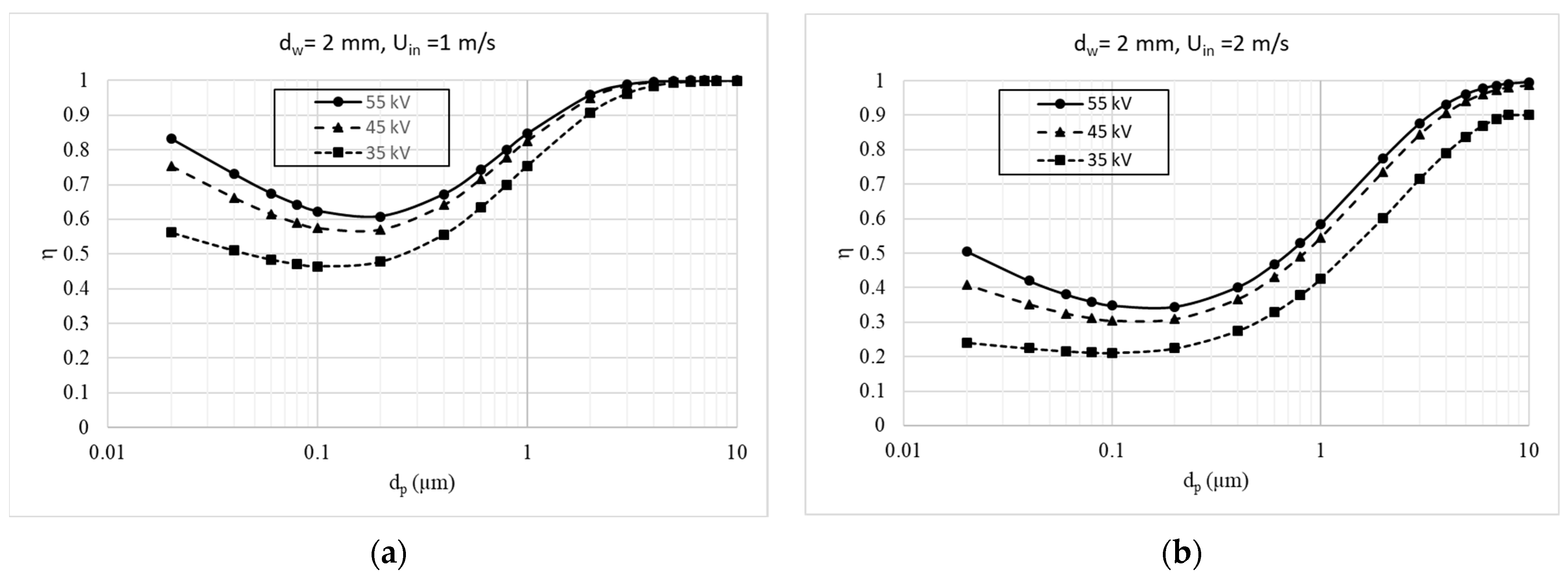
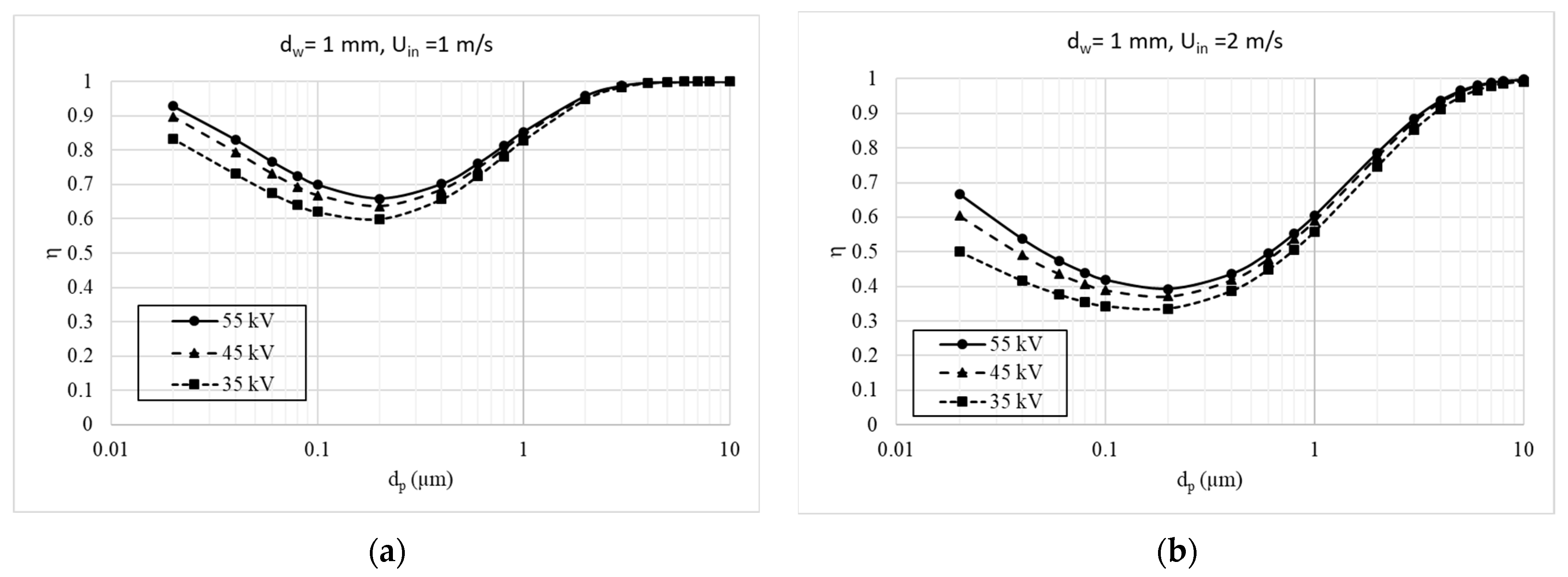
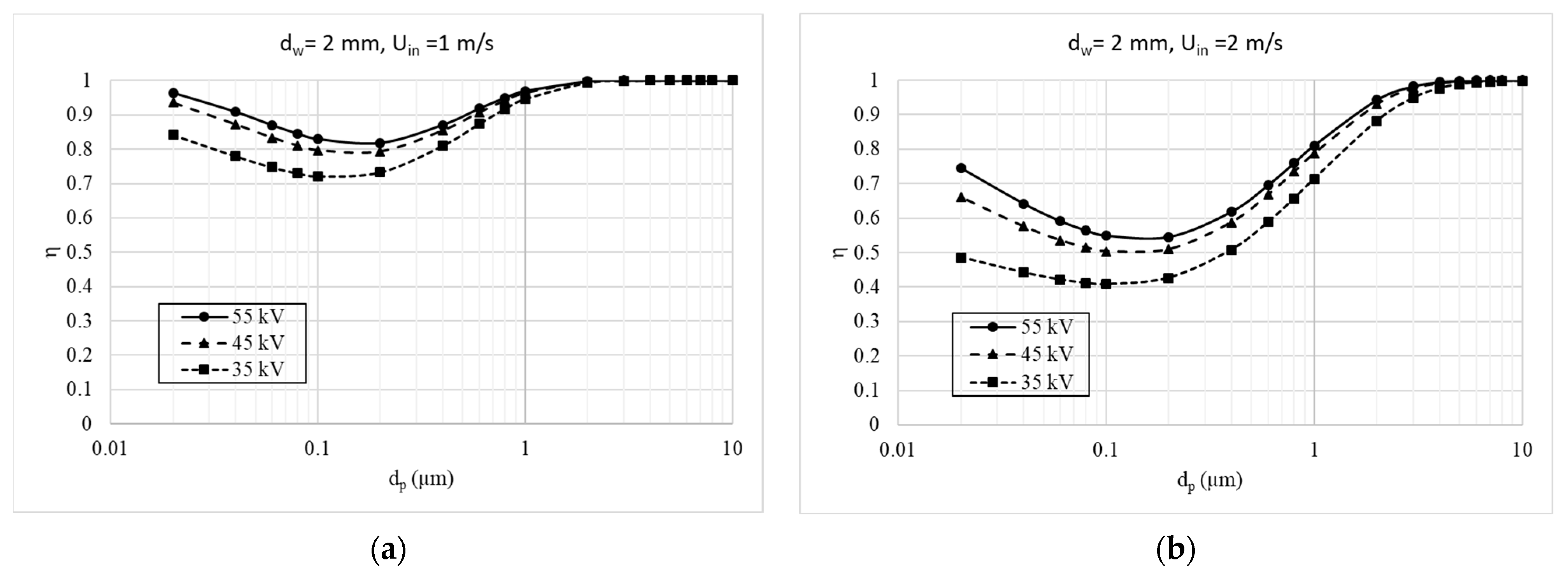
Figure 12, Figure 13 and Figure 14 show the calculated collection efficiency variation with the particle diameters for different operating conditions in the 23 cm width channels by using dw = 0.3 mm, 1 mm, and 2 mm corona wire diameters, respectively. Comparing Figure 12, Figure 13 and Figure 14, it can be observed that the corona wire electrode diameter significantly affects the collection efficiency; larger wire diameters result in better efficiency values for all ranges of particle diameters in all considered cases. It can be clearly seen that increasing the potential value significantly increase the collection efficiencies, whereas increasing the inlet velocity magnitude significantly decreases the collection efficiencies for all the considered ranges of particles. Smaller velocity (Uin = 1 m/s) results in better efficiency values than a higher one (Uin = 2 m/s) for all cases.
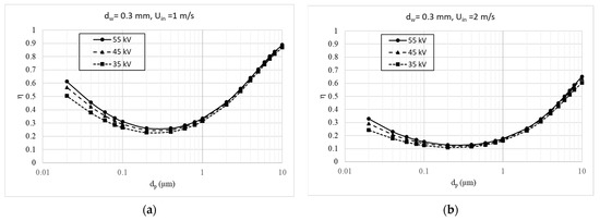
Figure 12.
Variation of the ESP collection efficiency with particle diameter for Sy = 115 mm, dw = 0.3 mm, (a) Uin = 1 m/s, (b) Uin = 2 m/s.
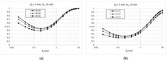
Figure 13.
Variation of the ESP collection efficiency with particle diameter for Sy = 115 mm, dw = 1 mm, (a) Uin = 1 m/s, (b) Uin = 2 m/s.

Figure 14.
Variation of the ESP collection efficiency with particle diameter for Sy = 115 mm, dw = 2 mm, (a) Uin = 1 m/s, (b) Uin = 2 m/s.
Collection efficiencies generally have a minimum of about 0.1–0.2 µm particle size for all cases. This minimum efficiency particle size is also named as the most penetrating particle size (MPPS). Although the collection efficiency values change with the operating conditions, the range of most penetrating particle sizes (MPPS) stays almost constant. This results from the increase of diffusion charging for smaller size (dp ≤ 1 µm) particles. It should be mentioned that the collection efficiencies for the particle diameters less than 3 µm are relatively quite low than the ones for the larger particles for all the cases considered in this study. Remarkably better performance was shown by 55 kV potential cases for all the particle diameter range and the cases considered.
Figure 15, Figure 16 and Figure 17 show the calculated collection efficiency variation with the particle diameters for different operating conditions in the 180 mm width channels by using dw = 0.3 mm, 1 mm, and 2 mm corona wire diameters, respectively. Similar observations for the cases of 230 mm width channels are obtained. On the other hand, comparing the results of 180 and 230 mm width channel cases, it can be seen that the distance between the wire and the plate electrodes significantly affects the collection efficiency; smaller distance between the electrodes results in better efficiency values for all ranges of particle diameter. In both channel geometry, it can be clearly seen that increasing the potential value significantly increase the collection efficiencies, whereas increasing the inlet velocity magnitude significantly decreases the collection efficiencies for all the considered ranges of particles. It should be mentioned that the collection efficiencies for the particle diameters less than 3 µm are relatively quite low than the ones for the larger particles for all the cases considered in this study. Remarkably better performance was shown by 55 kV potential cases for all the particle diameter range and the cases considered. It can be concluded that a better collection efficiency can be obtained by increasing the potential difference, decreasing the gas flow velocity, and reducing the distance between the charging and collecting electrodes. It should be considered in the design of ESP the limitations of plasma generation and the particle properties.
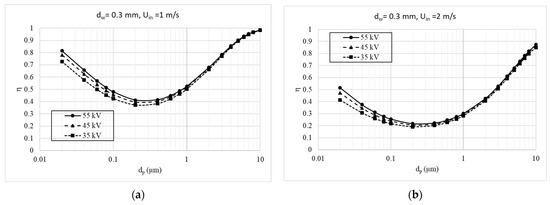
Figure 15.
Variation of the ESP collection efficiency with particle diameter for Sy = 90 mm, dw = 0.3 mm, (a) Uin = 1 m/s, (b) Uin = 2 m/s.

Figure 16.
Variation of the ESP collection efficiency with particle diameter for Sy = 90 mm, dw = 1 mm, (a) Uin = 1 m/s, (b) Uin = 2 m/s.
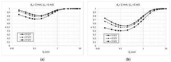
Figure 17.
Variation of the ESP collection efficiency with particle diameter for Sy = 90 mm, dw = 2 mm, (a) Uin = 1 m/s, (b) Uin = 2 m/s.
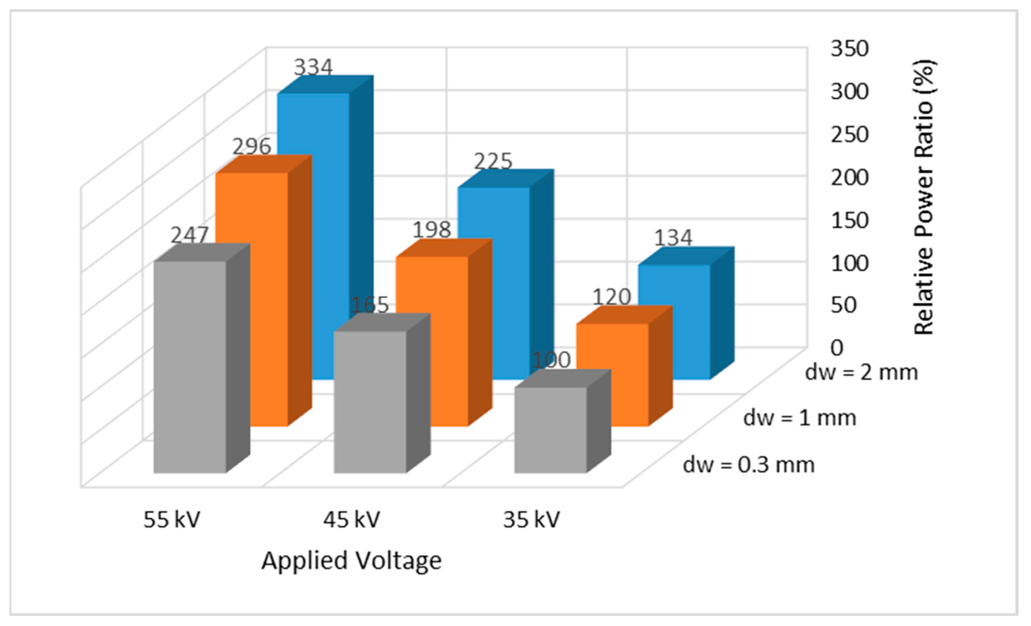
Power consumption of the ESP can be calculated as follow:
In Equation (38), P (W) is the consumed power, Δϕ (V) represents the potential difference between the electrodes, I (A) is the current observed at the collection plates. Figure 18 shows the relative power ratio variation with the corona wire diameters and the applied source voltages. It can be seen that the power consumptions of ESPs have relatively higher values with rising the applied source voltage and the corona wire diameter. Relative power consumptions of ESP with the corona wire diameters of 1 mm and 2 mm for the same source voltage are about 20 and 35 percent higher than the corona wire diameters of 0.3 mm, respectively.
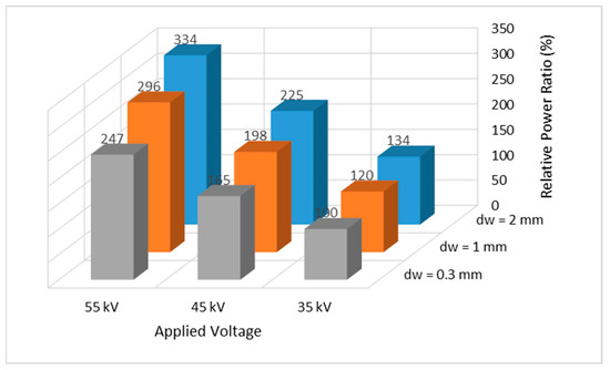
Figure 18.
Relative power consumption comparisons based on the corona wire diameter and the applied voltage.
4. Conclusions
A three-dimensional CFD model incorporating particle transport and electro-hydrodynamics in an electrostatic precipitator is constructed to investigate the flow field and the characteristics of the electrostatic field in the ESP. The present CFD model is validated with the experimental data, and the current results show very good agreement with the available experimental data. The 3D CFD model presented in this study could be used for design and detailed analysis of the ESP considering geometric, electrostatic, and particle transport parameters. In addition to that, an improved analytical model was proposed to calculate the collection efficiencies for the wire-plate type electrostatic precipitator. In all cases considered in this study, a stable fluid flow exists in the ESP channel. The main conclusions could be given as follows:
- With the decrease in the wire-plate distance, the electric field strength and the current density between the corona electrodes tends to increase. It is shown that increasing the potential difference, decreasing the gas flow velocity, and reducing the distance between the charging and collecting electrodes results in better collection efficiencies.
- Corona charge wire electrode diameter has a strong effect on the collection efficiencies. Collection efficiencies for all particle diameters are increasing with larger wire diameters. However, the energy usage of ESP increases with rising wire diameter.
- Collection efficiencies generally have a minimum of about 0.1–0.2 µm particle size for all cases. Although the collection efficiency values change with the operating conditions, the most penetrating particle size (MPPS) appears between 0.1 and 0.2 µm. This is resulted from the increase of diffusion charging effect for smaller size particles.
- The improved analytical model could be confidently used for the collection efficiency estimation of the wire-plate type ESPs.
Author Contributions
Conceptualization, M.K., M.M. and A.F.A.; Data curation, M.K., M.M. and A.F.A.; Formal analysis, M.K. and M.M.; Investigation, M.K., M.M. and A.F.A.; Methodology, M.K., M.M. and A.F.A.; Project administration, M.K.; Supervision, M.K.; Writing—original draft, M.K., M.M. and A.F.A.; Writing—review & editing, M.K., M.M. and A.F.A. All authors have read and agreed to the published version of the manuscript.
Funding
This study is supported by the Scientific and Technology Research Council of Turkey (TÜBİTAK), under project number 218M604. The authors would like to thank TÜBİTAK for his support.
Institutional Review Board Statement
Not applicable.
Informed Consent Statement
Not applicable.
Conflicts of Interest
The authors declare no conflict of interest.
References
- Tsai, C.-J.; Pui, D.Y.; Editorial, H. Recent advances and new challenges of occupational and environmental health of nanotechnology. J. Nanoparticle Res. 2009, 11, 1–4. [Google Scholar] [CrossRef]
- Tsai, C.-J.; Wu, C.-H.; Leu, M.L.; Chen, S.-C.; Huang, C.Y.; Tsai, P.C.; Ko, F.-H. Dustiness test of nanopowders using a standard rotating drum with a modified sampling train. J. Nanoparticle Res. 2009, 11, 121–131. [Google Scholar] [CrossRef]
- Tsai, C.-J.; Huang, C.-Y.; Chen, S.-C.; Ho, C.-E.; Huang, C.-H.; Chen, C.-W.; Chang, C.-P.; Tsai, S.-J.; Ellenbecker, M.J. Exposure assessment of nano-sized and respirable particles at different workplaces. J. Nanoparticle Res. 2011, 13, 4161–4172. [Google Scholar] [CrossRef]
- Bango, J.J.; Agostinelli, S.A.; Maroney, M.; Dziekan, M.; Deeb, R.; Duman, G. A Pandemic Early Warning System Decision Analysis Concept Utilizing a Distributed Network of Air Samplers via Electrostatic Air Precipitation. Appl. Sci. 2021, 11, 5308. [Google Scholar] [CrossRef]
- Altun, A.F.; Kilic, M. Utilization of electrostatic precipitators for healthy indoor environments. E3S Web Conf. 2019, 111, 02020. [Google Scholar] [CrossRef] [Green Version]
- Lin, G.-Y.; Tsai, C.-J. Numerical Modeling of Nanoparticle Collection Efficiency of Single-Stage Wire-in-Plate Electrostatic Precipitators. Aerosol Sci. Technol. 2010, 44, 1122–1130. [Google Scholar] [CrossRef] [Green Version]
- Trnka, J.; Jandačka, J.; Holubčík, M. Improvement of the Standard Chimney Electrostatic Precipitator by Dividing the Flue Gas Stream into a Larger Number of Pipes. Appl. Sci. 2022, 12, 2659. [Google Scholar] [CrossRef]
- Wang, W.; Yang, L.; Wu, K.; Lin, C.; Huo, P.; Liu, S.; Huang, D.; Lin, M. Regulation-controlling of boundary layer by multi-wire-to-cylinder negative corona discharge. Appl. Therm. Eng. 2017, 119, 438–448. [Google Scholar] [CrossRef]
- Lu, Q.; Yang, Z.; Zheng, C.; Li, X.; Zhao, C.; Xu, X.; Gao, X.; Luo, Z.; Ni, M.; Cen, K. Numerical simulation on the fine particle charging and transport behaviors in a wire-plate electrostatic precipitator. Adv. Powder Technol. 2016, 27, 1905–1911. [Google Scholar] [CrossRef]
- Dong, M.; Zhou, F.; Zhang, Y.; Shang, Y.; Li, S. Numerical study on fine-particle charging and transport behaviour in electrostatic precipitators. Powder Technol. 2018, 330, 210–218. [Google Scholar] [CrossRef]
- He, M.; Luo, Z.; Wang, H.; Fang, M. The Influences of Acoustic and Pulsed Corona Discharge Coupling Field on Agglomeration of Monodisperse Fine Particles. Appl. Sci. 2020, 10, 1045. [Google Scholar] [CrossRef] [Green Version]
- Guo, B.; Yu, A.; Guo, J. Numerical Modelling of electrostatic precipitation: Effect of Gas temperature. J. Aerosol Sci. 2014, 77, 102–115. [Google Scholar] [CrossRef]
- Adamiak, K. Numerical models in simulating wire-plate electrostatic precipitators: A review. J. Electrostat. 2013, 71, 673–680. [Google Scholar] [CrossRef]
- Arif, S.; Branken, D.J.; Everson, R.C.; Neomagus, H.W.J.P.; le Grange, L.A.; Arif, A. CFD modeling of particle charging and collection in electrostatic precipitators. J. Electrostat. 2016, 84, 10–22. [Google Scholar] [CrossRef]
- Haque, S.; Rasul, M.; Deev, A.; Khan, M.M.; Subaschandar, N. Flow simulation in an electrostatic precipitator of a thermal power plant. Appl. Therm. Eng. 2009, 29, 2037–2042. [Google Scholar] [CrossRef]
- Choi, B.S.; Fletcher, C.A.J. Computation of particle transport in an electrostatic precipitator. J. Electrostat. 1997, 40–41, 413–418. [Google Scholar] [CrossRef]
- Adamiak, K. Simulation of corona in wire-duct electrostatic precipitator by means of the boundary element method. IEEE Trans. Ind. Appl. 1994, 30, 381–386. [Google Scholar] [CrossRef]
- Khaled, U.; El Dein, A. Experimental study of V–I characteristics of wire–plate electrostatic precipitators under clean air conditions. J. Electrostat. 2013, 71, 228–234. [Google Scholar] [CrossRef]
- Anagnostopoulos, J.; Bergeles, G. Corona discharge simulation in wire-duct electrostatic precipitator. J. Electrost. 2002, 54, 129–147. [Google Scholar] [CrossRef]
- Zhang, X.; Lianze, W.; Keqin, Z. An analysis of a wire-plate electrostatic precipitator. J. Aerosol Sci. 2002, 33, 1595–1600. [Google Scholar] [CrossRef]
- Zhang, X.; Wang, L.; Zhu, K. Particle tracking and particle-wall collision in a wire-plate electrostatic precipitator. J. Electrost. 2005, 63, 1057–1071. [Google Scholar] [CrossRef]
- Cooperman, P. A new theory of precipitator efficiency. Atmos. Environ. 1971, 5, 541–551. [Google Scholar] [CrossRef]
- Yang, Z.; Li, H.; Li, Q.; Lin, R.; Jiang, Y.; Yang, Y.; Zheng, C.; Sun, D.; Gao, X. Correlations between Particle Collection Behaviors and Electrohydrodynamics Flow Characteristics in Electrostatic Precipitators. Aerosol Air Qual. Res. 2020, 20, 2901–2910. [Google Scholar] [CrossRef]
- Wen, T.-Y.; Krichtafovitch, I.; Mamishev, A.V. Numerical study of electrostatic precipitators with novel particle-trapping mechanism. J. Aerosol Sci. 2016, 95, 95–103. [Google Scholar] [CrossRef]
- Park, J.W.; Kim, C.; Park, J.; Hwang, J. Computational fluid dynamic modelling of particle charging and collection in a wire-to-plate type single-stage electrostatic precipitator. Aerosol Air Qual. Res. 2018, 18, 590–601. [Google Scholar] [CrossRef] [Green Version]
- Tu, G.; Song, Q.; Yao, Q. Experimental and numerical study of particle deposition on perforated plates in a hybrid electrostatic filter precipitator. Powder Technol. 2017, 321, 143–153. [Google Scholar] [CrossRef]
- Kilic, M.; Sevilgen, G. Modelling airflow, heat transfer and moisture transport around a standing human body by computational fluid dynamics. Int. Commun. Heat Mass Transf. 2008, 35, 1159–1164. [Google Scholar] [CrossRef]
- Sevilgen, G.; Kılıç, M. Numerical analysis of air flow, heat transfer, moisture transport and thermal comfort in a room heated by two-panel radiators. Energy Build. 2011, 43, 137–146. [Google Scholar] [CrossRef]
- ANSYS. Ansys Fluent 19.0 Theory Guide; Release 19.0; ANSYS Inc.: Canonsburg, PA, USA, 2021. [Google Scholar]
- Allen, M.D.; Raabe, O.G. Re-evaluation of millikan’s oil drop data for the motion of small particles in air. J. Aerosol Sci. 1982, 13, 537–547. [Google Scholar] [CrossRef]
- Hinds, W.C. Aerosol Technology, 2nd ed.; John Wiley & Sons: New York, NY, USA, 1999. [Google Scholar]
- Lawless, P.A. Particle charging bounds, symmetry relations, and an analytic charging rate model for the continuum regime. J. Aerosol Sci. 1996, 27, 191–215. [Google Scholar] [CrossRef]
- Kılıç, M.; Mutlu, İ.H.; Saldamlı, I. Numerical investigation of an air cleaning device performance. J. Fac. Eng. Arch. Gazi Univ. 2022, 37, 2077–2089. [Google Scholar] [CrossRef]
- Penny, G.W.; Matick, R.E. Potentials in D-C corona fields. Trans. AIEE Part I Comm. Electron. 1960, 79, 91–99. [Google Scholar] [CrossRef]
- Kihm, K.D. Effects of Nonuniformities on Particle Transport in Electrostatic Precipitators. Ph.D. Thesis, Department of Mechanical Engineering, Stanford University, Stanford, CA, USA, 1987. [Google Scholar]
- Deutsch, W. Bewegung und Ladung der Elektrizitätsträger im Zylinderkondensator. Ann. Phys. 1922, 373, 335–344. [Google Scholar] [CrossRef] [Green Version]
- Leonard, G.; Mitchner, M.; Self, S.A. Particle transport in electrostatic precipitators. Atmos. Environ. 1980, 14, 1289–1299. [Google Scholar] [CrossRef]
- Leonard, G.L.; Mitchner, M.; Self, S.A. An experimental study of the electrohydrodynamic flow in electrostatic precipitators. J. Fluid Mech. 1983, 127, 123–140. [Google Scholar] [CrossRef]
- Leonard, G.L.; Mitchner, M.; Self, S.A. Experimental study of the effect of turbulent diffusion on precipitator efficiency. J. Aerosol Sci. 1982, 13, 271–284. [Google Scholar] [CrossRef]
- Kim, S.H.; Lee, K.W. Experimental study of electrostatic precipitator performance and comparison with existing theoretical prediction models. J. Electrostat. 1999, 48, 3–25. [Google Scholar] [CrossRef]
- Lin, G.-Y.; Chen, T.-M.; Tsai, C.-J. A Modified Deutsch-Anderson Equation for Predicting the Nanoparticle Collection Efficiency of Electrostatic Precipitators. Aerosol Air Qual. Res. 2012, 12, 697–706. [Google Scholar] [CrossRef]
- Yuan, C.S.; Shen, T.T. Electrostatic Precipitation. In Air Pollution Control Engineering; Wang, L.K., Pereira, N.C., Hung, Y.T., Eds.; Humana Press Inc.: Totowa, NJ, USA, 2004; pp. 172–196. [Google Scholar]
- Yoo, K.H.; Lee, J.S.; Oh, M. Do Charging and Collection of Submicron Particles in Two-Stage Parallel-Plate Electrostatic Precipitators. Aerosol Sci. Technol. 1997, 27, 308–323. [Google Scholar] [CrossRef] [Green Version]
- Kim, S.H.; Park, H.S.; Lee, K.W. Theoretical model of electrostatic precipitator performance for collecting polydisperse particles. J. Electrostat. 2001, 50, 177–190. [Google Scholar] [CrossRef]
- Park, J.-H.; Chun, C.-H. An improved modelling for prediction of grade efficiency of electrostatic precipitators with negative corona. J. Aerosol Sci. 2002, 33, 673–694. [Google Scholar] [CrossRef]
- McDonald, J.R.; Smith, W.B.; Spencer, H.W., III; Sparks, L.E. A mathematical model for calculating electrical conditions in wire-duct electrostatic precipitation devices. J. Appl. Phys. 1977, 48, 2231–2243. [Google Scholar] [CrossRef]


Publisher’s Note: MDPI stays neutral with regard to jurisdictional claims in published maps and institutional affiliations. |
© 2022 by the authors. Licensee MDPI, Basel, Switzerland. This article is an open access article distributed under the terms and conditions of the Creative Commons Attribution (CC BY) license (https://creativecommons.org/licenses/by/4.0/).