Figure 1.
The prototype and model of the controllable mechanism welding robot.
Figure 1.
The prototype and model of the controllable mechanism welding robot.
Figure 2.
Experimental system for verification.
Figure 2.
Experimental system for verification.
Figure 3.
(a) First-order simulation mode diagram; (b) First-order test mode diagram.
Figure 3.
(a) First-order simulation mode diagram; (b) First-order test mode diagram.
Figure 4.
(a) Second-order simulation mode diagram; (b) Second-order test mode diagram.
Figure 4.
(a) Second-order simulation mode diagram; (b) Second-order test mode diagram.
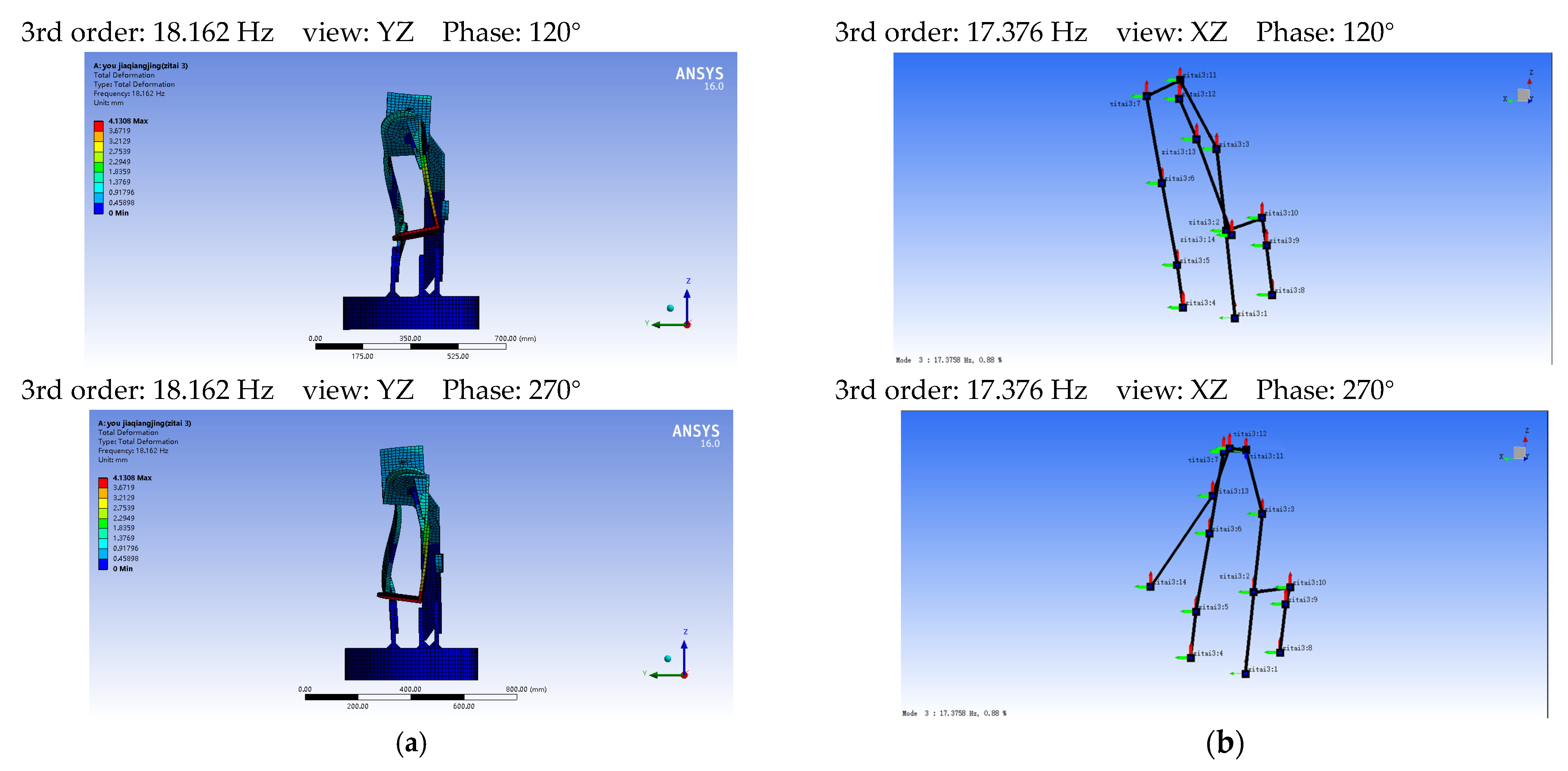
Figure 5.
(a) Third-order simulation mode diagram; (b) Third-order test mode diagram.
Figure 5.
(a) Third-order simulation mode diagram; (b) Third-order test mode diagram.
Figure 6.
(a) Fourth-order simulation mode diagram; (b) Fourth-order test mode diagram.
Figure 6.
(a) Fourth-order simulation mode diagram; (b) Fourth-order test mode diagram.
Figure 7.
Central composite design (CCD) and Box-Behnken design (BBD).
Figure 7.
Central composite design (CCD) and Box-Behnken design (BBD).
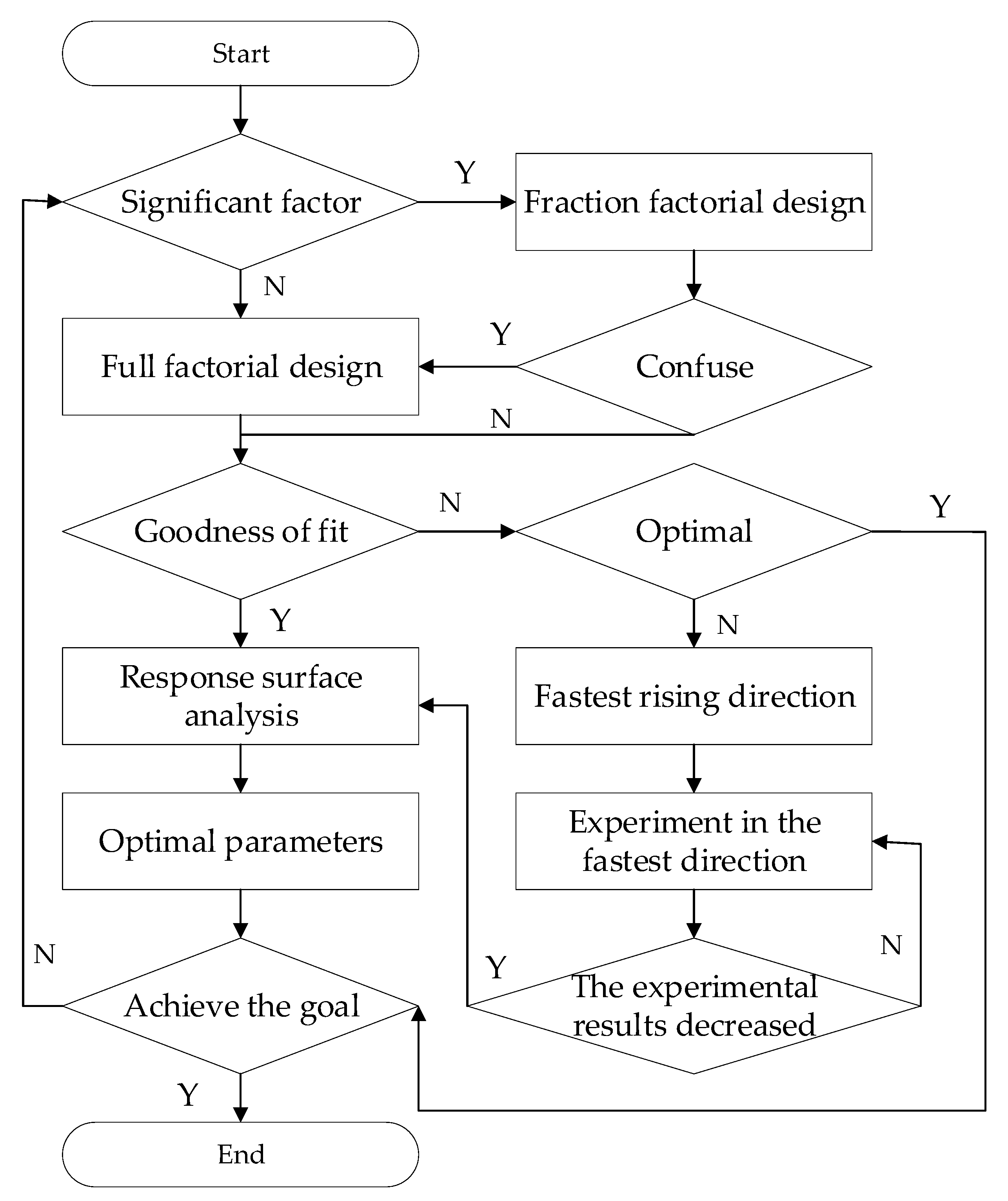
Figure 8.
General flow of experimental design.
Figure 8.
General flow of experimental design.
Figure 9.
The distribution of excitation sources.
Figure 9.
The distribution of excitation sources.
Figure 10.
Series-parallel controllable mechanism welding robot component names.
Figure 10.
Series-parallel controllable mechanism welding robot component names.
Figure 11.
Main effect diagrams of maximum amplitude displacement at the end of a series-parallel controllable mechanisms welding robot.
Figure 11.
Main effect diagrams of maximum amplitude displacement at the end of a series-parallel controllable mechanisms welding robot.
Figure 12.
Interaction diagrams of the maximum amplitude displacement at the end of a series-parallel controllable mechanism welding robot (The sign * in the figure means the interaction of two factors).
Figure 12.
Interaction diagrams of the maximum amplitude displacement at the end of a series-parallel controllable mechanism welding robot (The sign * in the figure means the interaction of two factors).
Figure 13.
Response optimizer optimization diagram of excitation design.
Figure 13.
Response optimizer optimization diagram of excitation design.
Figure 14.
Amplitude response curve of the terminal surface after excitation optimization.
Figure 14.
Amplitude response curve of the terminal surface after excitation optimization.
Figure 15.
Main effect diagrams for the maximum amplitude displacement at the end of welding robot: (a) 16 Hz;(b) 18 Hz; (c) 24 Hz; (d) 25 Hz; (e) 45 Hz.
Figure 15.
Main effect diagrams for the maximum amplitude displacement at the end of welding robot: (a) 16 Hz;(b) 18 Hz; (c) 24 Hz; (d) 25 Hz; (e) 45 Hz.
Figure 16.
Interaction diagrams for the amplitude displacement at the end of the welding robot: (a) 16 Hz; (b) 18 Hz; (c) 24 Hz; (d) 25 Hz; (e) 45 Hz. (The sign * in the figure means the interaction of two factors).
Figure 16.
Interaction diagrams for the amplitude displacement at the end of the welding robot: (a) 16 Hz; (b) 18 Hz; (c) 24 Hz; (d) 25 Hz; (e) 45 Hz. (The sign * in the figure means the interaction of two factors).
Figure 17.
Optimization diagram of bar thickness design.
Figure 17.
Optimization diagram of bar thickness design.
Figure 18.
Amplitude response curve of the terminal surface after the optimization of the bar thickness.
Figure 18.
Amplitude response curve of the terminal surface after the optimization of the bar thickness.
Figure 19.
The main effect diagrams of the maximum displacement at the end: (a) 16 Hz; (b) 18 Hz.
Figure 19.
The main effect diagrams of the maximum displacement at the end: (a) 16 Hz; (b) 18 Hz.
Figure 20.
Interaction diagrams of the amplitude displacement at the end of the welding robot: (a) 16 Hz; (b) 18 Hz. (The sign * in the figure means the interaction of two factors).
Figure 20.
Interaction diagrams of the amplitude displacement at the end of the welding robot: (a) 16 Hz; (b) 18 Hz. (The sign * in the figure means the interaction of two factors).
Figure 21.
Optimization diagram of member damping design.
Figure 21.
Optimization diagram of member damping design.
Figure 22.
Optimization diagrams of coupling effects design.
Figure 22.
Optimization diagrams of coupling effects design.
Figure 23.
Amplitude response curve of the terminal surface after comprehensive optimization.
Figure 23.
Amplitude response curve of the terminal surface after comprehensive optimization.
Table 1.
Comparison of the first seven natural frequencies between the simulations and tests.
Table 1.
Comparison of the first seven natural frequencies between the simulations and tests.
| Order | Simulation Result (Hz) | Experimental Result (Hz) | Error Rate |
|---|
| 1 | 10.27 | 9.415 | 9.081% |
| 2 | 15.917 | 16.504 | 3.557% |
| 3 | 18.162 | 17.376 | 4.523% |
| 4 | 37.23 | 37.105 | 0.337% |
| 5 | 46.456 | 42.683 | 8.840% |
| 6 | 54.059 | 52.658 | 2.661% |
| 7 | 80.016 | 83.801 | 4.517% |
Table 2.
Center composite design experimental data design of excitation sources.
Table 2.
Center composite design experimental data design of excitation sources.
| Order | Moment (N∙mm) | Order | Moment (N∙mm) |
|---|
| 1 | 2 | 3 | 4 | 5 | 1 | 2 | 3 | 4 | 5 |
|---|
| 1 | 2200 | 2600 | 1100 | 620 | 300 | 18 | 2400 | 2000 | 900 | 640 | 320 |
| 2 | 2200 | 2200 | 1100 | 620 | 340 | 19 | 2000 | 2000 | 1300 | 640 | 320 |
| 3 | 2200 | 2200 | 1100 | 660 | 300 | 20 | 2000 | 2400 | 900 | 600 | 280 |
| 4 | 1800 | 2200 | 1100 | 620 | 300 | 21 | 2000 | 2400 | 1300 | 640 | 280 |
| 5 | 2200 | 2200 | 1100 | 580 | 300 | 22 | 2200 | 2200 | 1100 | 620 | 300 |
| 6 | 2600 | 2200 | 1100 | 620 | 300 | 23 | 2400 | 2400 | 900 | 640 | 280 |
| 7 | 2200 | 2200 | 1100 | 620 | 260 | 24 | 2000 | 2400 | 1300 | 600 | 320 |
| 8 | 2200 | 2200 | 700 | 620 | 300 | 25 | 2000 | 2400 | 900 | 640 | 320 |
| 9 | 2200 | 2200 | 1500 | 620 | 300 | 26 | 2400 | 2400 | 1300 | 600 | 280 |
| 10 | 2200 | 1800 | 1100 | 620 | 300 | 27 | 2200 | 2200 | 1100 | 620 | 300 |
| 11 | 2200 | 2200 | 1100 | 620 | 300 | 28 | 2200 | 2200 | 1100 | 620 | 300 |
| 12 | 2000 | 2000 | 1300 | 600 | 280 | 29 | 2000 | 2000 | 900 | 640 | 280 |
| 13 | 2400 | 2000 | 1300 | 640 | 280 | 30 | 2400 | 2400 | 900 | 600 | 320 |
| 14 | 2200 | 2200 | 1100 | 620 | 300 | 31 | 2200 | 2200 | 1100 | 620 | 300 |
| 15 | 2400 | 2000 | 900 | 600 | 280 | 32 | 2000 | 2000 | 900 | 600 | 320 |
| 16 | 2200 | 2200 | 1100 | 620 | 300 | 33 | 2400 | 2400 | 1300 | 640 | 320 |
| 17 | 2400 | 2000 | 1300 | 600 | 320 | | | | | | |
Table 3.
Center composite design experimental data design table of bar thickness.
Table 3.
Center composite design experimental data design table of bar thickness.
| Order | Connecting Rod 2 (mm) | Swing Arm g (mm) | End g (mm) | Order | Connecting Rod 2 (mm) | Swing Arm g (mm) | End g (mm) |
|---|
| 1 | 14 | 9 | 10.633 | 11 | 12 | 8 | 8 |
| 2 | 14 | 9 | 9 | 12 | 12 | 8 | 10 |
| 3 | 14 | 7.367 | 9 | 13 | 12 | 9 | 9 |
| 4 | 14 | 9 | 7.367 | 14 | 14 | 9 | 9 |
| 5 | 14 | 9 | 9 | 15 | 16 | 10 | 10 |
| 6 | 17.266 | 9 | 9 | 16 | 12 | 10 | 10 |
| 7 | 14 | 10.633 | 9 | 17 | 14 | 9 | 9 |
| 8 | 10.735 | 9 | 9 | 18 | 14 | 8 | 10 |
| 9 | 12 | 10 | 8 | 19 | 16 | 8 | 8 |
| 10 | 16 | 10 | 8 | 20 | 14 | 9 | 9 |
Table 4.
Center composite design experimental data design table of damping values.
Table 4.
Center composite design experimental data design table of damping values.
| Order | Driving Rod 1 | Connecting Rod 1 | End g | Order | Driving Rod 1 | Connecting Rod 1 | End g |
|---|
| 1 | 0.0020 | 0.0260 | 0.0260 | 11 | 0.0113 | 0.0407 | 0.0407 |
| 2 | 0.0260 | 0.0020 | 0.0260 | 12 | 0.0113 | 0.0113 | 0.0113 |
| 3 | 0.0260 | 0.0260 | 0.0260 | 13 | 0.0407 | 0.0407 | 0.0113 |
| 4 | 0.0260 | 0.0260 | 0.0500 | 14 | 0.0113 | 0.0407 | 0.0113 |
| 5 | 0.0260 | 0.0260 | 0.0260 | 15 | 0.0407 | 0.0113 | 0.0407 |
| 6 | 0.0260 | 0.0500 | 0.0260 | 16 | 0.0260 | 0.0260 | 0.0260 |
| 7 | 0.0500 | 0.0260 | 0.0260 | 17 | 0.0407 | 0.0113 | 0.0113 |
| 8 | 0.0260 | 0.0260 | 0.0020 | 18 | 0.0260 | 0.0260 | 0.0260 |
| 9 | 0.0113 | 0.0113 | 0.0407 | 19 | 0.0260 | 0.0260 | 0.0260 |
| 10 | 0.0407 | 0.0407 | 0.0407 | 20 | 0.0260 | 0.0260 | 0.0260 |
Table 5.
Response optimizer optimization results of excitation design.
Table 5.
Response optimizer optimization results of excitation design.
| Response | Fitting Value | Fitting Value Error | 95% Confidence Interval | 95% Prediction Interval |
|---|
| Deformation (16 Hz) | 0.2880 | 0.0191 | (0.2459, 0.3301) | (0.2266, 0.3495) |
Table 6.
Response optimizer optimization results of bar thickness design.
Table 6.
Response optimizer optimization results of bar thickness design.
| Response | Fitting Value | Fitting Value Error | 95% Confidence Interval | 95% Prediction Interval |
|---|
| Deformation (16 Hz) | 0.0003 | 0.1220 | (−0.2760, 0.2770) | (−0.4350, 0.4360) |
| Deformation (18 Hz) | 0.0155 | 0.0147 | (−0.0177, 0.0487) | (−0.0367, 0.0677) |
| Deformation (24 Hz) | 0.0013 | 0.0139 | (−0.0303, 0.0328) | (−0.0483, 0.0509) |
| Deformation (25 Hz) | 0.0876 | 0.1450 | (−0.2410, 0.4160) | (−0.4290, 0.6040) |
| Deformation (45 Hz) | 0.0102 | 0.0133 | (−0.0200, 0.0404) | (−0.0373, 0.0578) |
Table 7.
Response optimizer optimization results of member damping design.
Table 7.
Response optimizer optimization results of member damping design.
| Response | Fitting Value | Fitting Value Error | 95% Confidence Interval | 95% Prediction Interval |
|---|
| Deformation (16 Hz) | 0.0147 | 0.0433 | (−0.0833, 0.1127) | (−0.1025, 0.1319) |
| Deformation (25 Hz) | 0.0169 | 0.0164 | (−0.0203, 0.0541) | (−0.0276, 0.0614) |
Table 8.
Synthesis center composite design test data design table.
Table 8.
Synthesis center composite design test data design table.
| Order | Moment 3 (N·mm) | Thickness of End g (mm) | Damping Value of Driving Rod 1 | Order | Moment 3 (N·mm) | Thickness of End g (mm) | Damping Value of Driving Rod 1 |
|---|
| 1 | 1300 | 8 | 0.0500 | 11 | 1100 | 9 | 0.0260 |
| 2 | 1300 | 8 | 0.0020 | 12 | 1100 | 9 | 0.0260 |
| 3 | 900 | 10 | 0.0500 | 13 | 1100 | 10.633 | 0.0260 |
| 4 | 900 | 10 | 0.0020 | 14 | 773.4 | 9 | 0.0260 |
| 5 | 1100 | 9 | 0.0260 | 15 | 1100 | 9 | 0.0260 |
| 6 | 1100 | 9 | 0.0260 | 16 | 1100 | 9 | 0.0652 |
| 7 | 1300 | 10 | 0.0020 | 17 | 1100 | 9 | 0.0260 |
| 8 | 900 | 8 | 0.0500 | 18 | 1100 | 7.367 | 0.0260 |
| 9 | 900 | 8 | 0.0020 | 19 | 1426.6 | 9 | 0.0260 |
| 10 | 1300 | 10 | 0.0500 | 20 | 1100 | 9 | 0.0260 |
Table 9.
Optimization graph results of coupling effects design.
Table 9.
Optimization graph results of coupling effects design.
| Response | Fitting Value | Fitting Value Error | 95% Confidence Interval | 95% Prediction Interval |
|---|
| Deformation (16 Hz) | 0.0879 | 0.0257 | (0.0297, 0.1461) | (−0.0227, 0.1985) |
| Deformation (18 Hz) | 0.0124 | 0.0078 | (−0.00518, 0.03004) | (−0.02103, 0.04588) |
| Deformation (25 Hz) | 0.0983 | 0.0244 | (0.0430, 0.1535) | (−0.0067, 0.2032) |
| Deformation (43 Hz) | 0.0000 | 0.0119 | (−0.0270, 0.0270) | (−0.0513, 0.0513) |


