Real-Time Short-Term Voltage Stability Assessment Using Combined Temporal Convolutional Neural Network and Long Short-Term Memory Neural Network

Abstract

This research presents a new method based on a combined temporal convolutional neural network and long-short term memory neural network for the real-time assessment of short-term voltage stability to keep the electric grid in a secure state. The assessment includes both the voltage instability (stable state or unstable state) and the fault-induced delayed voltage recovery phenomenon subjected to disturbance. The trained model uses the time series post-disturbance bus voltage trajectories as the input in order to predict the stability state of the power system in a computationally efficient manner. The proposed method also utilizes a transfer learning approach that acclimates to the pre-trained model using only a few labeled samples, which assesses voltage instability under unseen network topology change conditions. Finally, the performance evaluated on the IEEE 9 Bus and New England 39 Bus test systems shows that the proposed method gives superior accuracy with higher efficacy and thus is suitable for online application.

1. Introduction

Short-term voltage stability (STVS) is one of the major constraints that must be considered in order to keep today’s power supply safe and reliable. The ability of the power system to maintain the steady equilibrium state of its bus voltage subjected to large disturbance within a short period is termed as STVS. The time frame of interest for STVS is about only a few seconds subjected to large disturbance [1]. Short-term voltage instability is caused by the dynamics of induction motor load, electronically controlled load, HVDC link power regulation, and inverter-interfaced renewable generators [2,3]. In recent times, there has been a huge interest in understanding the impact of integration of different renewable energy resources (RESs) such as photovoltaic generation (PVG) and wind turbine generation (WTG) on different aspects of power systems such as small-signal, transient, and voltage stability [4,5,6,7]. The integration of RESs affects the dynamics of power systems and has a detrimental impact on the STVS of the power system. Short-term voltage instability causes catastrophic power system outages all around the world [8,9]. The online STVS assessment and its accompanying preventive strategy are effective countermeasures against short-term voltage instability in the post-disturbance state [2]. Thus, this work focuses on earlier assessment of STVS considering the impact of RESs so that the power system operator can make a quick decision to ensure the overall stability of the power system.

The goal of the STVS assessment is to look into the dynamic voltage performance subject to large disturbance. The problems related to STVS are the fast voltage collapse, sustained low voltage without recovery, and fault-induced delayed voltage recovery (FIDVR) [10]. Furthermore, an FIDVR event many lead to the tripping of the under-voltage load-shedding devices and tripping of wind turbines due to low voltage ride-through capability in a wind-integrated system. The traditional power system model-based approach of STVS assessment using time domain simulation (TDS) increases the computational time, making it unsuitable for online application. However, the real-time data of bus voltage samples can be available at the control centers using a wide area measurement system (WAMS) and phasor measurement units (PMUs), making the real-time STVS assessment feasible [11,12]. Recently, most of the research concentrates on the traditional machine learning algorithms for online assessment of STVS assessment using the voltage samples available using PMUs [10,13,14]. These algorithms, on the other hand, neglect the spectral and temporal structure of the data, omitting some of the most important features throughout the learning process, resulting in skewed outcomes.

Deep learning algorithms have recently been used to learn high-level features from data, alleviating the need for domain expertise, and a separate feature extraction technique, which are required in a traditional machine learning approach. In addition, deep learning algorithms works well on prediction the time series data compared to machine learning algorithms [15,16]. Furthermore, deep learning algorithms such as the convolutional neural network (CNN), the long short-term memory (LSTM) neural network, and the combined graph convolutional network and long short-term memory (GCN-LSTM) have been developed to address the problem related to short-term voltage instability [17,18,19]. Apart from this, the deep learning algorithms such as a bi-directional gated recurrent unit with an attention mechanism [20] and spatial–temporal graph convolutional network (STGCN) [21] which can learn temporal features and spatial–temporal features, respectively, from the time series data are used to predict the short-term voltage instability state of the power system. However, these studies are confined to predicting the voltage instability state: stable or unstable. They continue to overlook the possibility of an FIDVR phenomena that still exists on power systems subjected to disturbance. As a result, a complete method capable of assessing both the voltage instability mode and the FIDVR phenomenon concurrently within the short observation time window (OTW) is required.

Conventionally, machine learning algorithms and deep learning algorithms for the assessment of voltage stability require the manual labeling of a large number of data samples, which is computationally expensive and time consuming [17,18,19,22,23]. When the network topology changes, most of the machine learning and deep learning algorithms fail in prediction, requiring frequent model updates with large data sets, which is time consuming and infeasible for online application [24,25]. Recently, many research studies have been conducted based on transfer learning (TL) where the same model trained to solve one particular task can be utilized to solve another but related task with few labeled samples [26,27,28,29]. However, none of the studies in the literature found so far have utilized the deep learning-based transfer learning concept for the assessment of STVS for the N-1 contingency cases using a single learning model. As a result, developing an STVS assessment approach that can acclimate to the new environment using a small set of labeled data sample is critical.

The objective of this research is to resolve the research gaps mentioned above. It is an extension of our previous study [30] which further proposes the combined temporal convolutional neural network and long short-term memory neural network for the assessment of STVS considering the impact of RESs. The following are the primary contributions of this work:

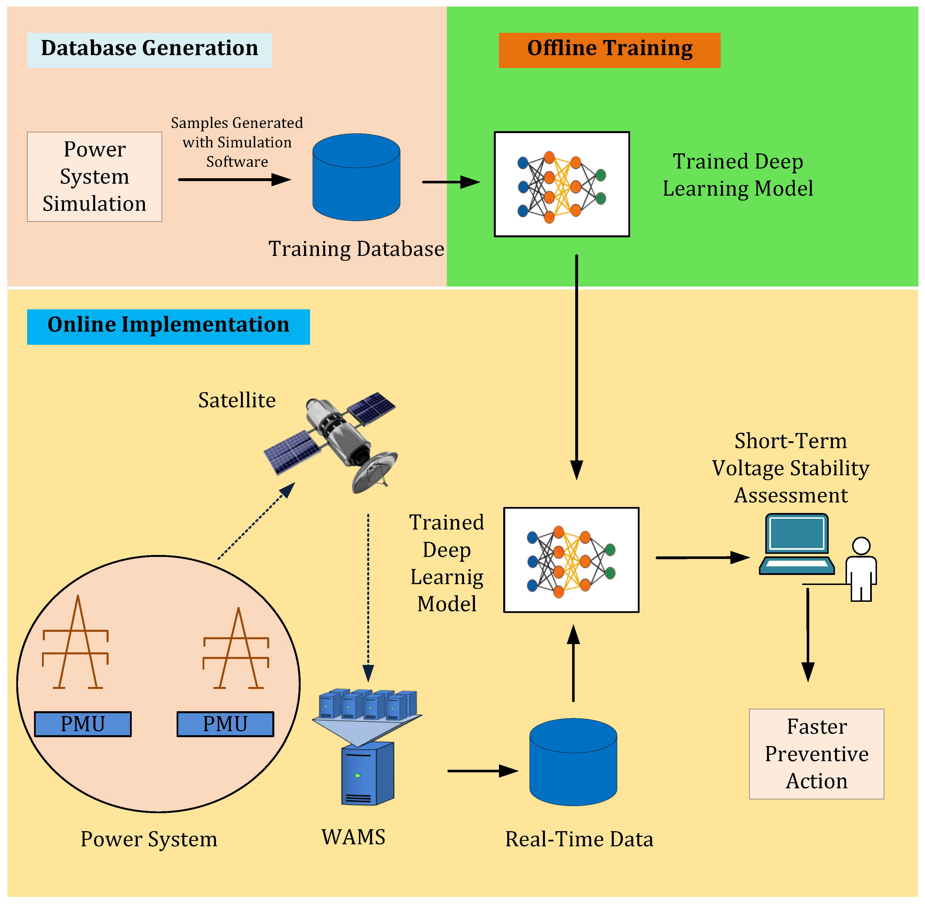
• Proposal of an approach for real-time STVS assessment, including both voltage instability and FIDVR pheomenon based on a deep learning algorithm combining a temporal convolutional neural network and a long short-term memory neural network (TempCNN-LSTM). The proposed TempCNN-LSTM model can extract spatiotemporal STVS features from the data samples available through PMUs.
• The performance of the proposed approach in assessing STVS is compared with other deep learning models and conventional machine learning models under different conditions such as PMUs measurement error, missing PMUs data, and different observation time windows.
• The proposed approach also uses a transfer learning technique for the assessment of STVS that can adapt to the new environment (N-1 contingency case) with a few labeled data samples.

Section 2 describes the theoretical background about the procedure of STVS assessment. The detailed explanation about the proposed TempCNN-LSTM model is given in Section 3. Subsequently, results and discussion for different case studies are presented in Section 4. Finally, the conclusions of this study are summarized in Section 5.

2. Methodology

A general approach of STVS assessment is shown in Figure 1. The training data set is formed by running TDS using power system simulation software. The deep learning model is trained using the samples available through TDS. The trained deep learning model is implemented in the control center for online application. The WAMS transfers the measured data available from PMUs at the remote location to the power system control centers. Then, the trained deep learning model at the control center predicts the STVS state of the power system based on the real-time data available from PMUs. Finally, the operator at the control station can monitor the STVS stability state subjected to large disturbance and make an appropriate control decision.

2.1. Short-Term Voltage Stability Assessment

Figure 2 depicts the structure for implementing the deep learning-based method for STVS assessment. It consists of three stages: database generation, offline training, and online implementation. To represent the possible operating condition of the practical power system, different simulation conditions are run, and the data set is generated. The input are the post-disturbance bus voltage trajectories obtained for the particular operating condition obtained within the OTW. The output are the labeled samples generated with the bus voltage trajectories within the simulation period obtained using TDS. Here, the deep learning model (TempCNN-LSTM) is trained to map the input–output relationship between bus voltage trajectories and the corresponding STVS state of the power system subjected to disturbance. The overall process of the proposed method for the real-time STVS is shown in Figure 3. Finally, at the online implementation stage, the trained deep learning model at the control station predicts the STVS (stable, stable-with FIDVR phenomenon, and unstable) state based on the available samples of post-fault bus voltage trajectories from PMUs without the prior knowledge of which fault occurred in the power system. As a result, preventive measures can be implemented quickly while maintaining the system’s overall stability.

In this study, apart from the TempCNN-LSTM model, other deep learning algorithms such as TempCNN and LSTM and machine learning algorithms such as support vector machine (SVM) and decision tree (DT) are used for model formation. In addition, for the N-1 contingency case, a few labeled data samples are generated to update the trained model in case of a network topology change condition using the transfer learning approach as shown in Figure 2. Finally, the re-trained model is then implemented at the control center to predict the STVS status of the power system.

2.2. Short-Term Voltage Stability Assessment along with Fault-Induced Delayed Voltage Recovery

A large number of data samples are generated by running the comprehensive TDS for a broad range of loading situations, fault locations, and different load dynamics to reflect the practical operating conditions of the power system. The post-fault voltage trajectories samples are obtained for different operating scenarios, and the corresponding labeled samples for each STVS category are evaluated. The database structure is shown in the

Table 1. STVS assessment database structure.

No. of Samples	Bus ID	Input Data (p.u.)				Output (STVS Class)
		Vt1	Vt2	…	Vt
	1	0.45	0.47	…	0.65
1	…	…	…	…	…	0 (Unstable)
	$N_b$	0.67	0.71	…	0.87
	1	0.78	0.81	…	0.97
2	…	…	…	…	…	1 (Stable)
	$N_b$	0.82	0.87	…	0.98
…	…	…	…	…	…	…
	1	0.72	0.75	…	0.96
N	…	…	…	…	…	2 (Stable-with FIDVR)
	$N_b$	0.62	0.68	…	0.97

. Here, N denotes the number of samples, $N_b$ represents the number of buses in a power system, V${}_t$${}_1$ represents the post-fault voltage magnitude at fault clearing time $t_c$, and $V_t$ denotes the post-fault voltage magnitude at the end of the simulation period T. In this study, the simulation time of 5 s is taken for the analysis of STVS assessment. In a database, the input are the post-fault voltage trajectories of each bus over the OTW and the output are the STVS state (stable, unstable, and stable-with FIDVR phenomenon). The FIDVR phenomenon occurs when system voltages remain abnormally low for several seconds after a fault is cleared. The primary cause of these incidents is due to the installation of induction motor loads, which causes a high reactive power demand in the post-fault phase [31]. The FIDVR phenomena is assessed in this study by calculating the transient voltage severity index (TVSI) as [32]:

$$\mathrm{TVSI}=\frac{{\sum }_{k=1}^{N_b}{\sum }_{t=t_{cr}}^{T_o}{\mathrm{TVDI}}_{k,t}}{N_b\times (T_o-t_{cr})}$$

(1)

where $N_b$ is the number of buses in the test system, $T_o$ is the voltage recovery time frame, and $t_{cr}$ is the fault clearing time. The transient voltage deviation index (TVDI) is calculated as follows [32]:

$${\mathrm{TVDI}}_{k,t}=\left\{\begin{array}{cc}\frac{|V_{k,t}-V_{k,0}|}{V_{k,0}},\hfill & \frac{|V_{k,t}-V_{k,0}|}{V_{k,0}}\ge \alpha \forall t\in [t_{cr},T_o]\hfill \\ 0,\hfill & \mathrm{otherwise}\hfill \end{array}\right.$$

(2)

where $V_{k,t}$ at time t and $V_{k,0}$ are the post-fault and the pre-fault voltage magnitude of bus k, respectively. The threshold of permissible voltage deviation magnitude is $\alpha =90\%$ [32], which is frequently employed in industrial criteria. Here, TVSI is used to evaluate the overall system’s voltage stability; a lower value indicates that the system is less susceptible to the FIDVR phenomena. Figure 4 shows a thorough illustration of the STVS phenomena and the labeling process for each sample. If all of the bus voltage trajectories are maintained at or above the pre-fault voltage for a settling time more than 3 s during the full simulation time, the samples are designated as stable [18,33,34]. On the other hand, samples are classified as unstable if the bus voltage trajectories fall below the pre-fault voltage magnitude. For example, if all the bus voltage trajectories of the power system are maintained above 0.9 p.u. at the settling time and over the simulation period, then the power system is in the STVS stable state. If all the bus voltage trajectories fall below 0.9 p.u. or a sustained low voltage without recovery over the simulation interval has occurred, then the power system is in the STVS unstable state. Furthermore, the STVS stable samples are classified into two labels, i.e, stable and stable-with FIDVR phenomenon. The system prone to FIDVR phenomenon is evaluated based on the TVSI. If the TVSI value is greater than 4 [32], it means that the power system is in the state of FIDVR phenomenon subjected to the disturbance. Then, the stable samples are labeled as stable-with FIDVR phenomenon. Similarly, all the samples at different operating scenarios are classified as unstable, stable, and stable-with FIDVR phenomenon, and we labeled each category as 0, 1 and 2, respectively. Overall, all of the samples are represented by their assigned labels, resulting in a multi-class classification problem for STVS evaluation.

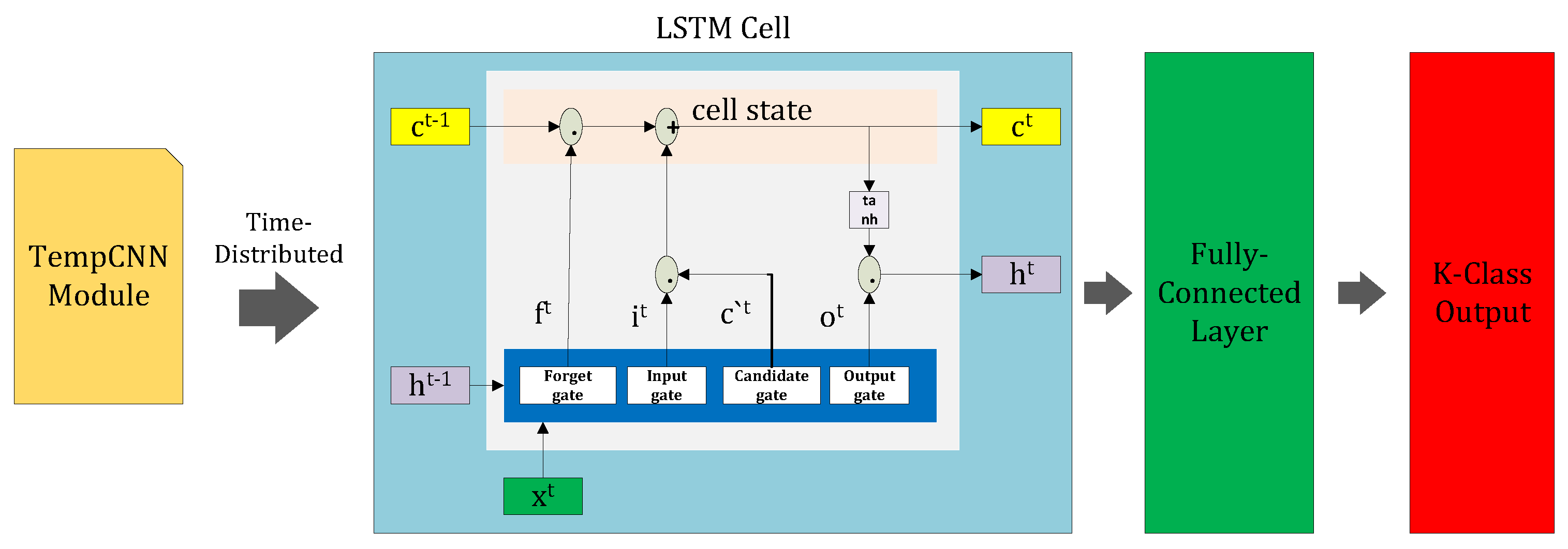
3. Framework of Proposed Temporal Convolutional Neural Network-Long Short-Term Memeory Neural Network

The deep learning model, TempCNN-LSTM, is used for the time series classification (TSC) task. On a data set D, the task of a TSC is to show the relationship between the inputs and the output labels provided by the probability distribution. In a data set $D=((V_1,Y_1),(V_2,Y_2),\dots ,(V_N,Y_N))$ with N number of samples, it is a set of pairs $(V_{N_b},Y_k)$, where $V_{N_b}$ represents the time series voltage trajectories of $N_b$ number of power system buses throughout the OTW length $T_l$ and $Y_k$ represents the system’s STVS state, with $Y_k$ matching to a one-hot label vector. The framework of the proposed TempCNN-LSTM model for the assessment of STVS is shown in Figure 5. To begin, all the PMUs measurement data are collected and pre-processed to reveal the spatiotemporal patterns hidden within the data. The architecture of proposed framework of the TempCNN-LSTM module consists of two deep learning models: the TempCNN and LSTM modules. The TempCNN module extracts and learns spatial information from the data, while the LSTM module handles temporal features. Here, a time-distribute operation is used to combine these models. Then, the TempCNN-LSTM module predicts the existing STVS of the power system after the disturbance. Even with a short period of post-fault voltage trajectories data, the proposed module can anticipate the future condition of a power system. Eventually, a prompt decision can be made to retain the stability state of the system. The combination of deep learning modules TempCNN and LSTM modules are discussed briefly in the preceding section.

3.1. Temporal Convolutional Neural Network

The TempCNN architecture composed of the input layer, two convolution layers, one pooling layer, fully connected layer, and an output layer, as shown in Figure 6, is implemented for TSC task. The spatial and temporal patterns in a raw time series data can be extracted using TempCNN implementing one-dimensional (1-D) filter providing spectro-temporal guidance [15]. When compared to other traditional classification methods, the amount of pre-processing required is significantly less for TempCNN. The following equation represents a general way of applying convolution for the center time stamp t [35]:

$$H_t=g(w\times V_{t-\frac{l}{2}:t+\frac{l}{2}}+b_o),\forall t\in [1,T]$$

(3)

where H denotes the result of convolution on a time series V of length T, w denotes the weights of filter with length l, and g is the non-linear activation function. Here, rectified linear unit (ReLU) function is used for non-linear mapping, and the same convolutional filter value is used for each time stamp to extract the prominent features from the time series data. The pooling layer is used for down sampling the length of input time series data. After the convolution and pooling operation, the original time series is represented by the series of feature maps in a fully connected layer represented by the vectorization layer in Figure 6. Finally, the extracted features from the fully connected layers are input to the LSTM module in a time-distributed manner.

3.2. Long Short-Term Memory Neural Network

An LSTM is adapted for processing the sequential input data. Unlike the recurrent neural network (RNN), LSTM can capture long-term dependencies in time series data with the help of an internal state memory cell [36]. This makes the network learn features of significance. The overall architecture of the LSTM module is shown in Figure 7, which consists of an input gate, forget gate, candidate gate and the output gate. The detail mechanism and operation of the LSTM block can be found in [16,37]. For time series data, an LSTM network may be created by constructing a sequence of many LSTM blocks. The high temporal correlation of the extracted features is handled by the LSTM module. The output vector from the preceding TempCNN module is the input to the LSTM module. In this scenario, the time-distributed technique is employed to reuse the same TempCNN module throughout all input slices. The LSTM layer is used to analyze the input time sequence, learning an implicit correlation between each temporal slice. Furthermore, the output layer has k neurons, corresponding to k class labels. The output layer, which consists of the SoftMax operation, is completely linked to the feature layer. It takes the input time series’ data of voltage trajectories and generates a probability distribution across the data set’s class label. Finally, to train and learn the parameters of the TempCNN-LSTM model, a feed-forward pass followed by backpropagation is applied to minimize the cost function. Here, for a multi-class classification problem, a categorical cross-entropy loss function is used. The Adaptive Moment Estimation (Adam) optimization algorithm [38] is used for training the data set and updating the weights parameters.

3.3. Transfer Learning

In this subsection, the transfer learning approach as shown in Figure 8 is implemented to predict the STVS state in case of a network topology change condition. In transfer learning, the same model trained to solve the STVS state for the source domain (base case) can be utilized to solve the similar task in the target domain (N-1 contingency case) with few labeled data samples. Here, the deep learning model is trained for the base case transfer knowledge to predict the STVS state in case of a network topology change condition, minimizing the categorical cross-entropy loss function. This approach eliminates the need for a large amount of data samples, which are required for training a deep learning model in case of a network topology change condition. Finally, the re-trained deep learning model at the control center can predict the STVS state of the power system.

3.4. Performance Evaluation

Accuracy is used commonly to evaluate the performance of the deep learning and machine learning models for the assessment of STVS [10,14,18]. It is calculated from the confusion matrix in

Table 2. Confusion matrix.

Reference Class	Predicted Class
	Positive	Negative
Positive	True Positive (TP)	False Negative (FN)
Negative	False Positive (FP)	True Negative (TN)

using Equation (4).

$$\mathrm{Accuracy}(\%)=\frac{\mathrm{TP}+\mathrm{TN}}{\mathrm{TP}+\mathrm{FN}+\mathrm{FP}+\mathrm{TN}}\times 100$$

(4)

$$\mathrm{Precision}(\%)=\frac{\mathrm{TP}}{\mathrm{TP}+\mathrm{FP}}\times 100$$

(5)

$$\mathrm{Recall}(\%)=\frac{\mathrm{TP}}{\mathrm{TP}+\mathrm{FN}}\times 100$$

(6)

$$\mathrm{F}1-\mathrm{score}=2\times \frac{\mathrm{Precision}\times \mathrm{Recall}}{\mathrm{Precision}+\mathrm{Recall}}$$

(7)

For uneven distribution of the class labels, the classification accuracy alone might be deceiving. As a result, the confusion matrix as shown in Table 2, which may summarize performance with an unequal class distribution, is also evaluated in this research. For imbalance classification, precision, recall and F1-score measures provide an alternative to classification accuracy. The precision indicates how many positive class predictions are in the positive class. The recall measures how many positive class predictions were made out of all positive class predictions in the data set. Finally, the F1-score provides a single score that balances both the concerns of precision and recall in one number. The greater the F1-score, the better the classifier’s performance. TP, TN, FP, and FN with regard to class instability can be described as follows: the number of samples properly categorized as unstable is TP; the number of samples correctly classified as stable and stable-with FIDVR is TN; the number of samples misclassified as stable and stable-with FIDVR is FN; and the number of samples mistakenly classified as unstable is FP. Furthermore, the performances of these models were compared using the precision Equation (5), recall Equation (6), and F1-score Equation (7).

4. Simulation Result and Discussion

4.1. Test System

This study uses IEEE 9 Bus and New England 39 Bus test systems, as shown in Figure 9 and Figure 10, respectively, for the STVS assessment. The IEEE 9 Bus test system consists of three generators, three loads, six lines, and three transformers. The detailed parameters of this test system can be found in [39]. The New England 39 Bus test system consists of 10 generators, 19 loads, 34 lines, and 12 transformers. The detailed parameters of this test system can be found in [40]. The nations that are leading the way in renewable energy typically have a penetration rate of 20–30% [41]. For this reason, the RESs considered in this study are PVG and WTG, which are assumed to supply 25% of the total electrical demand of the test system. The data and model for RESs are taken from [42,43]. For the IEEE 9 Bus test system, each solar and wind farm of 39 MVA are connected to bus 8. Similarly, for the New England 39 Bus test system, the size of the solar and wind farm at bus 6, 15 and 18 are 297, 263, and 202 MVA, respectively. This study uses the built-in wind farm model and PVG model available in DIgSILENT power factory software [44]. TDS in DIgSILENT power factory software were used to create the data set. To examine the performance of various deep learning and machine learning models, the Keras module with TensorFlow backend in Python is utilized. All the calculations are completed on a PC with an AMD Ryzen 5 2600 Six-Core processor running at 3.40 GHz and 16 GB of RAM.

4.2. Data Generation

To gather voltage magnitude data, the TDS is conducted in IEEE 9 Bus and New England 39 Bus test systems utilizing DIgSILENT power factory software, which considers multiple contingencies under various operating settings. The simulation should capture all the system’s behavior and as many different operating situations as feasible to represent the practical operation condition of the power system. For this, the loading of each bus is varied between 0.8 and 1.2 of its power rating. Similarly, to simulate the uncertainty of RESs, the power generation from the solar and wind farm is varied based on their probability distributions as given in [42,43]. The complex load model in DIgSILENT power factory software, which represents the combination of various load component (static and dynamic loads) is considered for simulation. Here, the complex load model is adapted to represent the dynamics of induction motor loads, which is the primary driving factor for the short-term voltage instability in a power system. The three phase short-circuit faults are assumed to occur at each transmission line. The faults last for 0.1 s and are cleared without the loss of power system elements in this study. The configuration of the data set generation that can resemble the overall operation condition of the power system is outlined in

Table 3. Configuration of data set generation on test systems.

Load level	$\pm 20\%$ of initial loading
Fault lines	All the transmission lines
Load model	Complex load model in DIgSILENT
Load dynamics	0–80% of induction motor load
Fault locations	0–80% of all fault lines
Fault type	Three-phase bolted fault
Fault duration	0.1 s
Simulation time	5 s
Length of OTW	0.25 s of post fault voltage trajectories
Sampling per time step	0.01 s

. For each operating scenario, the simulation is run for 5 s to correctly label the STVS state of the power system. For the IEEE 9 Bus system, a total of 19,450 labeled samples are generated under this condition. Similarly, 20,500 labeled samples are generated for the New England 39 Bus system. To monitor the STVS status of the system, all post-fault voltage samples of time 0.25 s are retrieved from voltage trajectories that resemble the OTW. In this study, the OTW length of 0.25 s is assumed to resemble the longest possible time for the protective device (such as the under-voltage load shedding device) to respond to the post-disturbance condition. The number of sampling points is calculated as the ratio of OTW length to the sampling per time step. Here, the sampling time of 0.01 s is taken, so in total, there are 25 sampling points which resembles the post-fault voltage magnitude at each time step. Therefore, the raw data are an input matrix of size $25\times 9$ for each sample for the IEEE 9 Bus and $25\times 39$ for the New England 39 Bus systems. Each sample has 25 input time series of voltage magnitude and nine variables for the IEEE 9 Bus test system. Similarly, the samples in the New England 39 Bus system have 25 input time series of voltage trajectories and 39 variables representing each bus. Finally, 80% of the data set was randomly selected for training, while 20% was used for validation and testing in this study.

4.3. Analysis of Case Studies

4.3.1. Case I: Base Case

The proposed TempCNN-LSTM is used in this case study to categorize all the phenomena that are present in the STVS assessment. The performance of the proposed model is then compared with other deep learning and conventional machine learning models for both the test systems. According to the data generation by TDS, the training data set for the IEEE 9 Bus test system, there are 19,450 labeled samples: 3514 unstable as class 0, 13,401 stable as class 1, and 2535 stable-with FIDVR as class 2. Similarly, for the training data set for the New England 39 Bus test system, there are 20,500 labeled samples: 4062 unstable as class 0, 12,207 stable as class 1, and 4231 stable-with FIDVR as class 2. All the analysis in this case is conducted with the assessment time of 0.25 s. For the IEEE 9 Bus system, the TempCNN-LSTM model consists of two convolution layers each with 64 units. The TempCNN-LSTM model for New England 39 Bus, on the other hand, is made up of two convolution layers, each with 128 units. For both systems, the filter length of each convolutional layer is set to 3. The learned features are flattened into one long vector after the convolution step. It then passes through an LSTM layer in a time-distributed manner. The LSTM model consists of a single layer with 64 and 128 hidden units for the IEEE 9 Bus system and New England 39 Bus system, respectively, one dense layer and an output layer classify the STVS state of the system. In each layer of both systems’ models, the ReLU activation function is used for non-linear mapping. The SoftMax activation in the output layer gives the probability distribution of each class label, and the class with the highest probability is selected for the particular input samples. The overall model configurations for both test systems are shown in Figure 11. The parameter setting for training the proposed TempCNN-LSTM model is shown in

Table 4. Parameter settings of the proposed TempCNN-LSTM model on test systems.

Parameters	Values
Optimizer	Adam
Exponential decay rate (${\beta }_1$)	0.9
Exponential decay rate (${\beta }_2$)	0.999
Constant ($ϵ$)	10${}^{-7}$
Learning rate	0.001
Batch size	32
Number of epochs	200

. The units in the convolutional layers, filter size, hidden units in the LSTM layer, and dense layer are determined using hyper-parameter optimization using the grid search technique using five-fold cross-validation.

Table 5. Comparison of performance of proposed model with other deep learning and machine learning models.

Test System	Model	Performance Evaluation
		Accuracy	Precision	Recall	F1-Score	Training Time	Testing Time
	Proposed	98.66%	98.74%	98.66%	98.68%	8 min 23 s	406 ms
	TempCNN	97.87%	97.86%	97.87%	97.85%	5 min 59 s	359 ms
IEEE 9 Bus	LSTM	97.86%	97.85%	97.86%	97.81%	19 min 59 s	915 ms
	SVM	92.87%	95.95%	92.87%	93.73%	1 min 9 s	1.2 s
	DT	91.84%	95.42%	91.84%	92.87%	56 s	4.99 ms
	Proposed	96.95%	97.01%	96.95%	96.97%	24 min 42 s	658 ms
	TempCNN	96.44%	96.55%	96.44%	96.47%	9 min 11 s	325 ms
New England 39 Bus	LSTM	96.37%	96.60%	96.36%	96.42%	22 min 54 s	714 ms
	SVM	92.69%	96.82%	92.69%	92.65%	3 min 44 s	1.27 s
	DT	91.36%	92.28%	91.36%	91.48%	3 min 3 s	6 ms

shows the performance of the proposed TempCNN-LSTM model for the prediction of the STVS state of the system in terms of average accuracy, precision, recall, F1-score, training time and testing time. The results show that the proposed model can predict the STVS state with the average accuracy of 98.66% and 96.95% for the IEEE 9 Bus system and New England 39 Bus system, respectively, for a multi-class classification problem. The diagonal of the confusion matrix of the test results, as shown in Figure 12, includes the correctly classified samples of each label for both test systems. In this study, the performance of the proposed model is compared with other popular deep learning and machine learning models such as TempCNN, LSTM, SVM and DT. The result in Table 5 shows that the proposed model outperformed significantly for the multi-class classification task required for the assessment of STVS. Apart from classification accuracy, the proposed model outperformed other models with precision of 98.74%, recall of 98.66%, and F1-score of 98.68% for the IEEE 9 Bus test system with an uneven class distribution of test samples of each category. Similarly, for the New England 39 Bus test system, the proposed model gives a better result with precision of 97.01%, recall of 96.95%, and F1-score 96.97% compared to other classifiers. The results show that the performances of TempCNN and LSTM classifiers are comparable with the proposed model having a marginal difference of accuracy of less than 1%, while the SVM and DT classifiers performed poorly with accuracy less than 93%. The results show that the DT classifier requires less computational time for both the training and testing data set compared to other classifiers for both the test systems under study. Even though the training time required for the proposed model is high, the data processing time for the test samples is quick enough to meet the criterion for online application.

This approach requires the manual labeling of a large number of data samples, which is time consuming in practice and may give a biased result with unknown topology change conditions.

4.3.2. Case II: PMUs Measurement Error Case

The data obtained using PMUs in the real world may contain noise which is normally assumed to be white and Gaussian in nature and thus may lead to taking incorrect action if not considered [45]. The IEEE standard [46] recommends that the total vector error should be less than 1% for the correct functioning of PMUs. This scenario analyzes the impact of the measurement error from PMUs on the prediction capability of the proposed model. The performance of other deep learning models and machine learning models is also analyzed here in terms of test accuracy, precision, recall, and F1-score subjected to the PMUs measurement error. The random noise following the normal distribution with mean zero and the standard deviation of 1% [47] is added to the original database analyzed under the base case condition. The results illustrated in

Table 6. Performance evaluation with PMUs measurement error on test systems.

Test System	Model	Performance Evaluation
		Accuracy	Precision	Recall	F1-Score
	Proposed	97.93%	97.97%	97.93%	97.94%
	TempCNN	97.29%	97.48%	97.29%	97.35%
IEEE 9 Bus	LSTM	97.19%	97.49%	98.18%	97.26%
	SVM	92.75%	95.93%	92.75%	93.64%
	DT	88.71%	93.89%	88.71%	90.38%
	Proposed	96.66%	96.65%	96.66%	96.65%
	TempCNN	95.78%	95.84%	95.78%	95.76%
New England 39 Bus	LSTM	95.02%	95.14%	95.03%	95.06%
	SVM	92.48%	92.64%	92.48%	92.44%
	DT	87.24%	88.53%	87.24%	87.48%

after the addition of noise in both the training and test data sets show that the performance of the proposed model is resilient to the measurement error for both the test systems under study as compared to Table 5. The result shows that the proposed model can classify the STVS state of the power system with the accuracy of 97.93%, and 96.66% for the IEEE 9 Bus test system and New England 39 Bus test system, respectively. It is also found that the performance of all the classifiers decreases with the addition of PMUs noise, with the DT classifier having inferior performance compared to other classifiers in terms of accuracy, precision, recall, and F1-score.

In a practical power system, the PMUs may encounter more severe noise and may lead to incorrect STVS assessment. However, a similar approach as described in this section can be implemented to evaluate the performance of these models in case of severe PMUs measurement error.

4.3.3. Case III: Missing PMUs Data Case

Most of the deep learning and machine learning models fail in prediction when subjected to missing PMUs data, since they require a complete set of features input [48,49]. In a practical power system, the PMUs data become unavailable due to PMUs failure or due to communication latency [50]. In this case, the robustness of different classification models to missing PMUs data is analyzed for online application. To simulate the missing PMUs data for online STVS assessment, a certain portion of the test data set within an OTW is randomly set to NaN (not a number values). Furthermore, the missing bus voltage measurements from PMUs are imputed using k nearest neighbor (kNN) algorithms [47]. Finally, the test set with newly imputed values are used for prediction of the STVS state of the power system using pre-trained models. The STVS state is predicted using 10%, 20%, 30%, 40%, 50%, 60% and 70% of missing data in the test set. The result in Figure 13 shows that there is less influence in the prediction capability of these models with missing PMUs data. The proposed model is more tolerant of missing PMUs data, even when 50% of the data are missing, with an accuracy of more than 97% for both test systems. With merely imputed values using kNN, the missing data condition appears to have a lower impact on the overall classifier performance. Evidently, TempCNN and the LSTM classifier still provide the better accuracy up to 50% of missing data with a marginal difference, while the SVM and DT classifiers’ prediction accuracy is significantly low compared to the proposed model for both the test systems.

However, our work is confined to the assumption that the full observability of a grid is available, and the missing PMUs data can be simply imputed using kNN for online application. In an actual power system, the network topology may change due to fault, and PMUs data may not be available from some buses. In this context, the ensemble-based learning strategy presented in [50] can be applied to handle the issue of network topology changes.

4.3.4. Case IV: Impact of Assessment Time

In this scenario, the performance of the proposed model is evaluated under different assessment times. The input data set is generated for different OTW lengths (0.15 s, 0.25 s and 0.35 s). Then, the performance of the proposed model is compared with other deep learning-based time series classification models (TempCNN and LSTM) and machine learning models (SVM and DT). The result of both the test systems in Figure 14 demonstrate that as the OTW duration is increased, all the models’ performance accuracy improves, with TempCNN-LSTM having greater accuracy than the TempCNN, LSTM, SVM and DT models. Increased assessment time results in more accurate STVS evaluations but less time for remedial response and vice versa. Therefore, there is always a trade-off between the assessment time and model performance accuracy. However, for an online application, a reliable assessment time would be with acceptable accuracy. Specifically, if the acceptable accuracy is assumed to be more than 98%, then for the IEEE 9 Bus system, the proposed model can deliver the STVS status within the OTW of 0.25 s. However, for the New England 39 Bus system, the proposed model can deliver the STVS status reliably only for the OTW of 0.35 s. Similarly, TempCNN and LSTM can provide STVS assessment only for the IEEE 9 Bus system with an OTW of 0.35 s, while for the New England 39 Bus test system, it requires an OTW greater than 0.35 s.

In particular, if reliable accuracy is desired within a short assessment time, then the trade-off solution for an appropriate setting of OTW can be obtained using optimization techniques. However, similar approaches have been discussed in the literature [10], and it is out of scope of our research.

4.3.5. Case V: Transfer Learning for N-1 Contingency Case

In this case, the performance of the proposed TempCNN-LSTM model to the unseen network topology change condition is analyzed for online application using the transfer learning approach. The unseen network condition can be the variation in load pattern, generation, and system topology changes due to contingencies that are not included in the data set during the training process. Here, we have used the N-1 contingency case to represent the network topology change condition subjected to disturbance. For the IEEE 9 Bus system, the critical N-1 contingency is the outage of line 3 connected between bus 5 and 8, which has a maximum loading violation. In total, 260 labeled samples are generated using the data generation configuration as in Table 3 for this test system. Similarly, for the New England 39 Bus test system, the critical N-1 contingency condition is the outage of generator 9 located at bus 38, which has a maximum impact for the loading violation at the transformer connected between bus 6 and 31. The total of 340 labeled samples are generated using the data generation configuration as in Table 3 for this test system. The prediction result of the proposed model for the topology change condition is presented in

Table 7. Comparison of performance using proposed transfer learning method for N-1 contingency case.

Model	Parameter	IEEE 9 Bus		New England 39 Bus
		With TL	Without TL	With TL	Without TL
Proposed	Accuracy	98.08%	66.35%	97.06%	58.82%
	Precision	98.17%	76.92%	97.16%	69.13%
	Recall	98.08%	61.54%	97.06%	58.82%
	F1-Score	97.78%	53.15%	96.59%	45.38%
	Re-Training Time	9.3 s	-	27.2 s	-
	Testing Time	45.7 ms	59 ms	55 ms	57 ms
TempCNN	Accuracy	96.15%	76.92%	95.59%	63.73%
	Precision	98.07%	87.23%	95.13%	72.66%
	Recall	96.15%	76.92%	95.59%	63.72%
	F1-Score	96.75%	74.69%	95.28%	56.16%
	Re-Training Time	8.39 s	-	9.53 s	-
	Testing Time	48.6 ms	71.5 ms	48 ms	142 ms
LSTM	Accuracy	96.15%	61.54%	94.12%	80.88%
	Precision	96.15%	78.71%	94.34%	82.92%
	Recall	96.15%	61.54%	94.12%	80.88%
	F1-Score	96.15%	55.41%	93.65%	79.88%
	Re-Training Time	18.1 s	-	26.5 s	-
	Testing Time	52 ms	188 ms	54 ms	451 ms
SVM	Accuracy	94.23%	59.61%	92.64%	82.35%
	Precision	88.84%	79.01%	87.19%	86.20%
	Recall	94.23%	59.61%	92.06%	82.35%
	F1-Score	91.44%	54.61%	89.83%	81.58%
	Re-Training Time	740 ms	-	3.54 s	-
	Testing Time	2 ms	14 ms	7 ms	71 ms
DT	Accuracy	92.31%	46.15%	92.65%	75.00%
	Precision	97.98%	84.62%	92.70%	83.65%
	Recall	92.31%	46.15%	92.65%	75.00%
	F1-Score	95.06%	49.36%	92.57%	74.74%
	Re-Training Time	1.41 s	-	3.29 s	-
	Testing Time	1 ms	1 ms	1 ms	2 ms

. Here, the classification accuracy of the pre-trained model for the unseen N-1 contingency case is significantly low without transfer learning. However, it can be seen from the table that the same model using transfer learning can predict the STVS state for the N-1 contingency case with the accuracy of 98.08% and 97.06% for the IEEE 9 Bus and New England 39 Bus test systems, respectively, with few numbers of labeled samples. In addition, for the uneven distribution of the class labels in the test samples, the proposed model gives better results with precision of 98.17%, recall of 98.08%, and F1-score of 97.78% for the IEEE 9 bus test system and with precision of 97.16%, recall of 97.06%, and F1-score of 96.59% for the New England 39 bus test system compared to other classifiers. Similarly, the performance of TempCNN seems significantly better followed by LSTM, while SVM and DT have poor performance for both the test systems using the transfer learning approach with few labeled data samples for the N-1 contingency condition. The computational time required for both the training and testing reduces significantly compared to Table 5 using the single deep learning-based transfer learning method; thus, it is suitable for online application.

This case study has only considered a single N-1 contingency to show the application of transfer learning for the unseen topology change condition with few labeled data samples. However, if needed, the approach presented in this section can be simply expanded by creating labeled data samples that account for additional contingencies such as the N-1-1 contingency case.

5. Conclusions

This work proposes a method based on deep learning-based time series classification algorithm TempCNN-LSTM for the online assessment of STVS of the power system with RESs. The proposed method can classify the STVS state: stable or unstable or stable-with FIDVR phenomenon using the post-fault voltage trajectories within a short OTW. The findings of the study are summarized as follows:

• The performance of the proposed model evaluated in terms of classification accuracy shows 98.66% accuracy for the IEEE 9 Bus test system and more than 96.95% accuracy for the New England 39 Bus Test System with efficient computational time for the online assessment of STVS.
• The proposed model shows the superior performance compared to other deep learning models (TempCNN and LSTM) and conventional machine learning models (SVM and DT). The performance of the proposed model in terms of classification accuracy, precison, recall and F1-score is significantly high compared to other classification models.
• The proposed model is more tolerant to the PMUs measurement error/losses and thus is suitable for online assessment of STVS.
• The accuracy of the proposed model under the variation of different assessment time shows the superior performance compared to the existing state-of-art deep learning-based time series classification models (TempCNN and LSTM) and machine learning models (SVM and DT). Furthermore, for all these models, the accuracy increases with the increase in the OTW length.
• Using the deep learning-based transfer learning approach, the proposed model can predict the STVS state of the system under topology change condition (N-1 contingency) with more than 97% accuracy for both the test systems with few labeled samples. It eliminates the need to train different learning models. Furthermore, it reduces the computational time required for re-training the model for online application.

Our future research will investigate the control measure to mitigate the STVS problem in the power system using a data-based approach suitable for online application.

References

1. Kundur, P.; Paserba, J.; Ajjarapu, V.; Andersson, G.; Bose, A.; Canizares, C.; Hatziargyriou, N.; Hill, D.; Stankovic, A.; Taylor, C.; et al. Definition and classification of power system stability IEEE/CIGRE joint task force on stability terms and definitions. IEEE Trans. Power Syst. 2004, 19, 1387–1401. [Google Scholar]
2. Van Cutsem, T.; Vournas, C. Voltage Stability of Electric Power Systems; Springer Science & Business Media: Berlin/Heidelberg, Germany, 1998; Volume 441. [Google Scholar]
3. Potamianakis, E.; Vournas, C. Short-term voltage instability: Effects on synchronous and induction machines. IEEE Trans. Power Syst. 2006, 21, 791–798. [Google Scholar] [CrossRef]
4. Adetokun, B.B.; Muriithi, C.M.; Ojo, J.O. Voltage stability assessment and enhancement of power grid with increasing wind energy penetration. Int. J. Electr. Power Energy Syst. 2020, 120, 105988. [Google Scholar] [CrossRef]
5. Xu, X.; Yan, Z.; Shahidehpour, M.; Wang, H.; Chen, S. Power system voltage stability evaluation considering renewable energy with correlated variabilities. IEEE Trans. Power Syst. 2017, 33, 3236–3245. [Google Scholar] [CrossRef]
6. Liu, K.y.; Sheng, W.; Hu, L.; Liu, Y.; Meng, X.; Jia, D. Simplified probabilistic voltage stability evaluation considering variable renewable distributed generation in distribution systems. IET Gener. Transm. Distrib. 2015, 9, 1464–1473. [Google Scholar] [CrossRef]
7. Prusty, B.R.; Jena, D. A critical review on probabilistic load flow studies in uncertainty constrained power systems with photovoltaic generation and a new approach. Renew. Sustain. Energy Rev. 2017, 69, 1286–1302. [Google Scholar] [CrossRef]
8. Operator, A.E.M. Black System South Australia 28 September 2016. 2017. Available online: https://www.aemo.com.au (accessed on 16 October 2021).
9. Kundur, P.S.; Balu, N.J.; Lauby, M.G. Power System Dynamics and Stability; CRC Press: Boca Raton, FL, USA, 2017; Volume 3. [Google Scholar]
10. Zhang, Y.; Xu, Y.; Dong, Z.Y.; Zhang, R. A hierarchical self-adaptive data-analytics method for real-time power system short-term voltage stability assessment. IEEE Trans. Ind. Inform. 2018, 15, 74–84. [Google Scholar] [CrossRef]
11. Safavizadeh, A.; Kordi, M.; Eghtedarnia, F.; Torkzadeh, R.; Marzooghi, H. Framework for real-time short-term stability assessment of power systems using PMU measurements. IET Gener. Transm. Distrib. 2019, 13, 3433–3442. [Google Scholar] [CrossRef]
12. Gungor, V.C.; Sahin, D.; Kocak, T.; Ergut, S.; Buccella, C.; Cecati, C.; Hancke, G.P. Smart grid technologies: Communication technologies and standards. IEEE Trans. Ind. Inform. 2011, 7, 529–539. [Google Scholar] [CrossRef] [Green Version]
13. Dasgupta, S.; Paramasivam, M.; Vaidya, U.; Ajjarapu, V. Real-time monitoring of short-term voltage stability using PMU data. IEEE Trans. Power Syst. 2013, 28, 3702–3711. [Google Scholar] [CrossRef]
14. Zhu, L.; Lu, C.; Dong, Z.Y.; Hong, C. Imbalance learning machine-based power system short-term voltage stability assessment. IEEE Trans. Ind. Inform. 2017, 13, 2533–2543. [Google Scholar] [CrossRef]
15. Pelletier, C.; Webb, G.I.; Petitjean, F. Temporal convolutional neural network for the classification of satellite image time series. Remote Sens. 2019, 11, 523. [Google Scholar] [CrossRef] [Green Version]
16. Hagmar, H.; Tong, L.; Eriksson, R.; Tuan, L.A. Voltage instability prediction using a deep recurrent neural network. IEEE Trans. Power Syst. 2020, 36, 17–27. [Google Scholar] [CrossRef]
17. Yang, W.; Zhu, Y.; Liu, Y. Fast Assessment of Short-Term Voltage Stability of AC/DC Power Grid Based on CNN. In Proceedings of the 2019 IEEE PES Asia-Pacific Power and Energy Engineering Conference (APPEEC), Macao, China, 4 December 2019; pp. 1–4. [Google Scholar]
18. Zhang, M.; Li, J.; Li, Y.; Xu, R. Deep Learning for Short-Term Voltage Stability Assessment of Power Systems. IEEE Access 2021, 9, 29711–29718. [Google Scholar] [CrossRef]
19. Wang, G.; Zhang, Z.; Bian, Z.; Xu, Z. A short-term voltage stability online prediction method based on graph convolutional networks and long short-term memory networks. Int. J. Electr. Power Energy Syst. 2021, 127, 106647. [Google Scholar] [CrossRef]
20. Li, Y.; Zhang, M.; Chen, C. A deep-learning intelligent system incorporating data augmentation for short-term voltage stability assessment of power systems. Appl. Energy 2022, 308, 118347. [Google Scholar] [CrossRef]
21. Luo, Y.; Lu, C.; Zhu, L.; Song, J. Data-driven short-term voltage stability assessment based on spatial-temporal graph convolutional network. Int. J. Electr. Power Energy Syst. 2021, 130, 106753. [Google Scholar] [CrossRef]
22. Su, H.Y.; Liu, T.Y. Enhanced-Online-Random-Forest Model for Static Voltage Stability Assessment Using Wide Area Measurements. IEEE Trans. Power Syst. 2018, 33, 6696–6704. [Google Scholar] [CrossRef]
23. Zhou, D.Q.; Annakkage, U.D.; Rajapakse, A.D. Online Monitoring of Voltage Stability Margin Using an Artificial Neural Network. IEEE Trans. Power Syst. 2010, 25, 1566–1574. [Google Scholar] [CrossRef]
24. Zheng, C.; Malbasa, V.; Kezunovic, M. Regression tree for stability margin prediction using synchrophasor measurements. IEEE Trans. Power Syst. 2012, 28, 1978–1987. [Google Scholar] [CrossRef]
25. Beiraghi, M.; Ranjbar, A. Online voltage security assessment based on wide-area measurements. IEEE Trans. Power Deliv. 2013, 28, 989–997. [Google Scholar] [CrossRef]
26. Zhuang, F.; Qi, Z.; Duan, K.; Xi, D.; Zhu, Y.; Zhu, H.; Xiong, H.; He, Q. A Comprehensive Survey on Transfer Learning. Proc. IEEE 2021, 109, 43–76. [Google Scholar] [CrossRef]
27. Motiian, S.; Piccirilli, M.; Adjeroh, D.A.; Doretto, G. Unified Deep Supervised Domain Adaptation and Generalization. In Proceedings of the 2017 IEEE International Conference on Computer Vision (ICCV), Venice, Italy, 22–29 October 2017; pp. 5716–5726. [Google Scholar] [CrossRef] [Green Version]
28. Wu, T.; Zhang, Y.J.A.; Wen, H. Voltage Stability Monitoring Based on Disagreement-Based Deep Learning in a Time-Varying Environment. IEEE Trans. Power Syst. 2021, 36, 28–38. [Google Scholar] [CrossRef]
29. Ren, C.; Xu, Y. Transfer Learning-Based Power System Online Dynamic Security Assessment: Using One Model to Assess Many Unlearned Faults. IEEE Trans. Power Syst. 2020, 35, 821–824. [Google Scholar] [CrossRef]
30. Adhikari, A.; Naetiladdanon, S.; Sangswang, A. Real-Time Short-Term Voltage Stability Assessment using Temporal Convolutional Neural Network. In Proceedings of the 2021 IEEE PES Innovative Smart Grid Technologies-Asia (ISGT Asia), Brisbane, Australia, 5–8 December 2021; pp. 1–5. [Google Scholar]
31. Bravo, R.J.; Yinger, R.; Arons, P. Fault induced delayed voltage recovery (FIDVR) indicators. In Proceedings of the 2014 IEEE PES T&D Conference and Exposition, Medellin, Colombia, 10–13 September 2014; pp. 1–5. [Google Scholar]
32. Li, Q.; Xu, Y.; Ren, C. A Hierarchical Data-Driven Method for Event-Based Load Shedding Against Fault-Induced Delayed Voltage Recovery in Power Systems. IEEE Trans. Ind. Inform. 2020, 17, 699–709. [Google Scholar] [CrossRef]
33. Zhu, L.; Lu, C.; Sun, Y. Time series shapelet classification based online short-term voltage stability assessment. IEEE Trans. Power Syst. 2015, 31, 1430–1439. [Google Scholar] [CrossRef]
34. Boričić, A.; Torres, J.L.R.; Popov, M. Fundamental study on the influence of dynamic load and distributed energy resources on power system short-term voltage stability. Int. J. Electr. Power Energy Syst. 2021, 131, 107141. [Google Scholar] [CrossRef]
35. Fawaz, H.I.; Forestier, G.; Weber, J.; Idoumghar, L.; Muller, P.A. Deep learning for time series classification: A review. Data Min. Knowl. Discov. 2019, 33, 917–963. [Google Scholar] [CrossRef] [Green Version]
36. Hochreiter, S.; Schmidhuber, J. Long short-term memory. Neural Comput. 1997, 9, 1735–1780. [Google Scholar] [CrossRef]
37. Greff, K.; Srivastava, R.K.; Koutník, J.; Steunebrink, B.R.; Schmidhuber, J. LSTM: A search space odyssey. IEEE Trans. Neural Netw. Learn. Syst. 2016, 28, 2222–2232. [Google Scholar] [CrossRef] [Green Version]
38. Kingma, D.P.; Ba, J. Adam: A method for stochastic optimization. arXiv 2014, arXiv:1412.6980. [Google Scholar]
39. Shekar, M.C.; Aarthi, N. Contingency Analysis of IEEE 9 Bus System. In Proceedings of the 2018 3rd IEEE International Conference on Recent Trends in Electronics, Information & Communication Technology (RTEICT), Bengaluru, India, 18–19 May 2018; pp. 2225–2229. [Google Scholar]
40. Pai, M. Energy Function Analysis for Power System Stability; Springer Science & Business Media: Berlin/Heidelberg, Germany, 2012. [Google Scholar]
41. Secretariat, R. Global Status Report; REN21 Secretariat: Paris, France, 2018. [Google Scholar]
42. Gurung, S.; Naetiladdanon, S.; Sangswang, A. Probabilistic small-signal stability analysis of power system with solar farm integration. Turk. J. Electr. Eng. Comput. Sci. 2019, 27, 1276–1289. [Google Scholar] [CrossRef]
43. Gurung, S.; Naetiladdanon, S.; Sangswang, A. Coordination of power-system stabilizers and battery energy-storage system controllers to improve probabilistic small-signal stability considering integration of renewable-energy resources. Appl. Sci. 2019, 9, 1109. [Google Scholar] [CrossRef] [Green Version]
44. PowerFactory, D. User Manual; DigSILENT Gmbh: Gomaringen, Germany, 2014. [Google Scholar]
45. Ahmad, T.; Senroy, N. Statistical characterization of PMU error for robust WAMS based analytics. IEEE Trans. Power Syst. 2019, 35, 920–928. [Google Scholar] [CrossRef]
46. Martin, K.E.; Benmouyal, G.; Adamiak, M.; Begovic, M.; Burnett, R.; Carr, K.; Cobb, A.; Kusters, J.; Horowitz, S.; Jensen, G.; et al. IEEE standard for synchrophasors for power systems. IEEE Trans. Power Deliv. 1998, 13, 73–77. [Google Scholar] [CrossRef]
47. Zhu, L.; Hill, D.; Lu, C. Intelligent Short-Term Voltage Stability Assessment via Spatial Attention Rectified RNN Learning. IEEE Trans. Ind. Inform. 2020, 17, 7005–7016. [Google Scholar] [CrossRef]
48. Xu, Y.; Zhang, R.; Zhao, J.; Dong, Z.Y.; Wang, D.; Yang, H.; Wong, K.P. Assessing short-term voltage stability of electric power systems by a hierarchical intelligent system. IEEE Trans. Neural Netw. Learn. Syst. 2015, 27, 1686–1696. [Google Scholar] [CrossRef]
49. Shi, Z.; Yao, W.; Zeng, L.; Wen, J.; Fang, J.; Ai, X.; Wen, J. Convolutional neural network-based power system transient stability assessment and instability mode prediction. Appl. Energy 2020, 263, 114586. [Google Scholar] [CrossRef]
50. Zhang, Y.; Xu, Y.; Zhang, R.; Dong, Z.Y. A missing-data tolerant method for data-driven short-term voltage stability assessment of power systems. IEEE Trans. Smart Grid 2018, 10, 5663–5674. [Google Scholar] [CrossRef]
Figure 1. A general approach of real-time STVS assessment.
Applsci 12 06333 g001
Figure 2. Proposed framework for STVS assessment.
Applsci 12 06333 g002
Figure 3. Proposed method for real-time STVS.
Applsci 12 06333 g003
Figure 4. STVS evaluation and labeling process.
Applsci 12 06333 g004
Figure 5. Framework of proposed TempCNN-LSTM model.
Applsci 12 06333 g005
Figure 6. Temporal convolutional neural network architecture.
Applsci 12 06333 g006
Figure 7. LSTM architecture.
Applsci 12 06333 g007
Figure 8. Transfer learning process.
Applsci 12 06333 g008
Figure 9. IEEE 9 Bus System.
Applsci 12 06333 g009
Figure 10. New England 39 Bus System.
Applsci 12 06333 g010
Figure 11. Architecture of the proposed TempCNN-LSTM model employed on test systems.
Applsci 12 06333 g011
Figure 12. Confusion matrix of test results for the proposed model on test systems.
Applsci 12 06333 g012
Figure 13. Performance with missing PMUs data on test systems.
Applsci 12 06333 g013
Figure 14. Performance with different OTW lengths on test systems.
Applsci 12 06333 g014