Error Correction Method of TIADC System Based on Parameter Estimation of Identification Model

Abstract

The performance of analog-to-digital converters (ADCs) has reached a bottleneck due to the limitations of the manufacturing process and testing environment. Time-interleaved ADC (TIADC) technology can increase the sampling rate without changing the resolution. However, channel mismatch severely degrades the dynamic performance of the TIADC system. For the channel mismatch problem of TIADC, most of the current solutions have preconditions, such as eliminating only some kind of error or increasing the complexity of the hardware. A few methods can estimate multiple errors without changing the hardware circuit. To improve the dynamic performance of the TIADC system, on the basis of an in-depth study of the channel mismatch error of TIADC, according to the system identification theory, an identification model is designed to characterize the frequency characteristics of TIADC. Using the system observation data, the transfer function parameters of the system are recursively estimated. By constructing and verifying the identification model of the TIADC system, and then through the frequency domain correction method, a digital compensation filter is established to complete the error correction of the system. The test results of the four-channel TIADC high-speed data acquisition system show that the actual input and output characteristics of the test system are consistent with the nature of the identification model. The four channels of the TIADC system are provided by four sub-channels of two AD9653 chips, and the highest sampling rate of a single channel is 125MSPS. For sinusoidal input signals from 20 MHz to 150 MHz, the sampling system can achieve a signal-to-noise ratio (SNR) above 56.8 dB and spurious free dynamic range (SFDR) above 69.7 dB. The dynamic performance of the sampling system is nearly equivalent to that of its sub-ADC; the feasibility of the model identification method and the effectiveness of error correction are verified in simulation and experiment.

1. Introduction

Data acquisition systems have been widely used in instrument measurement, communication, aerospace and medical fields [1,2,3,4,5,6,7,8]. As the core component of a data acquisition system, an analog-to-digital converter (ADC) is the only way to achieve analog/digital conversion, the performance of the ADC has a direct impact on the performance of the data acquisition system [9]. With the development of electronic information technology and the increase in the complexity of the testing environment, the frequency and bandwidth of the simulated signal to be tested are getting higher and higher, and at the same time, our requirements for the observation of signal details are also increasing. Forasmuch as these practical factors, we put forward higher requirements for the performance of ADC. The ADC’s performance is primarily determined by two factors: sampling speed and sampling accuracy [10]; the higher the sampling speed of ADC, the higher the frequency of the analog signal that can be collected and the more accurate the real-time change of the analog signal that can be observed; and the higher the sampling accuracy of the ADC, the more accurate the digital quantization of the analog signal. To meet the requirements of real-time sampling and processing of analog signals, the sampling rate of ADC should be improved as much as possible under the condition of a certain sampling accuracy.

Most data acquisition systems designed in practical engineering applications use the multi-channels of a single ADC to complete synchronous acquisition. However, the single-channel performance of ADC has reached a bottleneck, which greatly limits the improvement in the performance of the data acquisition system. For ADC to consider both the high sampling rate and high resolution, high circuit design and manufacturing processes are needed, which greatly increases the cost of data acquisition systems. Therefore, based on the consideration of cost, if we want to maximize the acquisition ability of the data acquisition system, the sampling theory of Time-Interleaved ADC (TIADC) proposed by W.C. Black and D.A. 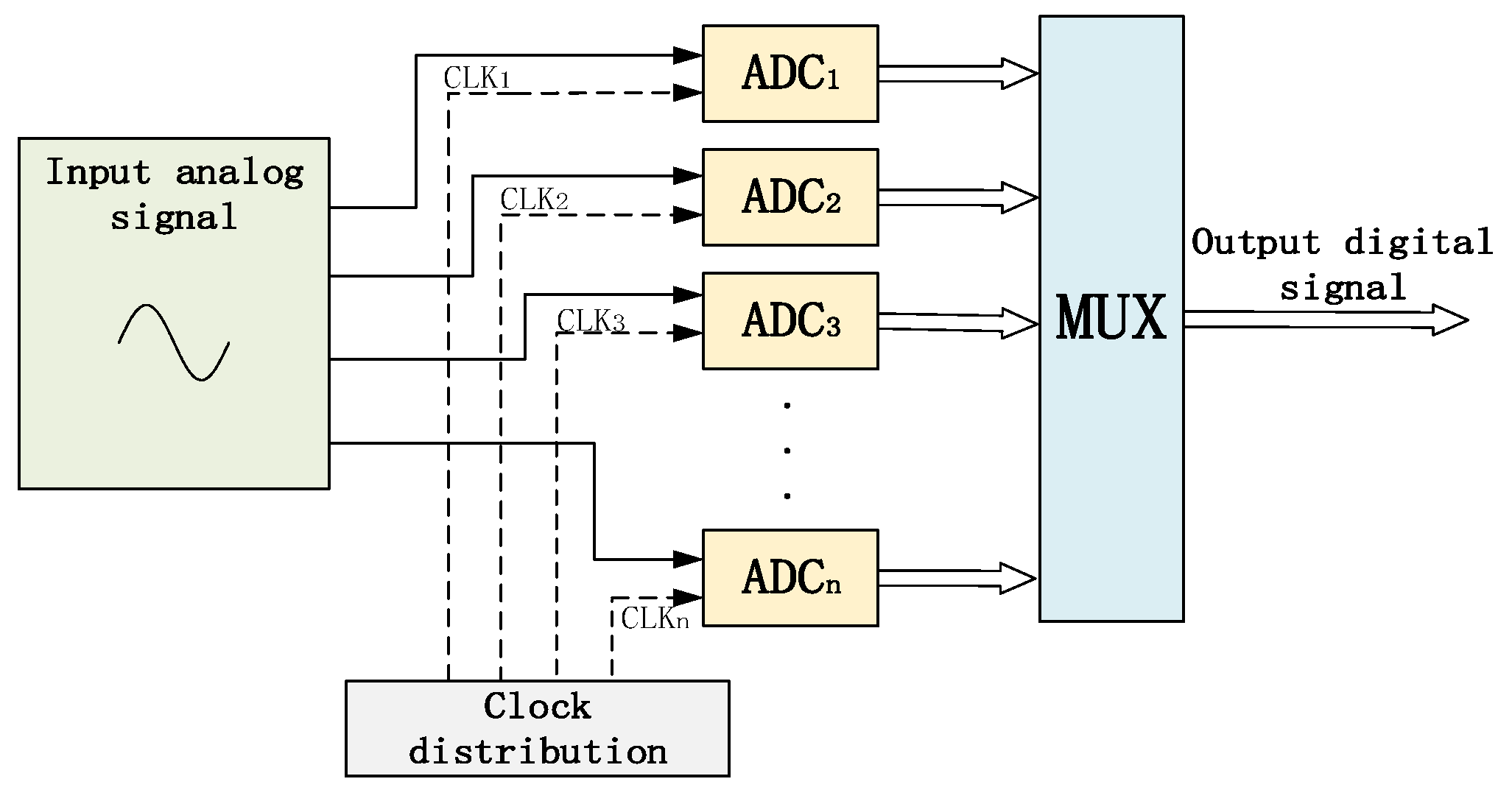Hodges, in 1980, can be used [11]. The basic principle of TIADC is to use several ADCs with low sampling rates to sample a simulated signal under the same clock frequency and different clock phases to improve the sampling rate of the data acquisition system. In the ideal state, the sampling rate of the n-channel TIADC system is n times that of a single sub-ADC. As shown in Figure 1, the working principle diagram of the TIADC system in the ideal state is shown.

Using TIADC sampling technology can greatly improve data acquisition system performance, but it also introduces a new issue—channel mismatch. Bias mismatch, gain mismatch, time mismatch, and bandwidth mismatch are the most common types of channel mismatch [1,12,13,14]. Channel mismatch will seriously reduce the spurious-free dynamic range (SFDR), signal-to-noise ratio (SNR) and distortion rate (SNDR) of the TIADC system. These mismatch errors are derived from the manufacturing process deviation and the physical factors of specific circuits, which are usually difficult to predict and avoid. Therefore, in practical engineering applications, the data acquisition system using TIADC is affected by mismatches, resulting in the deterioration of the dynamic performance of the acquisition system [15].

To solve the problem of a TIADC system caused by channel mismatch, many scholars worldwide have conducted much research on the channel mismatch error of TIADC. In reference [16,17,18], the researchers used a calibration structure with a reference ADC. A premise for using this method is that the accuracy of the reference ADC must be higher than the requirements of TIADC, and its sampling rate must be lower than or even far below TIADC. Although this method can correct the bias and gain mismatch based on statistics, it is powerless for the unstatisticsable sampling time deviation and bandwidth mismatch caused by high-frequency sampling. This method has high complexity and high hardware costs, which are not suitable for practical applications. References [19,20,21] studied the correction structure of reference channel randomization. Since the requirement for noise is lower than that for harmonic or spurious, the reference channel randomization structure is an expedient scheme based on this principle. The randomization structure of the reference channel breaks the regularity of each channel and converts the harmonic or stray energy caused by all non-ideal factors into noise, including bias, gain, bandwidth mismatch and sampling time deviation. However, the reference channel randomization structure only converts harmonics or spurious into noise and does not eliminate these energies. Therefore, failure to really improve performance is the most fundamental flaw in this scheme. In the literature [22,23], the investigators studied the structure of a single preceding Sample-and-Hold Amplifier (pre-SHA), which directly used a single pre-SHA to sample and hold the input signal, and then assigned the retained signal to each sub-ADC in sequence, which no longer needed their own SHA. The single pre-SHA structure not only completely solves the sampling time deviation, but also solves the imbalance, gain and bandwidth mismatch caused by numerous channels; and most importantly, a single pre-SHA determines the entire bandwidth, and this structure almost completely solves the bandwidth mismatch. Although a single pre-SHA structure seems to reduce hardware complexity, it violates the most essential idea of time alternation—parallel processing. For the two-channel TIADC system, the single pre-SHA structure can nearly achieve the requirement of speed doubling, but with the increase in the number of channels, the difficulty of realizing this method will increase to an unimaginable degree. Therefore, in the current research, this structure can only be implemented in a two-channel TIADC system that does not have universal applicability. In References [24,25,26], the split ADC correction structure was used by the researchers; this method is used to correct bias and gain mismatches. The hardware cost is also acceptable, and the method is novel and distinct. However, it still does not solve the correction problem of the sampling time deviation. This structure restricts the correction of sampling time deviation and is appropriate only for low-frequency input conditions with limited bandwidth. For various reasons, such as technology and conditions, many calibration algorithms in the current research are limited by the input signal and do not consider the broadband signal that is more widely used in practice, so they are not universally applicable. While some calibration algorithms improve system performance, they have flaws, such as complex calculations, difficult hardware implementation, resource waste, and so on, and they are also unable to balance performance and cost. In this paper, system identification theory is applied to the TIADC system, which can consider some unknown errors that cannot be quantified and can further improve the correction accuracy of the TIADC system.

The remainder of this paper is introduced briefly as follows: Section 2 proposes a calibration method for TIADC system error based on system identification theory. Section 3 introduces the hardware platform of a 16-bit and four-channel TIADC high-speed data acquisition system used to validate the calibration method’s feasibility. Section 4 provides an overview of the simulation and experimental results. Section 5 is a work summary.

2. Research on the Calibration Method

The identification model is established and analyzed in this section. In order to solve the channel mismatch problem of the TIADC system more effectively and improve the universality of the data acquisition system in various application scenarios, with the analysis of the TIADC system’s structure, this paper designs an identification model to describe the frequency characteristics of the TIADC system based on system identification theory. This process will be elaborated on in Section 2.1. The frequency characteristic parameters of the TIADC system are analyzed in Section 2.2. The recursive parameters are estimated by the method described in Section 2.3, and the identification model is established using the frequency characteristic observation data of the TIADC system. Among them, the larger the input signal frequency range used by the observation frequency characteristics, the more accurate the estimation of the recursive parameters and the wider the scope of application of the system. Finally, in Section 2.4, through the frequency domain correction method, a digital compensation filter is established. 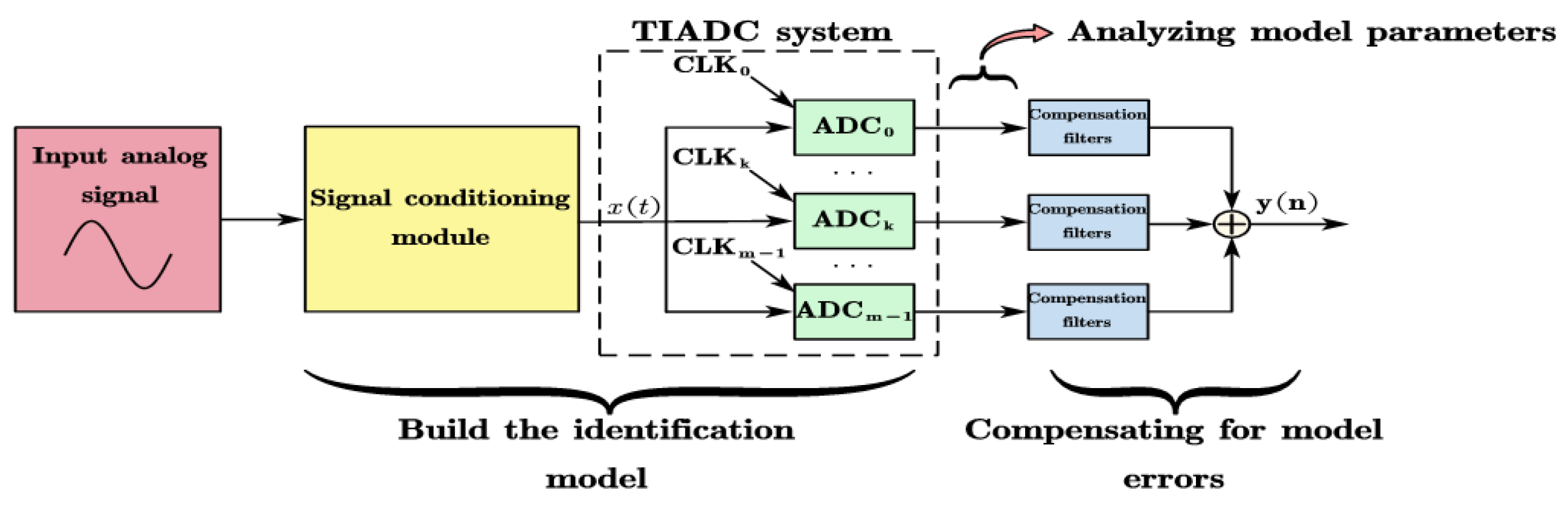In Section 2.5, we summarize the correction methods and expound on the methods to correct the whole TIADC system error. The working mechanism of the TIADC error correction system based on parameter estimation of the identification model is shown in Figure 2. The signal conditioning module in the front-end of analog signal input contains an analog filter, which can reduce the noise of the signal output from the sensor, reduce the order of the identification model, reduce the complexity of digital signal processing and improve the real-time performance of the system.

2.1. Determination and Analysis of the Model Structure

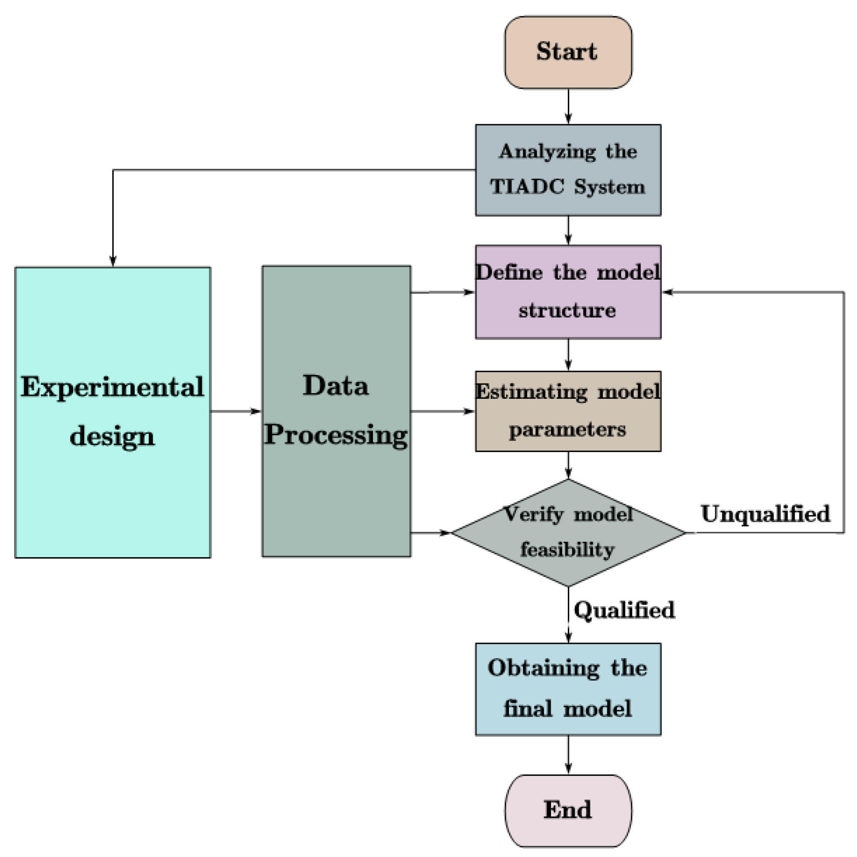
Figure 3 shows the flow chart for the TIADC system to establish an identification model, including experimental design, data processing, system analysis, determination of model structure, parameter estimation, and model verification. First, through the analysis of the TIADC system, a model structure is established, and a reasonable experiment is designed according to the prior knowledge and motion law of the system to ensure that the identification can achieve the desired effect. The data used for identification need to be processed in advance to improve the accuracy of identification and the availability of the identification model. After establishing the structure of the model, the values of some parameters in the model are unknown, so it is necessary to estimate the unknown parameters according to the input and output data. The model obtained by parameter estimation must be verified by the model to test its effectiveness until the performance of the identified model is close to that of the actual system.

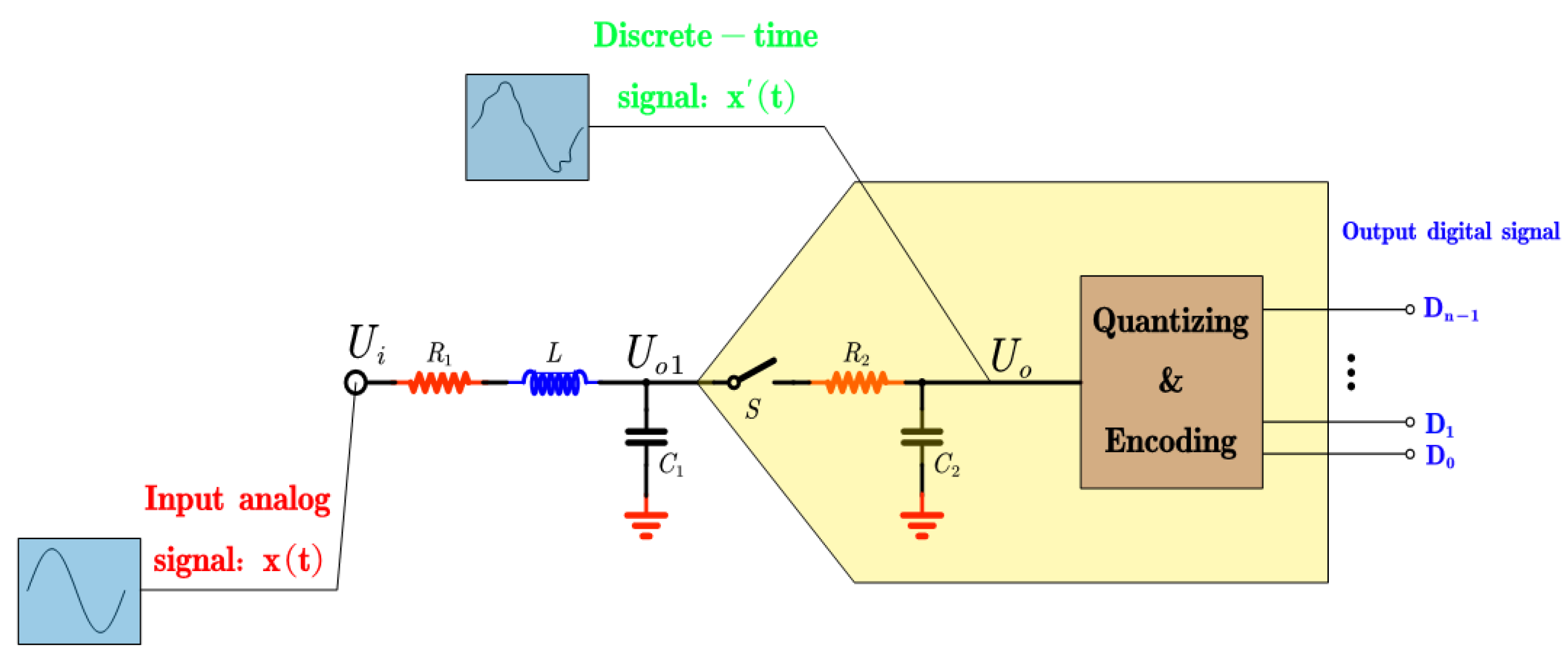
In the TIADC system, if a channel mismatch is not considered, the ADC modules of each channel can be reasonably equivalent to the first-order RC circuit. After experimental verification, the analog filter in the conditioning module can be realized using the second-order RLC circuit. The equivalent model of a single sub-channel in the TIADC system in an ideal state is shown in Figure 4.

First, according to Kirchhoff’s law, the differential equation of the equivalent model circuit of a single sub-channel in a TIADC system under an ideal state is as follows:

$$\{\begin{array}{l}L{C}_1\frac{d^2{U}_{o1}}{d{t}^2}+R_1{C}_1\frac{d{U}_{o1}}{dt}+U_{o1}=U_i\\ R_2{C}_2\frac{d{U}_o}{dt}+U_o=U_{o1}\end{array}$$

(1)

Among them, $U_i$ represents the voltage of the analog input signal, $U_{o1}$ represents the output voltage of the analog input signal after filtering circuit, $U_o$ represents the output voltage of $U_{o1}$ after ADC sampling and keeping the front end.

After Laplace transform of the equivalent model circuit differential equation, it can be transformed into the following form:

$$\{\begin{array}{l}\left(L{C}_1{s}^2+R_1{C}_{1}s+1\right)U_{o1}\left(s\right)=U_i\left(s\right)\\ \left(R_2{C}_{2}s+1\right)U_o\left(s\right)=U_{o1}\left(s\right)\end{array}$$

(2)

From Equation (2), the transfer function equations of the equivalent model of a single sub-channel in the TIADC system under an ideal state can be obtained as follows:

$$\{\begin{array}{l}{G}_1\left(s\right)=\frac{U_{o1}\left(s\right)}{U_i\left(s\right)}=\frac{1}{L{C}_1{s}^2+R_1{C}_{1}s+1}\\ G_2\left(s\right)=\frac{U_o\left(s\right)}{U_{o1}\left(s\right)}=\frac{1}{R_2{C}_{2}s+1}\end{array}$$

(3)

Considering the actual factors, the channel mismatch errors, such as DC bias $\Delta o$, static gain $\Delta g$ and aperture delay $\Delta t$ of each channel are introduced into the ADC equivalent model, as shown in Figure 5.

Let ${\omega }_n=1/\sqrt{L{C}_1}$, $\xi =\frac{R}{2}\sqrt{C_1/L}$, ${\omega }_c=1/R_2{C}_2$, where ${\omega }_n$ denotes the undamped oscillation frequency of the system, $\xi$ denotes the damping ratio of the system, ${\omega }_c$ denotes the cutoff frequency of the system, and $e^{s\Delta t}$ denotes the time delay processes of the system. The values of ${\omega }_n$, $\xi$, ${\omega }_c$ are related to the actual hardware circuit. Then, the transfer function of a single sub-channel in the TIADC system identification model can be expressed as

$$G\left(s\right)=\frac{{\omega }_n^2}{s^2+2\xi {\omega }_{n}s+{\omega }_n^2}\cdot \frac{\left(1+\Delta g\right)e^{s\Delta t}}{s/{\omega }_c+1}+\Delta o$$

(4)

According to the relationship between system frequency characteristics and the transfer function, the frequency response function $G\left(j\omega \right)$ of single sub-channel ADC in the TIADC system identification model can be expressed as follows:

$$G(j\omega )=G(s){|}_{(s=j\omega )}=\frac{{\omega }_n^2}{{\left(j\omega \right)}^2+2\xi {\omega }_{n}j\omega +{\omega }_n^2}\cdot \frac{\left(1+\Delta g\right)e^{\Delta t\cdot j\omega }}{j\omega /{\omega }_c+1}+\Delta o$$

(5)

The time delay process $e^{j\omega △t}$ of the system is expanded in the form of the Taylor series as follows:

$$e^{j\omega \Delta t}=1+j\omega \Delta t+\frac{\Delta t^2}{2}{\left(j\omega \right)}^2+\cdots$$

(6)

In the Equation (6), each power of $j\omega$ denotes that the output of the delay link contains the derivative of the input, because the sample-and-hold structure itself is a first-order structure, and its high-order change rate is very small, so the high-order terms can be omitted, and the approximate form is as follows:

$$e^{j\omega \Delta t}\approx 1+j\omega \Delta t$$

(7)

By combining Equations (5) and (7), the transfer function of the single sub-channel ADC equivalent model in the TIADC system can be expressed as follows:

$$G(j\omega )=\frac{{\omega }_n^2}{{\left(j\omega \right)}^2+2\xi {\omega }_{n}j\omega +{\omega }_n^2}\cdot \frac{\left(1+\Delta g\right)\left(1+j\omega \Delta t\right)}{j\omega /{\omega }_c+1}+\Delta o$$

(8)

2.2. Frequency Characteristic Analysis of the TIADC System Identification Model

In fact, identification is the process of extracting mathematical models from a system’s input and output data. When the order of differential equations is higher, it is very heavy work to decompose denominator polynomials without the aid of computers. Therefore, after establishing a mathematical model of a complex field, the solution to the equation is generally not required. One of the advantages of the Laplace transform is that it can use a graphic method to predict system performance.

To facilitate the estimation of parameters of the TIADC system identification model, the transfer function in Equation (8) can be transformed into the following form:

$$\mathrm{G}(s)=\frac{n_0+n_1(s)+n_2{(s)}^2+\cdots +n_k{(s)}^k}{1+m_1(s)+m_2{(s)}^2+\cdots +m_k{(s)}^k}$$

(9)

In Equation (9), $m_1$, $m_2$,…, $m_k$, $n_1$, $n_2$, $n_3$ and $n_k$ represent the parameters to be identified, and $k$ is the system order-number. For different applications, the order of the identification system may be even or odd. The transformation from Equation (8) to Equation (9) is a completely mathematical process.

The frequency characteristics of the system can be expressed as follows:

$$\mathrm{G}(j\omega )=\frac{n_0+n_1(j\omega )+n_2{(j\omega )}^2+\cdots +n_k{(j\omega )}^k}{1+m_1(j\omega )+m_2{(j\omega )}^2+\cdots +m_k{(j\omega )}^k}$$

(10)

If $k$ is odd, define the parameter vectors and information vectors in Equation (10) as follows:

$${\alpha }_1={\left[m_1,m_3,m_5,\cdots ,m_k\right]}^T\in R^{(k+1)/2}$$

(11)

$${\alpha }_2={\left[m_2,m_4,m_6,\cdots ,m_{k-1}\right]}^T\in R^{(k-1)/2}$$

(12)

$${\beta }_1={\left[n_1,n_3,n_5,\cdots ,n_k\right]}^T\in R^{(k+1)/2}$$

(13)

$${\beta }_2={\left[n_2,n_4,n_6,\cdots ,n_{k-1}\right]}^T\in R^{(k-1)/2}$$

(14)

$$\phi (\omega )={\left[\omega ,-{\omega }^3,{\omega }^5,\cdots ,{(-1)}^{(k-1)/2}{\omega }^k\right]}^T\in R^{(k+1)/2}$$

(15)

$$\psi (\omega )={\left[-{\omega }^2,{\omega }^4,-{\omega }^6,\cdots ,{(-1)}^{(k-1)/2}{\omega }^{k-1}\right]}^T\in R^{(k-1)/2}$$

(16)

If $k$ is even, define the parameter vectors and information vectors in Equation (10) as follows:

$${\alpha }_1={\left[m_1,m_3,m_5,\cdots ,m_{k-1}\right]}^T\in R^{k/2}$$

(17)

$${\alpha }_2={\left[m_2,m_4,m_6,\cdots ,m_k\right]}^T\in R^{k/2}$$

(18)

$${\beta }_1={\left[n_1,n_3,n_5,\cdots ,n_{k-1}\right]}^T\in R^{k/2}$$

(19)

$${\beta }_2={\left[n_2,n_4,n_6,\cdots ,n_k\right]}^T\in R^{k/2}$$

(20)

$$\phi (\omega )={\left[\omega ,-{\omega }^3,{\omega }^5,\cdots ,{(-1)}^{k/2-1}{\omega }^{k-1}\right]}^T\in R^{k/2}$$

(21)

$$\psi (\omega )={\left[-{\omega }^2,{\omega }^4,-{\omega }^6,\cdots ,{(-1)}^{k/2}{\omega }^k\right]}^T\in R^{k/2}$$

(22)

Whether k is odd or even, the transfer function of the system can be expressed by these parameter vectors and information vectors. They can be transformed into the following forms:

$$\begin{array}{cc}\hfill G(j\omega )& =\frac{\left[n_0+{\psi }^T(\omega ){\beta }_2\right]+j{\phi }^T(\omega ){\beta }_1}{\left[1+{\psi }^T(\omega ){\alpha }_2\right]+j{\phi }^T(\omega ){\alpha }_1}\hfill \\ & =\frac{\left[n_0+{\psi }^T(\omega ){\beta }_2+j{\phi }^T(\omega ){\beta }_1\right]\left[1+{\psi }^T(\omega ){\alpha }_2-j{\phi }^T(\omega ){\alpha }_1\right]}{{\left[1+{\psi }^T(\omega ){\alpha }_2\right]}^2+{\left[{\phi }^T(\omega ){\alpha }_1\right]}^2}\hfill \\ & =\mathrm{Re}[G(j\omega )]+jIm[G(j\omega )]\hfill \end{array}$$

(23)

According to Equation (23), the expressions of real part $\mathrm{Re}[G(j\omega )]$ and imaginary part $Im[G(j\omega )]$ of frequency characteristics can be obtained:

$$\mathrm{Re}[G(j\omega )]=\frac{\left[n_0+{\psi }^T(\omega ){\beta }_2\right]\left[1+{\psi }^T(\omega ){\alpha }_2\right]+{\phi }^T(\omega ){\beta }_1{\phi }^T(\omega ){\alpha }_1}{{\left[1+{\psi }^T(\omega ){\alpha }_2\right]}^2+{\left[{\phi }^T(\omega ){\alpha }_1\right]}^2}$$

(24)

$$Im[G(j\omega )]=\frac{\left[1+{\psi }^T(\omega ){\alpha }_2\right]{\phi }^T(\omega ){\beta }_1-\left[n_0+{\psi }^T(\omega ){\beta }_2\right]{\phi }^T(\omega ){\alpha }_1}{{\left[1+{\psi }^T(\omega ){\alpha }_2\right]}^2+{\left[{\phi }^T(\omega ){\alpha }_1\right]}^2}$$

(25)

The real part $\mathrm{Re}[G(j\omega )]$ and imaginary part $Im[G(j\omega )]$ of the frequency characteristics contain all the parameters $n_0$, ${\alpha }_1$, ${\alpha }_2$, ${\beta }_1$ and ${\beta }_2$ of the system to be identified, which are also all the unknown parameters contained in the system transfer function.

The frequency characteristic can also be expressed as the plural form of the sum of the real part and the imaginary part, namely:

$$G(j\omega )=M(\omega )+jN(\omega )$$

(26)

where $M(\omega )$ Called the real frequency characteristic, $N(\omega )$ Called virtual frequency characteristic, $j^2$ = −1.

For the identification problem, using the observed data to construct the criterion function for estimating the unknown parameters is the key to realizing the parameter estimation, and the principle of establishing the criterion function is to realize the minimum error between the observed output and the model output. It can be seen from the frequency characteristic expression that the expressions of the real part and the imaginary part contain all the parameters to be identified in the system, so we can construct the criterion function through the expressions of the real or imaginary frequency characteristics.

2.3. Least Mean Square Parameter Estimation Algorithm Based on Virtual Frequency Characteristics

Because the real frequency characteristic expression is more complex than the virtual frequency characteristic expression, the derived algorithm is more complex in form, so this paper uses the least mean square parameter estimation algorithm based on virtual frequency characteristics.

In the frequency response identification experiment, a sine signal $u\left(t\right)=U\sin \left(\omega t\right)$ with frequency $\omega$ and amplitude $U$ is applied to the input end of the system to be identified, and theoretically $\omega \in \left[0,\infty \right]$. The frequency characteristic observation data $\left\{M\left({\omega }_k\right),N\left({\omega }_k\right)\right\}$ corresponding to each discrete frequency point ${\omega }_k$ (k = 0, 1, 2, …) are collected.

According to Equation (25), the criterion function $J^{*}\left(\vartheta \right)$ based on virtual frequency characteristics is constructed by using the observation data of virtual frequency characteristics $\left\{N\left({\omega }_k\right),k=0,1,2,\cdots \right\}$, which is defined as the square of the difference between the observation data of virtual frequency characteristics $N\left({\omega }_k\right)$ and the model output $Im[G(j\omega )]$.

$$J^{*}(\vartheta )=\frac{1}{2}{\left\{N\left({\omega }_k\right)-Im[\mathrm{G}(j\omega )]\right\}}^2$$

(27)

Transform the expression of virtual frequency characteristics in Equation (25) into the following form:

$$\begin{array}{l}\left\{{\left[1+{\psi }^T(\omega ){\alpha }_2\right]}^2+{\left[{\phi }^T(\omega ){\alpha }_1\right]}^2\right\}Im[G(j\omega )]=\\ \left[1+{\psi }^T(\omega ){\alpha }_2\right]{\phi }^T(\omega ){\beta }_1-\left[n_0+{\psi }^T(\omega ){\beta }_2\right]{\phi }^T(\omega ){\alpha }_1\end{array}$$

(28)

Since the virtual frequency characteristic observation data $N\left({\omega }_k\right)$ contains measurement noise, there is an error between the virtual frequency characteristic observation data $N\left({\omega }_k\right)$ and the model output $Im[G(j\omega )]$. Therefore, according to Equation (28), the equation error expression is defined as:

$$\begin{array}{cc}\hfill v_i\left({\omega }_k\right)& =\left\{{\left[1+{\psi }^T\left({\omega }_k\right){\alpha }_2\right]}^2+{\left[{\phi }^T\left({\omega }_k\right){\alpha }_1\right]}^2\right\}N\left({\omega }_k\right)-\hfill \\ & \left[1+{\psi }^T\left({\omega }_k\right){\alpha }_2\right]{\phi }^T\left({\omega }_k\right){\beta }_1+\left[b_0+{\psi }^T\left({\omega }_k\right){\beta }_2\right]{\phi }^T\left({\omega }_k\right){\alpha }_1\end{array}$$

(29)

The expression of the dynamic data criterion function based on Equation (29) is as follows:

$$J(\vartheta )=\frac{1}{2}{v}_i^2\left({\omega }_k\right)$$

(30)

The estimation of the system parameter $\vartheta =\left[n_0,{\alpha }_1^T,{\alpha }_2^T,{\beta }_1^T,{\beta }_2^T\right]$ when the kth frequency ${\omega }_k$ is input is expressed as:

$$\widehat{\vartheta }\left({\omega }_k\right)={\left[{\widehat{n}}_0\left({\omega }_k\right),{\widehat{\alpha }}_1^T\left({\omega }_k\right),{\widehat{\alpha }}_2^T\left({\omega }_k\right),{\widehat{\beta }}_1^T\left({\omega }_k\right),{\widehat{\beta }}_2^T\left({\omega }_k\right)\right]}^T$$

(31)

Based on the principle of a negative gradient search, the minimum mean square algorithm of parameters $n_0$, ${\alpha }_1$, ${\alpha }_2$, ${\beta }_1$ and ${\beta }_2$ in Equation (9) can be obtained by minimizing the criterion function $J(\vartheta )$:

$${\widehat{n}}_0\left({\omega }_k\right)={\widehat{n}}_0\left({\omega }_{k-1}\right)-\mu \left({\omega }_k\right){\phi }^T\left({\omega }_k\right){\widehat{\alpha }}_1\left({\omega }_{k-1}\right){\widehat{v}}_i\left({\omega }_k\right)$$

(32)

$$\begin{array}{c}{\widehat{\alpha }}_1\left({\omega }_k\right)={\widehat{\alpha }}_1\left({\omega }_{k-1}\right)-\mu \left({\omega }_k\right)[2N\left({\omega }_k\right){\phi }^T\left({\omega }_k\right){\widehat{\alpha }}_1\left({\omega }_{k-1}\right)+\\ {\widehat{n}}_0\left({\omega }_{k-1}\right)+{\psi }^T\left({\omega }_k\right){\widehat{\beta }}_2\left({\omega }_{k-1}\right)]\phi \left({\omega }_k\right){\widehat{v}}_i\left({\omega }_k\right)\end{array}$$

(33)

$$\begin{array}{c}{\widehat{\alpha }}_2\left({\omega }_k\right)={\widehat{\alpha }}_2\left({\omega }_{k-1}\right)-\mu \left({\omega }_k\right)[2N\left({\omega }_k\right)+2N\left({\omega }_k\right){\psi }^T\left({\omega }_k\right)\cdot \\ {\widehat{\alpha }}_2\left({\omega }_{k-1}\right)-{\phi }^T\left({\omega }_k\right){\widehat{\beta }}_1\left({\omega }_{k-1}\right)]\psi \left({\omega }_k\right){\widehat{v}}_i\left({\omega }_k\right)\end{array}$$

(34)

$${\widehat{\beta }}_1\left({\omega }_k\right)={\widehat{\beta }}_2\left({\omega }_{k-1}\right)+\mu \left({\omega }_k\right)\left[1+{\psi }^T\left({\omega }_k\right){\widehat{\alpha }}_2\left({\omega }_{k-1}\right)\right]\phi \left({\omega }_k\right){\widehat{v}}_i\left({\omega }_k\right)$$

(35)

$${\widehat{\beta }}_2\left({\omega }_k\right)={\widehat{\beta }}_2\left({\omega }_{k-1}\right)-\mu \left({\omega }_k\right){\phi }^T\left({\omega }_k\right){\widehat{\alpha }}_1\left({\omega }_{k-1}\right)\psi \left({\omega }_k\right){\widehat{v}}_i\left({\omega }_k\right)$$

(36)

$$\begin{array}{cc}\hfill {\widehat{v}}_i\left({\omega }_k\right)& =\{{\left[1+{\psi }^T\left({\omega }_k\right){\widehat{\alpha }}_2\left({\omega }_{k-1}\right)\right]}^2+{\left[{\phi }^T\left({\omega }_k\right){\widehat{\alpha }}_1\left({\omega }_{k-1}\right)\right]}^2\}N\left({\omega }_k\right)-\hfill \\ & \left[1+{\psi }^T\left({\omega }_k\right){\widehat{\alpha }}_2\left({\omega }_{k-1}\right)\right]{\phi }^T\left({\omega }_k\right){\widehat{\beta }}_1\left({\omega }_{k-1}\right)+\hfill \\ & \left[{\widehat{n}}_0\left({\omega }_{k-1}\right)+{\psi }^T\left({\omega }_k\right){\widehat{\beta }}_2\left({\omega }_{k-1}\right)\right]{\phi }^T\left({\omega }_k\right){\widehat{\alpha }}_1\left({\omega }_{k-1}\right)\hfill \end{array}$$

(37)

$$\mu \left({\omega }_k\right)=\underset{\mu ⩾0}{argmin}J\left(\widehat{g}\left({\omega }_{k-1}\right)-\mu g_k\right)$$

(38)

$$\begin{array}{cc}\hfill g_k& =grad\left[J\left(\vartheta \left({\omega }_{k-1}\right)\right)\right]\hfill \\ & =[\frac{\partial J\left(\widehat{\vartheta }\left({\omega }_{k-1}\right)\right)}{\partial n_0},\frac{\partial J\left(\widehat{\vartheta }\left({\omega }_{k-1}\right)\right)}{\partial {\alpha }_1^T},\frac{\partial J\left(\widehat{\vartheta }\left({\omega }_{k-1}\right)\right)}{\partial {\alpha }_2^T},\frac{\partial J\left(\widehat{\vartheta }\left({\omega }_{k-1}\right)\right)}{\partial {\beta }_1^T},\frac{\partial J\left(\widehat{\vartheta }\left({\omega }_{k-1}\right)\right)}{\partial {\beta }_2^T}]\hfill \end{array}$$

(39)

$$\widehat{\vartheta }\left({\omega }_k\right)={\left[{\widehat{n}}_0\left({\omega }_k\right),{\widehat{\alpha }}_1^T\left({\omega }_k\right),{\widehat{\alpha }}_2^T\left({\omega }_k\right),{\widehat{\beta }}_1^T\left({\omega }_k\right),{\widehat{\beta }}_2^T\left({\omega }_k\right)\right]}^T$$

(40)

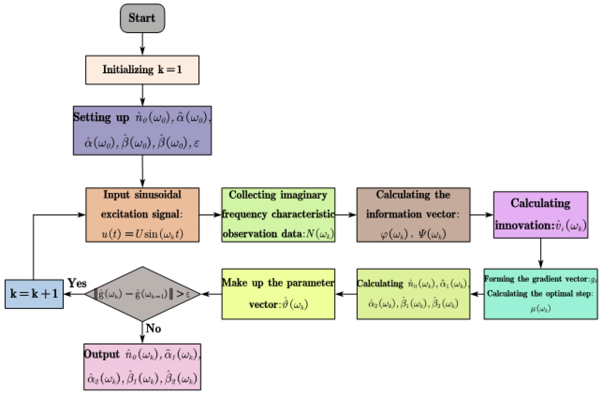
To sum up, the steps of estimating system transfer function parameters based on the least mean square parameter estimation algorithm of virtual frequency characteristics are as follows: the specific process is shown in Figure 6.

• Initialization: make $k$ = 1, set the initial value ${\widehat{n}}_0\left({\omega }_0\right)$ to any real number, ${\widehat{\alpha }}_1\left({\omega }_0\right)$, ${\widehat{\alpha }}_2\left({\omega }_0\right)$, ${\widehat{\beta }}_1\left({\omega }_0\right)$ and ${\widehat{\beta }}_2\left({\omega }_0\right)$ to any real vector, and set the parameter estimation precision $\epsilon$.
• A sinusoidal excitation signal is applied to collect the observed data $N({\omega }_k)$ of virtual frequency characteristics.
• Consider $k$ as odd or even and calculate the information vectors $\phi ({\omega }_k)$ and $\psi ({\omega }_k)$ with Equations (15) and (16) or (21) and (22).
• Calculate the innovation using Equation (37).
• The gradient vector $g_k$ is calculated and formed by Equation (39), and the optimal step size $\mu \left({\omega }_k\right)$ (approximate step size can be taken) is calculated by Equation (38).
• Use Equation (32) to calculate parameter estimation ${\widehat{n}}_0\left({\omega }_k\right)$, Equation (33) to calculate parameter estimation ${\widehat{\alpha }}_1\left({\omega }_k\right)$, Equation (34) to calculate parameter estimation ${\widehat{\alpha }}_2\left({\omega }_k\right)$, Equation (35) to calculate parameter estimation ${\widehat{\beta }}_1\left({\omega }_k\right)$, and Equation (36) to calculate parameter estimation ${\widehat{\beta }}_2\left({\omega }_k\right)$.
• The parameter vector $\widehat{\vartheta }\left({\omega }_k\right)$ is formed by Equation (40).
• If $\Vert \widehat{g}\left({\omega }_k\right)-\widehat{g}\left({\omega }_{k-1}\right)\Vert >\epsilon$, $k$ increases by 1, and go to step 2; otherwise, output parameter estimation ${\widehat{n}}_0\left({\omega }_k\right)$, ${\widehat{\alpha }}_1\left({\omega }_k\right)$, ${\widehat{\alpha }}_2\left({\omega }_k\right)$, ${\widehat{\beta }}_1\left({\omega }_k\right)$, ${\widehat{\beta }}_2\left({\omega }_k\right)$ and terminate the cycle calculation process.

2.4. Frequency Domain Correction Method

After the parameter estimation and verification of the identification model of the TIADC system is completed, we obtain an identification model with dynamic performance close to the actual hardware system. To improve the dynamic performance of the TIADC system, eliminating the dynamic error of the system is the first issue to be considered. When the transfer function of the measurement system is $G\left(s\right)$ and the Laplace transform of the measured signal is $X\left(s\right)$, the dynamic error of the measurement results is as follows:

$$\Delta Y\left(s\right)=\left[G\left(s\right)-G\left(0\right)\right]X\left(s\right)$$

(41)

Equation (41) shows that the dynamic error of the system is related to the dynamic characteristics of the measurement system and the spectrum structure of the measured signal. The frequency domain correction method calculates the spectrum $X\left(j\omega \right)$ of the measured signal from the frequency characteristic $G\left(j\omega \right)$ of the test system and the spectrum $Y\left(j\omega \right)$ of the measured signal, and then uses the inverse Fourier transform to obtain the estimated value of the measured signal, which can be expressed as:

$$\widehat{x}\left(t\right)=IFFT\left[Y\left(j\omega \right)/G\left(j\omega \right)\right]$$

(42)

Next, the discrete transfer function of the TIADC system is used to directly recover the measured signal from the measured results using the deconvolution method, and good results can be obtained. The calculation of this algorithm is relatively small, and most of the calculations can be carried out in advance before the experiment. Therefore, it can be used in online test corrections or test data processing systems.

Suppose $x\left(t\right)$ is the input analog signal, and $y\left(t\right)$ is the measurement result of the TIADC system. According to the bilinear transformation method, the transfer function of the TIADC system can be discretized and transformed into the following form:

$$G\left(z^{-1}\right)=\frac{b_0+b_1{z}^{-1}+b_2{z}^{-2}+\cdots +b_m{z}^{-m}}{1+a_1{z}^{-1}+a_2{z}^{-2}+\cdots +a_n{z}^{-n}}$$

(43)

When Equation (43) is described by the difference equation, it can be expressed as:

$$x\left(k\right)=\frac{1}{b_0}\left[y\left(k\right)+{\displaystyle \sum _{i=1}^n{a}_{i}y\left(k-i\right)-{\displaystyle \sum _{i=1}^m{b}_{i}y\left(k-i\right)}}\right]$$

(44)

In Equation (44), $x\left(k\right)$, $y\left(k\right)$ are sampled values of $x\left(t\right)$, $y\left(t\right)$, respectively.

Equation (44) shows that the measured signal can be recovered from the measured signal with the discrete transfer function of the TIADC system. Among them, the sampling interval $\Delta T$ of $y\left(k\right)$ should be consistent with the switching period $\Delta T_0$ (i.e., the sampling interval of the analog/digital converter) of the discrete system $G\left(z^{-1}\right)$. Therefore, before the experiment is conducted, every sampling interval $\Delta T$ is selected, and the discrete transfer function must be calculated by the continuous transfer function $G\left(s\right)$.

2.5. Summary of Calibration Methods

The error estimation and correction of any single channel of the TIADC system can be realized in Section 2.1, Section 2.2, Section 2.3 and Section 2.4. Through the strict distribution and management of the phase and clock of each channel of the TIADC system, after the error correction of each channel is completed, the output of each channel is merged to realize the output correction of the TIADC system.

3. Construction of the Experimental Platform

To verify the feasibility of the model identification method and the effectiveness of compensation, this section introduces a 16-bit, four-channel TIADC high-speed data acquisition system hardware platform. This hardware platform is mainly composed of an FPGA (XC7K410T) processing motherboard, a collection board containing two AD9653 chips, a clock board, a power divider and a computer. The clock board is configured by the host computer to generate the sampling clock and phase required by each sub-channel of the TIADC acquisition system, and a sinusoidal signal is generated as the analog input signal of the acquisition system. The analog signals are connected to the power divider and divided into four signals, which are sent to four ADC sub-channels. The data collected by the ADC acquisition board are sent to the DDR3 cache after FPGA preprocessing, and the cached data are transmitted to the computer through the USB3.0 data post-processing interface. Figure 7 shows the overall structure of the TIADC data acquisition system.

4. Verification of the Identification Model and Compensation

After the estimation of all the unknown parameters contained in the transfer function of the TIADC system is completed, the results of system identification are verified in this section. Through the electronic test of the four-channel TIADC data acquisition system, the accuracy of the parameter estimation algorithm was verified.

The test standard for ADC is IEEE 1241–2010 [27]. According to this standard, the sine wave can be used for testing, mainly because the sine wave frequency is single, and spectrum analysis can intuitively observe the characteristics of the system. The digital signal converted by the ADC system can be used to calculate its static performance parameters by histogram statistical analysis. The spectrum can also be directly obtained through FFT analysis, and then its dynamic performance parameters can be calculated.

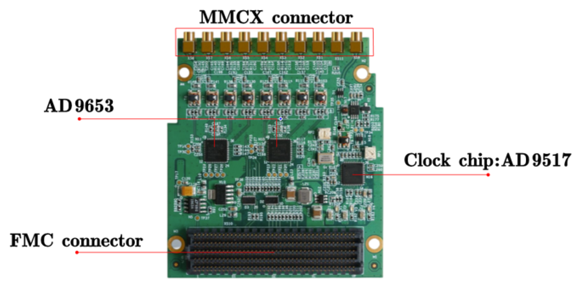
To verify the proposed parameter estimation method, the TIADC data acquisition system mentioned in Section 3 is tested. The four ADC channels used in the TIADC system are realized by two AD9653 chips, and a single frequency sine wave is generated by the clock board. The TIADC test system is shown in Figure 8, and the ADC acquisition card is shown in Figure 9.

By identifying and analyzing the four sub-channel models of the acquisition system, a comparison of the characteristic curves between the model of the acquisition system and the actual input and output can be obtained, as shown in Figure 10. It can be seen from the comparison of amplitude-frequency and phase-frequency curves of four sub-ADC channels that the trend of the results of the identified model is similar to the experimental data, which shows the feasibility and validity of this proposed method.

Due to the existence of gain mismatch and phase mismatch, spurious will appear in the spectrum of 30 MHz, 83.3 MHz and 136.4 MHz. The output spectrum of the 150 MHz sinusoidal signal before and after compensation is shown in Figure 11. For sinusoidal input signals from 20 MHz to 150 MHz, after calibration by the TIADC system, SNR above 59 dB and SFDR above 68 dB can be obtained. SNR increased by more than 12 dB, and SFDR increased by more than 13 dB. The dynamic performance of the TIADC system is close to that of its sub-ADC, indicating the effectiveness of this method.

In

Table 1. Comparison of the correction effects of the methods in [28] and in this article.

Method	SNR/dB	SFDR/dB
Method used in this article	59.1	68.9
Method used in [28]	56.4	70.3

, we compare the method in reference [28] with the method in this paper. After the correction of these two methods, the dynamic performance of the TIADC system used in this paper is very close, which further proves the feasibility of this method in this paper.

5. Conclusions

This paper presents a parameter estimation and calibration method for the TIADC system identification model. According to system identification theory, the TIADC system identification model is established. The least mean square estimation algorithm is used to estimate the parameters related to the system frequency characteristics, and the digital compensation filter is established through the frequency domain correction method to correct the error of the TIADC system. A 16-bit, four-channel TIADC data acquisition system is used to verify the proposed method. Through simulation and experiments, the actual input and output characteristics of the data acquisition system are consistent with the nature of the identification model, and the digital compensation filter established by the frequency domain correction method has high correction accuracy. The data acquisition system can achieve SNR above 59.1 dB and SFDR above 68.9 dB in the input signal from 150 MHz. SNR increases more than 12 dB, SFDR increases more than 13 dB, and the dynamic performance of the system is close to its sub-ADC dynamic performance. The experimental results show the feasibility of the model identification method and the effectiveness of error correction.