
Application of Continuous Non-Gaussian Mortality Models with Markov Switchings to Forecast Mortality Rates


Department of Mathematics and Natural Sciences, Cardinal Stefan Wyszynski University, Woycickiego 1/3, 01-938 Warsaw, Poland
*
Author to whom correspondence should be addressed.
Appl. Sci. 2022, 12(12), 6203; https://doi.org/10.3390/app12126203
Submission received: 11 May 2022
/
Revised: 11 June 2022
/
Accepted: 14 June 2022
/
Published: 18 June 2022
(This article belongs to the Special Issue Applied Biostatistics & Statistical Computing)
Abstract
:Featured Application
The proposed new methods of modelling and forecasting mortality rates are used, among others, to estimate life expectancy depending on the type of death as a fundamental life insurance factor.
Abstract
The ongoing pandemic has resulted in the development of models dealing with the rate of virus spread and the modelling of mortality rates . A new method of modelling the mortality rates with different time intervals of higher and lower dispersion has been proposed. The modelling was based on the Milevski–Promislov class of stochastic mortality models with Markov switches, in which excitations are modelled by second-order polynomials of results from a linear non-Gaussian filter. In contrast to literature models where switches are deterministic, the Markov switches are proposed in this approach, which seems to be a new idea. The obtained results confirm that in the time intervals with a higher dispersion of , the proposed method approximates the empirical data more accurately than the commonly used the Lee–Carter model.
1. Introduction
The existing SARS-CoV-2 pandemic has resulted in the growth of epidemiological models that mainly describe the virus’s evolution and spread, affecting many public life spheres (social, economic, institutional, administrative, etc.). The most frequently used tools for building these models last year include: machine learning, taking into account various types of regression (e.g., multivariate regression, SVM, Cox multivariate regression, LASSO binary logistic regression [1], etc.). Other methods are based, e.g., on autoregressive models (ARiMA [2]), which also include the commonly used the Lee–Carter model (abbreviated as the LC model, [3,4,5,6,7]). Recently, mortality models described by stochastic differential equations have also been developed ([8,9,10]), including COVID-19 models ([11,12,13]).
This group of methods can be divided into two subgroups: the first subgroup consists of mortality models without jumps [14,15,16,17,18], while the second group consists of the ones with jumps [15,19,20,21].
Nowadays, the high dynamics of changes also force adjusting their parameters to the forecasting models’ situations. Therefore, it can be observed that there is still a need to search for models that consider the variability of parameters over time. Some authors have proposed using the methodology of stochastic dynamic hybrid (switched) systems ([22,23]). They considered the dynamic systems to consist of several subsystems described by deterministic or stochastic differential equations. These subsystems have the same structures and different parameters. The submodels can change over time according to a given switching rule, creating a hybrid system.
Recently, this idea was developed by [24,25,26], where the authors proposed measure changes (probability distributions) for LC-models. Another approach was developed by [27,28,29,30,31,32]. The authors proposed extended Milevsky and Promislov models with the non-Gaussian linear scalar filters for modelling of empirical mortality coefficients (). Compared to the Gaussian linear scalar filters model with switchings (GLSFs) and Lee–Carter with switchings (LCs), the model proposed above allows for a more precise estimate of for some fixed age groups of X. The proposed models with switchings seem to represent the natural way the epidemic oscillates. Unfortunately, the switching times were assumed to be deterministic in all mentioned approaches ([33]).
In this paper, we first propose a special case when the empirical data of can be divided into three basic parts. The observed data are “regular” (lower dispersion) in their first and third part. The second part is “nonregular”, chaotically distributed, and with higher dispersion. The mortality models corresponding to the first and third part of the observed data are assumed to be extended Milevsky and Promislow models with the non-Gaussian linear scalar filters. The Markov switched model is proposed for the second part of the empirical data, which is a consequence of the switching between the first and the third part of the observed data. We will use the first and second moments of mortality rates in an iterative procedure to estimate the model parameters and the switching points between three basic parts. To the author’s knowledge, the proposed approach is a new one.
The paper is organised as follows. In Section 2.1, basic notations and definitions of stochastic hybrid systems with Markov switchings are introduced. In Section 2.2 and Section 2.3, two new basic models with Gaussian linear scalar filters and continuous non-Gaussian excitation are presented, respectively. The moment equations are derived, and the stationary solutions for part variables are found. It is shown that only some of the parameters of these models can be unambiguously estimated. In Section 2.4, parameter estimation is performed based on the adapted numerical algorithm of a nonlinear minimisation problem (random search). The hybrid models are obtained by: parameter estimation procedures and the determination of switching points based on the Chow test for both models. The following steps of the technical work in Section 2.1, Section 2.2, Section 2.3 and Section 2.4 were performed:
- S1.
- The family of extended Milevsky and Promislov mortality models with Gaussian linear scalar filters (GLSF) is studied. This family is described by stochastic processes representing a mortality rate for a person aged X at time t. The solutions of the mentioned stochastic differential equations are considered with switches (Section 2.1).
- S2.
- Considering the ln-function of , and applying the Ito formula, a new vector state with unknown parameters is introduced (Section 2.2).
- S3.
- Using moment equations for GLSF with Markov switches, the first- and the second-order moments of equations for a particular case of two subsystem models (stationary and nonstationary solutions) are obtained, and approximate solutions are analysed (Section 2.2.1, Section 2.2.2 and Section 2.2.3).
- S4.
- A similar analysis to step S3 for the non-Gaussian linear scalar filters (nGLSF) model with Markov switches is repeated (Section 2.3).
- S5.
- The estimation procedure of the parameters (introduced in step S2) is applied (Section 2.4).
In Section 3, we have compared empirical mortality rates with theoretical ones obtained from the standard LC model and the models proposed in Section 2.1. Section 4 contains the discussion. Conclusions research are then given in Section 5.
2. Materials and Methods
2.1. Mathematical Preliminaries
Throughout this paper, we use the following notation. Let and <·> be the Euclidean norm and the inner product in , respectively. We mark , . Let be a complete probability space with a filtration satisfying usual conditions. Let be the switching rule, where is the set of states. We denote switching times as and assume that there is a finite number of switches on every finite time interval. Let be the independent Brownian motions. We assume that processes and are both adapted.
By the stochastic hybrid system, we call the vector Itô stochastic differential equations with a switching rule described by
where is the state vector, is an initial condition, and M is a number of Brownian motions. and are defined by sets of and , respectively, i.e., , for . Functions f: and are locally Lipschitz and such that . These conditions together with these enforced on the switching rule ensure that there exists a unique solution of hybrid system (1).
Hence, it follows that Equation (1) can be treated as a family (set) of subsystems defined by
where is the state vector of the l-subsystem.
We assume that processes and are mutually independent and both are adapted. Let , be a right-continuous Markov chain on the probability space taking values in a finite state space with the generator , i.e.,
where , is the transition rate from i to j if , . We assume that the Markov chain is irreducible, i.e., rank , and has a unique stationary distribution , which can be determined by solving
2.2. Model with Gaussian Linear Scalar Filter (GLSF)
We consider a family of extended Milevsky and Promislow mortality models ([34]) with Gaussian linear scalar filters described by
where is a stochastic process representing a mortality rate for a person aged x (x-fixed) at time t, , , , , , are constant parameters, ; is a standard Wiener process, and is an output of a linear filter with an input process .
Taking the natural logarithm of both sides of Equation (5) and applying the Ito formula we find
The unknown parameters of this model are: (further in the text, the parameters are denoted by , ).
2.2.1. Moment Equations for GLFS Model with Markov Switchings
2.2.2. Analysis of First Order Moments
We denote
The general solution of Equation (23) has the form
after algebraic manipulation, one can find the solutions for both coordinations of the vector in the form
If we assume and are constant parameters, and we use an approximation
then we obtain approximate formulas for first-order moments in the form of linear time depending functions
2.2.3. Analysis of Second-Order Moments
Similar analysis may be derived for second-order moments and . If we denote
then Equations (13) and (14) can be represented in the form
where
The general solution of Equation (23) has the form
If we assume and are constant parameters, and we use approximation (28), then after algebraic manipulation, we obtain approximate formulas for second-order moments in the form of quadratic linear time-dependent functions
We note that in the case of nonstationary solutions of the first and second moment of the process without Markov switchings , we obtain equalities
where and are constants of integration and .
2.3. Model with a Non-Gaussian Linear Scalar Filters (nGLSF)
We consider a family of mortality model with a continuous non-Gaussian scalar linear filter described by
Introducing new variables: and applying the Ito formula, we obtain
where is a stochastic process representing a mortality rate for a person aged x at time t, , , , , , , are constant parameters, ; is a standard Wiener process.
Taking natural logarithm of both sides of Equation (45) and applying the Ito formula, we find
Introducing a new vector state
Similar to Section 2.2, using the method of the moment equations (see, e.g., Appendix B.1), we find the nonstationary solutions of the first and second moment of the process (see, e.g., Appendix B.2)
where and are constants of integration.
To obtain the differential equations for first- and second-order moments with Markov switchings, we differentiate Equations (52) and (53) and denote in the forms (22)–(24) for first-order moments and (31)–(39) for second-order moments.
In the case of first-order moments with Markov switchings, we obtain exactly the same equations and solutions as in the previous chapter. In the case of second-order moments with Markov switchings, we find
where
where
The general solution of Equation (23) has the form
If we assume and are constant parameters, and we use approximation (28), then, after algebraic manipulation, we obtain approximate formulas for second-order moments in the form of quadratic linear time-dependent functions
2.4. Procedure
Based on the following procedure (steps S1–S3), the time intervals with significantly higher and lower dispersion of the empirical were determined:
S1: The 10-year segments , , …, , …, were determined, and for each , a dispersion measure based on the empirical mortality data was computed.
S2. The statistical hypothesis was verified: (versus ), which assumes no statistically significant difference in dispersion between and segments, based on the F statistic and the Fisher–Snedecor distribution. Rejection of indicates a significant change in dispersion between and segments (selection based on the lowest p-value , [37]).
S3. The non-Gaussian Linear Scalar Filter model with Markov switchings (nGMs), given by Formulas (61)–(62), was proposed in the range with the higher dispersion. In the range with the lower dispersion, the nGs model (with switchings), given by (52)–(53), was applied (see: [29,32]).
The random search algorithm was used to estimate the parameters of the models mentioned in S3 and described in more detail, for example, in [29].
3. Results
Based on the observations and the procedure described in Section 2.4, the variability of dispersion throughout the intervals seemed to occur mainly among women and men between 30 and 40 years of age (with some exceptions for both women and men). Apart from a woman/man 30–40 years old, the Fisher F-test for variance did not show significant differences in terms of lower and higher dispersion periods based on the F statistic. The obtained results are divided into two subgroups: one of them with significant differences between lower and higher dispersion and the second one in another case. The first group includes, for example, a 37-year-old woman , a 32-year-old man , a 36-year-old man , and a 37-year- old man . The second group, for example, consists of a 35-year-old woman and a 22-year-old man . The above results are presented in Table 1 and Table 2 and Figure 1, Figure 2, Figure 3, Figure 4, Figure 5, Figure 6 and Figure 7 (source of empirical data: [38,39]).
Figure 1 shows an example of an empirical from 1958–2019, regarding periods with lower and higher dispersion in the case of , and . Additionally, the example points to a lack of statistical differences between periods in cases and .
In Figure 2, Figure 3, Figure 4, Figure 5, Figure 6 and Figure 7, the observed (blue circular points) and theoretical values of the (using the Formulas (61) and (62)) mortality rates based on the Lee–Carter (red squares), nGs or nGMs (green diamonds) models from 1958-2019 (HMD) are presented. Moreover, the forecast (purple diamonds) and the yellow and sienna lines define (Cl95) and (Cl90) confidence intervals. In the case of , and , the data were split into three periods of lower, higher, and again lower dispersion. In the case of , it is possible to distinguish an initial period with a higher dispersion (in the years 1958–1963), but the number of observations is not sufficient to estimate all parameters of the model (61)–(62) (Section 2.3). In this case, the model with switches in 1963 and 1991 was used [28]. For the , the F-test showed no significant change in variance concerning all 10-year time intervals described in Section 2.4 (p-value ). Therefore, in this case, the sequence of observations in the period 1958–2019 cannot be divided into areas with significantly lower and higher dispersion. In this case, the nGs model with one switch (Chow test: F = 11.54, p-value = 7.88 in the case of and F = 9.99, p-value = 0.0016 in the case of ) was applied to the complete set of observations (see Figure 6 and Figure 7). In other cases, the nGMs model was better suited to the empirical data than the LC model or the nG model without switches. The LC model is generally accepted and treated as a benchmark model (see the Mean Squared Error (MSE) in Table 1). The and confidence intervals (CI) for the 2020–2027 forecast of the mortality rates based on nGMs model () and nGs model () are included in Table 2.
4. Discussion
Based on Figure 1, Figure 2, Figure 3, Figure 4, Figure 5, Figure 6 and Figure 7, the values of MSE contained in Table 1, the CI values contained in Table 2, and the results of the research contained in papers [28,29,30,31,32], the following observations can be made:
- All the results obtained in the article regarding the proposed model were compared with the benchmark, i.e., the LC model,
- In all the studied cases, the MSE value for the nGMs model, which took into account the divisions of periods into higher and lower dispersion, is lower than for the LC model,
- As a consequence of the above observation, the respective confidence intervals are narrower, thereby resulting in more accurate forecasts,
- In cases that neither contained higher or lower periods of dispersion nor switchings, the LC model works as a better model, one better suited to the empirical data, the LC model usually fits the empirical data better (),
- In cases that neither contained higher or lower periods of dispersion nor switchings, the nGs model fits the empirical data better (),
- In cases of determining periods with significantly smaller and higher dispersion, the proposed method of modelling reflects the shape of the empirical data better than the LC model and the nGs model,
Based on the above observations, the nGMs model is recommended for modelling and forecasting mortality rates in time intervals with a higher dispersion of . The model proposed in this paper provides closer estimates of empirical values than the model based on the Lee–Carter model. The proposed model can be applied, among other things, to estimate life expectancy by age group, taking into account the type of death. This fundamental life insurance factor allows the insurance company to evaluate risks more accurately and thus increase competitiveness in the financial market.
5. Conclusions
The aim of the article was to verify the validity of the non-Gaussian linear scalar filter model with homogeneous Markov switchings concerning empirical . The obtained MSE results from Section 3 confirm the usefulness of the proposed model, by dividing the data into periods of lower and higher dispersion. To determine the time intervals with the significantly different variances of , the Fisher test (F) was used.
Based on the lowest p-value, the limits of these intervals with statistically significantly higher and lower dispersion have been determined, according to the procedure described in Section 2.4. The article focuses mainly on the range between 30 and 40 years of age because in this interval, based on historical data, periods of lower (±1958–1970 and 1995–2019) and higher (1971–1994) dispersion, regardless of gender, were observed. Currently, in the case of the increased number of deaths from the end of 2019 to nowadays, also caused by different types of the virus, the modelling approach proposed in the article should find wide applications. However, the current epidemic time series is too short to model annual mortality rates. The paper opens possibilities of research on the heterogeneity of the Markov chain in the case of the nGLSF model with Markov switchings.
Additionally, one unresolved issue remains the selection of appropriate methods for estimating the parameters of models. While the parameters have been proposed already earlier in this article, further research could fine-tune the methods that would aid in estimating parameters. One of the proposals could be using MCMC methods, while another could be the use of machine learning techniques. Finally, the use of fractional differential equations for modelling remains an area of inquiry for researchers.
Author Contributions
Conceptualisation, P.S. and L.S.; methodology, P.S. and L.S.; software, P.S.; validation, P.S. and L.S.; formal analysis, P.S. and L.S.; investigation, P.S. and L.S.; resources, P.S. and L.S.; data curation, P.S.; writing—original draft preparation, P.S. and L.S. writing—review and editing, P.S. and L.S.; visualisation, P.S.; supervision, P.S. and L.S. All authors have read and agreed to the published version of the manuscript.
Funding
This research received no external funding.
Institutional Review Board Statement
Not applicable.
Informed Consent Statement
Not applicable.
Data Availability Statement
http://demografia.stat.gov.pl/bazademografia/TrwanieZycia.aspx, Statistical Office, Poland, 2020 (accessed on 23 May 2022). https://mortality.org/hmd/POL/STATS/Deaths-1x1.txt, The Human Mortality Database, 2020 (accessed on 23 May 2022).
Acknowledgments
The authors would like to thank the anonymous reviewers for their valuable comments.
Conflicts of Interest
The authors declare no conflict of interest.
Appendix A. Model with Gaussian Linear Scalar Filter
Appendix A.1. Moment Equations for GLSF Model
The moment equations in this model for all are
Appendix A.2. Partially Stationary Solutions for GLSF Model
Equating the derivatives in Equations (A1)–(A3) to zero, we find the following conditions for stationary moments
Hence, and from Equation (A1), we find the nonstationary solution for the first moment of the process :
where is a constant in the integration of Equation (A1).
Appendix B. Model with Non-Gaussian Linear Scalar Filter
Appendix B.1. Moment Equations and Stationary Solutions for Non-GLSF Model
The moment equations in the considered model are
Appendix B.2. Partially Stationary Solutions for Non-GLSF Model
Hence, from conditions (A21) and equalities (A31), we find the nonstationary solution for the first moment of the process
where is an integration constant.
References
- Shang, Y.; Liu, T.; Wei, Y.; Li, J.; Shao, L.; Liu, M.; Zhang, Y.; Zhao, Z.; Xu, H.; Peng, Z.; et al. Scoring systems for predicting mortality for severe patients with COVID-19. eClinicalMedicine 2020, 24, 100426. [Google Scholar] [CrossRef] [PubMed]
- Alaraj, M.; Majdalawieh, M.; Nizamuddin, N. Modeling and forecasting of COVID-19 using a hybrid dynamic model based on SEIRD with ARIMA corrections. Infect. Dis. Model. 2021, 6, 98–111. [Google Scholar] [CrossRef] [PubMed]
- Booth, H.; Tickle, L. Mortality modelling and forecasting: A review of methods. Ann. Actuar. Sci. 2008, 3, 3–43. [Google Scholar] [CrossRef]
- Cairns, A.J.G.; Blake, D.; Dowd, K. Modelling and management of mortality risk: A review. Scand. Actuar. J. 2008, 2–3, 79–113. [Google Scholar] [CrossRef]
- Jahangiri, K.; Aghamohamadi, S.; Khosravi, A.; Kazemi, E. Trend forecasting of main groups of causes-of-death in Iran using the Lee-Carter model. Med. J. Islam. Repub. Iran 2018, 32, 124. [Google Scholar] [CrossRef] [PubMed]
- Lee, R.D.; Carter, L. Modeling and forecasting the time series of U.S. mortality. J. Am. Stat. Assoc. 1992, 87, 659–671. [Google Scholar]
- Lee, R.D.; Miller, T. Evaluating the performance of the Lee-Carter method for forecasting mortality. Demography 2001, 38, 537–549. [Google Scholar] [CrossRef]
- Agadi, R.P.; Talawar, A.S. Stochastic differential equation: An application to mortality data. Int. J. Res. Granthaalayah 2020, 8, 229–235. [Google Scholar] [CrossRef]
- Christiansen, M.C. Gaussian and Affine Approximation of Stochastic Diffusion Models for Interest and Mortality Rates. Risks 2013, 1, 81. [Google Scholar] [CrossRef] [Green Version]
- Gao, N.; Wang, X.; Liu, J. Dynamics of stochastic SIS epidemic model with nonlinear incidence rates. Adv. Differ. Equ. 2019, 2019, 41. [Google Scholar] [CrossRef] [Green Version]
- Kareem, A.M.; Al-Azzawi, S.N. A stochastic differential equations model for internal COVID-19 Dynamics. J. Phys. Conf. Ser. 2021, 1818, 012121. [Google Scholar] [CrossRef]
- Zhang, X.; Liao, P.; Chen, X. The negative impact of COVID-19 on live insurers. Front. Public Health 2021, 9. [Google Scholar] [CrossRef] [PubMed]
- Zhang, Z.; Zeb, A.; Hussain, S.; Alzahrani, E. Dynamics of COVID-19 mathematical model with stochastic perturbation. Adv. Differ. Equ. 2020, 2020, 451. [Google Scholar] [CrossRef] [PubMed]
- Akushevich, I.; Akushevich, L.; Manton, K.; Yashin, A. Stochastic process model of mortality and aging: Application to longitudinal data. Nonlinear Phenom. Complex Syst. 2003, 6, 515–523. [Google Scholar]
- Biffis, E. Affine processes for dynamic mortality and actuarial valuations. Insur. Math. Econom. 2005, 37, 443–468. [Google Scholar] [CrossRef]
- Giacometti, R.; Ortobelli, S.; Bertocchi, M. A stochastic model for mortality rate on Italian Data. J. Optim. Theory Appl. 2011, 149, 216–228. [Google Scholar] [CrossRef]
- Janssen, J.; Skiadas, C.H. Dynamic modelling of life table data. Appl. Stoch. Model. Data Anal. 1995, 11, 35–49. [Google Scholar] [CrossRef]
- Russo, V.; Giacometti, R.; Ortobelli, S.; Rachev, S.; Fabozzi, F.J. Calibrating affine stochastic mortality models using term assurance premiums. Insur. Math. Econom. 2011, 49, 53–60. [Google Scholar] [CrossRef]
- Hainaut, D.; Devolder, P. Mortality modelling with Lévy processes. Insur. Math. Econom. 2008, 42, 409–418. [Google Scholar] [CrossRef]
- Bravo, J.M.; Braumann, C.A. The value of a random life: Modelling survival probabilities in a stochastic environment. Bull. Intern. Stat. Inst. 2007, LXII, 1–4. [Google Scholar]
- Bravo, J.M. Modelling mortality using multiple stochastic latent factors. In Proceedings of the 7th International Workshop on Pension, Insurance and Saving, Paris, France, 28–29 May 2009; pp. 1–15. [Google Scholar]
- Boukas, E.K. Stochastic Hybrid Systems: Analysis and Design; Birkhauser: Boston, MA, USA, 2005. [Google Scholar]
- Liberzon, D. Switching in Systems and Control, Boston, Basel, Berlin; Birkhauser: Basel, Switzerland, 2003. [Google Scholar]
- Biffis, E.; Denuit, M. Lee-Carter goes risk-neutral: An application to the Italian annuity market. Giornalle Dell’Institutonitaliano Degli Attuari 2006, LXIX, 1–21. [Google Scholar]
- Biffis, E.; Denuit, M.; Devolder, P. Stochastic mortality under measure changes. Scand. Actuar. J. 2010, 4, 284–311. [Google Scholar] [CrossRef]
- Hainaut, D. Multi dimensions Lee-Carter model with switching mortality processes. Insur. Math. Econom. 2012, 47, 409–418. [Google Scholar]
- Rossa, A.; Socha, L.; Szymanski, A. Hybrid Dynamic and Fuzzy Models of Mortality, 1st ed.; WUL: Lodz, Poland, 2018. [Google Scholar]
- Sliwka, P.; Socha, L. A proposition of generalized stochastic Milevsky-Promislov mortality models. Scand. Actuar. J. 2018, 8, 706–726. [Google Scholar] [CrossRef]
- Sliwka, P. Application of the Markov Chains in the Prediction of the Mortality Rates in the Generalized Stochastic Milevsky–Promislov Model. In Trends in Biomathematic 2018; Mondaini, R., Ed.; Springer: Cham, Switzerland, 2019; pp. 191–208. [Google Scholar] [CrossRef]
- Sliwka, P. Application of the Model with a Non-Gaussian Linear Scalar Filters to Determine Life Expectancy, Taking into Account the Cause of Death. In Computational Science—ICCS 2019; Springer: Cham, Switzerland, 2019; Volume 11538, pp. 435–449. [Google Scholar] [CrossRef]
- Sliwka, P.; Socha, L. A Comparison of Generalized Stochastic Milevsky-Promislov Mortality Models with continuous non-Gaussian Filters. In Computational Science—ICCS 2020; Krzhizhanovskaya, V., Ed.; Springer: Cham, Switzerland, 2020; Volume 12140, pp. 348–362. [Google Scholar] [CrossRef]
- Sliwka, P. Markov (Set) chains application to predict mortality rates using extended Milevsky-Promislov generalized mortality models. J. Appl. Stat. 2021, 1–21. [Google Scholar] [CrossRef]
- Lovrić, M.; Milanović, M.; Stamenković, M. Algorithmic methods for segmentation of time series: An overview. J. Contemp. Econ. Bus. Issues 2014, 1, 31–53. [Google Scholar]
- Milevsky, M.A.; Promislov, S.D. Mortality derivatives and the option to annuitise. Insur. Math. Econ. 2001, 29, 299–318. [Google Scholar] [CrossRef]
- Khasminski, R.Z.; Zhu, C.; Yin, G. Stability of regime-switching diffusions. Stoch. Proc. Appl. 2007, 117, 1037–1051. [Google Scholar] [CrossRef] [Green Version]
- Mao, X. Stability of stochastic differential equations with Markovian switching. Stoch. Proc. Appl. 1999, 79, 45–67. [Google Scholar] [CrossRef] [Green Version]
- Sliwka, P.; Swistowska, A. Economic Forecasting Methods with the R Package; UKSW: Warszawa, Poland, 2019; ISBN 978-83-8090-667-9. [Google Scholar]
- Statistical Office, Poland. 2020. Available online: http://demografia.stat.gov.pl/bazademografia/TrwanieZycia.aspx (accessed on 23 May 2022).
- The Human Mortality Database. 2020. Available online: https://mortality.org/hmd/POL/STATS/Deaths-1x1.txt (accessed on 23 May 2022).
Figure 1.
The values of the empirical mortality rates: .

Figure 2.
The values of mortality rates—female, age 37: empirical (Emp), theoretical (LC, nGMs), forecasts (nGMsf), and c. interval based on the LC, and nGM model with Markov switch.
Figure 2.
The values of mortality rates—female, age 37: empirical (Emp), theoretical (LC, nGMs), forecasts (nGMsf), and c. interval based on the LC, and nGM model with Markov switch.

Figure 3.
The values of mortality rates—male, age 32: empirical (Emp), theoretical (LC, nGMs), forecasts (nGMsf), and c. interval based on the LC, and nGM model with Markov switch.
Figure 3.
The values of mortality rates—male, age 32: empirical (Emp), theoretical (LC, nGMs), forecasts (nGMsf), and c. interval based on the LC, and nGM model with Markov switch.

Figure 4.
The values of mortality rates—male, age 36: empirical (Emp), theoretical (LC, nGs), forecasts (nGsf), and c. interval based on the LC, and nGs model with switch.
Figure 4.
The values of mortality rates—male, age 36: empirical (Emp), theoretical (LC, nGs), forecasts (nGsf), and c. interval based on the LC, and nGs model with switch.

Figure 5.
The values of mortality rates—male, age 37: empirical (Emp), theoretical (LC, nGs), forecasts (nGsf), and c. interval based on the LC, and nGs model with switch.
Figure 5.
The values of mortality rates—male, age 37: empirical (Emp), theoretical (LC, nGs), forecasts (nGsf), and c. interval based on the LC, and nGs model with switch.
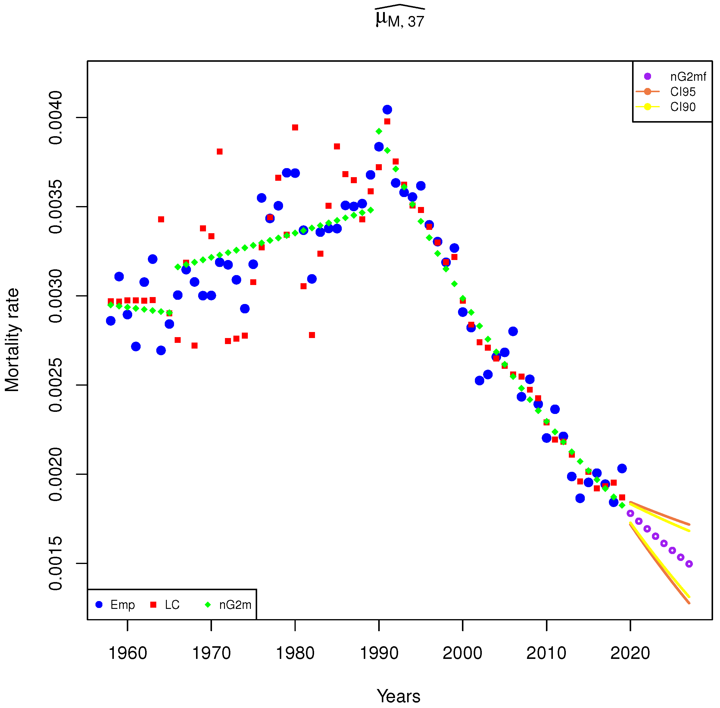
Figure 6.
The values of mortality rates—female, age 35: empirical (Emp), theoretical (LC, nGs), forecasts (nGsf), and c. interval based on the LC, and nGs model with switch.
Figure 6.
The values of mortality rates—female, age 35: empirical (Emp), theoretical (LC, nGs), forecasts (nGsf), and c. interval based on the LC, and nGs model with switch.

Figure 7.
The values of mortality rates—male, age 22: empirical (Emp), theoretical (LC, nGs), forecasts (nGsf), and c. interval based on the LC, and nGs model with switch.
Figure 7.
The values of mortality rates—male, age 22: empirical (Emp), theoretical (LC, nGs), forecasts (nGsf), and c. interval based on the LC, and nGs model with switch.


Table 1.
MSE (goodness of fit), F-statistics, p-value (pv)).
| Age | MSEEM-LC | MSEEM-nG | MSEEM-nGMs | ||
|---|---|---|---|---|---|
| 0.195 (0.02) | 8.69 (0.004) | ||||
| 0.22 (0.03) | 0.18 (0.02) | ||||
| 0.12 (0.01) | 5.15 (0.02) | ||||
| – | 0.27 (0.0197) | 192 () | |||
| – | – | – | |||
| – | – | – |
Table 2.
The 90% and 95% CI for the forecast of the mortality rates (2020–2027; L: left, R: right).
| CI | ||||||
|---|---|---|---|---|---|---|
| 90% L | 4.57 | |||||
| 90% R | ||||||
| 95% L | ||||||
| 95% R |
Publisher’s Note: MDPI stays neutral with regard to jurisdictional claims in published maps and institutional affiliations. |
© 2022 by the authors. Licensee MDPI, Basel, Switzerland. This article is an open access article distributed under the terms and conditions of the Creative Commons Attribution (CC BY) license (https://creativecommons.org/licenses/by/4.0/).
Share and Cite
MDPI and ACS Style
Sliwka, P.; Socha, L. Application of Continuous Non-Gaussian Mortality Models with Markov Switchings to Forecast Mortality Rates. Appl. Sci. 2022, 12, 6203. https://doi.org/10.3390/app12126203
AMA Style
Sliwka P, Socha L. Application of Continuous Non-Gaussian Mortality Models with Markov Switchings to Forecast Mortality Rates. Applied Sciences. 2022; 12(12):6203. https://doi.org/10.3390/app12126203
Chicago/Turabian StyleSliwka, Piotr, and Leslaw Socha. 2022. "Application of Continuous Non-Gaussian Mortality Models with Markov Switchings to Forecast Mortality Rates" Applied Sciences 12, no. 12: 6203. https://doi.org/10.3390/app12126203
Note that from the first issue of 2016, this journal uses article numbers instead of page numbers. See further details here.