Jointed Rock Failure Mechanism: A Method of Heterogeneous Grid Generation for DDARF

Abstract

The original DDARF (discontinuous deformation analysis for rock failure) can only generate uniform grids, and the increase in the number of grids reduces the efficiency of calculation, which limits the use of DDARF in large-scale geotechnical engineering. This is a problem that needs to be solved in the original DDARF. A new method is proposed in this paper to optimize the generation of grids in DDARF, and the optimized DDARF can generate heterogeneous grids. The model of the Brazilian disc-splitting experiment was established by using the optimized DDARF, fine grids were generated in the crack propagation region of the model, andsparse grids were generated at the edge of the model. The simulation results show that the Brazilian disc-splitting experiment simulated by the optimized DDARF is more consistent with the physical experiment than the original DDARF. The optimized DDARF and the original DDARF were used to generate a heterogeneous grid model and a uniform grid model, respectively, to simulate the uniaxial compression experiment. Through the analysis of the experimental results, it can be concluded that the optimized DDARF is more accurate in simulating the cracking and propagation of joints in rock blocks, the results of optimized DDARF are more consistent with the simulation results of other software, and the computational efficiency of the optimized DDARF simulation experiment is much higher than that of the original DDARF at the same time.

1. Introduction

A rock mass not only contains intact rock but also discontinuous structural planes. The rock mass mechanical properties are controlled by both the rock and the structural planes, often showing the characteristics of non-uniformity, discontinuity, anisotropy and multiple phases [1,2,3,4]. The existence of structural planes greatly weakens the mechanical properties and stability of a rock mass. The deformation and strength properties of discontinuity often play a controlling role in the deformation and stability of a rock mass [5,6,7]. A large number of facts show that the instability of geotechnical engineering takes the crack expansion inside a rock mass as the breakthrough point, causing large deformation and displacement of the rock mass and leading to the occurrence of disasters and accidents (p. 1, [8]). Consequently, it is very significant to research the initiation, propagation and connection of fissuring in rock mass to reveal the failure mechanism of rock masses and to evaluate the safety and reliability of geotechnical engineering (pp. 1–2, [8]), [9,10,11,12]. In practical engineering, it is difficult to obtain an analytical solution owing to the heterogeneity of rock mass, the nonlinear constitutive relationship of rock mass, the discontinuity caused by discontinuities of rock mass and the complexity of boundary conditions, and the approximate solution can only be obtained by numerical analysis (pp. 206–208, [13]), therefore, numerical simulation and digital rock technology are playing increasingly important roles in the study of rock properties, and many scholars have obtained important conclusions by using these methods [14,15,16,17].

The deformation and failure of rock masses occur through discontinuous deformation. A discontinuous numerical method—discontinuous deformation analysis (DDA)—which can fully consider the discontinuity of a rock mass has been proposed and can be used to simulate the discontinuous deformation and large displacement motion of massive rock masses [18,19]. Based on the DDA method, an analysis method for the failure process of discontinuous jointed rock masses—discontinuous deformation analysis for rock failure (DDARF)—has been constructed and can be used to simulate the entire process of crack initiation, expansion, convergence and connection in jointed rock masses, opening up a new way to simulate the entire failure process of rock masses (p. 132, [8]), [11,20].

In numerical simulation, as the number of grids in the model increases, the accuracy of calculation increases, but the efficiency of calculation decreases [9,21,22,23,24]. However, the DDARF program can only generate uniform grids in the process of establishing the model. In order to achieve the calculation accuracy requirements, DDARF needs to generate a large number of grids, which not only increases the amount of calculation required but also reduces computational efficiency and can even sometimes lead to the failure of the calculations. These characteristics of DDARF limit its use in large-scale geotechnical engineering [25,26]. In order to balance the accuracy and efficiency of calculation, the authors optimized the grid generation of DDARF so that it could generate heterogeneous grids; dense grids were generated at the preset joints, and sparse grids were generated far away from the preset joints, which not only ensured the accuracy of calculation but also improved the efficiency of calculation.

The DDARF method is based on the improved DDA method, which is used to solve the failure problem of the discontinuous jointed rock mass. In this method, the computational region is automatically divided into triangular block elements by the traveling wave method, and the block boundary is divided into the real joint boundary and virtual joint boundary. For all joints in the model, they are defined as virtual joints when they fail to reach the fracture failure criterion. After the strength reaches the fracture failure criterion in the calculation process, they are transformed into real joints to form cracks, and the real joint strength parameters are assigned to them. The crack propagation is carried out along the virtual joints and in accordance with the criterion of interfacial fracture. The deformation and failure process of discontinuous joints can be considered as the cracking, expansion and penetration of virtual joints. In this process, the mechanical properties of virtual joints (cohesion, internal friction angle, tensile strength) are weakened and the overall strength of discontinuous joints is reduced. Therefore, the DDARF method can simulate the whole process of crack initiation, propagation, penetration and rock fragmentation and can be applied to complete rock, discontinuous jointed rock mass and even completely discontinuous rock mass and other phenomena [8,11,20,25].

There are several calculation theories involved in DDARF, which have been described as follows (pp. 25–41, 63–65, [8]):

1.1. Automatic Generation of Random Joint Networks

In order to simulate random joints in the DDARF method, an automatic generation algorithm of random joints network is proposed. The Monte Carlo method is used to generate (0,1) uniformly distributed random numbers, and then these random numbers are used to generate other random numbers subject to some distributions. Therefore, the geometric parameters of the joints can be generated randomly, including center position, direction angle and length. Thus, the specific location of each joint in space can be determined so that their spatial distribution satisfies the given distribution law. In this program, it is assumed that the center position of joints obeys a uniform distribution, and the direction angle and length obey the normal distribution (p. 25, [8]).

1.2. Automatic Generation of Triangular Block Grid

The DDARF program uses the automatic generation technique of the computational grid traveling wave method to discretize the computational area into a fine triangular block system. First, it adds virtual joints to the isolated endpoints and divides the complex computing domain into several simply connected subdomains with simple shapes. Then, it combines the meshes of each subdomain together to generate meshes in each simply connected subdomain. In this way, the meshes of the computing domain are generated (pp. 25–26, [8]).

1.3. Analysis of Block Boundary Cracking

The discontinuous jointed rock mass is discretized into fine triangular block grids by the block automatic generation algorithm. The boundary of the triangular block grids, the virtual joints, provides a path for crack propagation. The triangular block grids on both sides of the virtual joints are bonded by the sticky settlement method. If the two grids are in contact, they need to add normal and tangential contact springs to prevent normal insertion and tangential slip. If the contact spring force exceeds the joint strength, the contact springs are removed and the two grids can move separately. Therefore, the restraint of the spring can be maintained by increasing the joint strength parameters so that the two grids are bonded together. It is based on this idea that the strength parameters of virtual joints are increased to achieve bonding between grids. If the relative displacement of the grids on both sides of the virtual joint is too large, and the contact force of the spring reaches the strength of the rock, the contact spring is destroyed, and the virtual joint becomes a real joint to form a crack, and the real joint strength parameters are assigned to it. In this way, the simulation of crack propagation is realized.

The failure of the contact spring is judged by two criteria: normal tension failure and tangential compression–shear failure. The failure criterion of a normal spring is that when the maximum tensile principal stress reaches a given value, the spring fails. The tangential compression–shear failure criterion considers that when the spring meets the Mohr–Coulomb criterion, the spring fails. At the same time, the tensile failure criterion has priority. If the tensile failure criterion is satisfied, it is not necessary to judge whether the compression–shear failure criterion is satisfied. Only if the tensile criterion is not satisfied can the compression–shear failure criterion be determined. The normal spring tensile failure criterion is as follows:

$${\mathrm{f}}_{\mathrm{n}}=-{\mathrm{T}}_0\mathrm{l}$$

(1)

The tangential spring compression-shear failure criterion is as follows:

$${\mathrm{f}}_{\mathsf{\tau }}=\mathrm{c}\mathrm{l}+{\mathrm{f}}_{\mathrm{n}}\tan \mathsf{\phi }$$

(2)

Terms in the equation: ${\mathrm{f}}_{\mathrm{n}}$—Normal contact force; ${\mathrm{f}}_{\mathsf{\tau }}$—Tangential contact force; ${\mathrm{T}}_0$—Uniaxial tensile strength of the rock; $\mathrm{c}$—Cohesion of the rock; $\mathsf{\phi }$—Friction angle of the rock; and $\mathrm{l}$—Length of contact.

According to the contact force and failure criteria calculated by Equations (1) and (2), it can be judged as to whether the contact spring is damaged or not. If it is damaged, the virtual joint becomes the real one and its strength decreases to the strength of the real one (pp. 40–41, [8]).

1.4. Simulated Material Inhomogeneity

The Weibull distribution is used for the mechanical parameters of the triangular grid blocks to simulate the inhomogeneity of the rock mass, and the probability density function of the Weibull distribution can be expressed as:

$$\mathsf{\phi }(\mathrm{h},\mathsf{\beta })=\frac{\mathrm{h}}{{\mathsf{\beta }}_0}{(\frac{\mathsf{\beta }}{{\mathsf{\beta }}_0})}^{\mathrm{h}-1}{\mathrm{e}}^{-{(\frac{\mathsf{\beta }}{{\mathsf{\beta }}_0})}^{\mathrm{h}}}$$

(3)

where, $\mathsf{\beta }$—The value of a certain mechanical parameter, such as modulus of elasticity, Poisson’s ratio; ${\mathsf{\beta }}_0$—The average value of the parameter; $\mathrm{h}$—Homogeneity rate or homogeneity coefficient, which characterizes the homogeneity of the material. The greater its value, the more homogeneous the material is, and $\mathrm{h}\ge 1.0.$

By integrating Equation (3), we can obtainthe Weibull distribution function as follows:

$$\mathsf{\Phi }(\mathrm{h},\mathsf{\beta })=1-{\mathrm{e}}^{-{(\frac{\mathsf{\beta }}{{\mathsf{\beta }}_0})}^{\mathrm{h}}}$$

(4)

The linear congruence method is used to generate n random numbers, ξ_i, in the interval [0, 1], the general recursive equation of linear congruence method is:

$$\{\begin{array}{l}{\mathrm{x}}_{\mathrm{n}}=(\mathrm{a}{\mathrm{x}}_{\mathrm{n}-1}+\mathrm{c})(\mathrm{mod}\mathrm{M})\\ {\mathrm{r}}_{\mathrm{n}}=\frac{{\mathrm{x}}_{\mathrm{n}}}{\mathrm{M}}\\ \mathrm{Initial}\mathrm{Value}{\mathrm{x}}_0\end{array}$$

(5)

Terms in the equation: $\mathrm{M}$—Module; $\mathrm{mod}\mathrm{M}$—Mod the module M; $\mathrm{a}$—The multiplier; $\mathrm{c}$—Incremental; ${\mathrm{x}}_0$—The initial value; ${\mathrm{r}}_{\mathrm{n}}$—A random number evenly distributed in the interval [0, 1]; the above parameters $\mathrm{M}$,$\mathrm{a}$,$\mathrm{c}$, and ${\mathrm{x}}_0$ should follow the following criteria, given by Kunth:

(1)

${\mathrm{x}}_0$ is any non-negative integer;

(2)

$\mathrm{a}$ meets: $\mathrm{a}(\mathrm{mod}8)\equiv 5,\frac{\mathrm{M}}{100}<\mathrm{a}<\mathrm{M}-\sqrt{\mathrm{M}}$

(3)

$\mathrm{c}$ is odd, and $\frac{\mathrm{c}}{\mathrm{M}}=\frac{1}{2}-\frac{\sqrt{3}}{6}\approx 0.211324865$

According to previous experience, the parameters in this program are: $\mathrm{a}=2053, \mathrm{c}=13849, \mathrm{M}=65536, {\mathrm{x}}_0$ is the time function time (). These random numbers distribute uniformly in the [0, 1] interval, and then the direct sampling method is used in Equation (6) to obtain n Weibull distribution elastic modulus η_i, which are assigned to the n blocks; Poisson’s ratios of these n grid blocks are obtained in the same way (pp. 26, 63–65, [8]).

$$\begin{array}{l}\mathsf{\Phi }({\mathsf{\eta }}_{\mathrm{i}})={\mathsf{\xi }}_{\mathrm{i}}\\ {\mathsf{\eta }}_{\mathrm{i}}={\mathsf{\beta }}_0{[-\ln (1-{\mathsf{\xi }}_{\mathrm{i}})]}^{\frac{1}{\mathrm{h}}}\end{array}$$

(6)

2. The Methodology of Heterogeneous Grid Generation for DDARF

In order to improve the accuracy of simulation calculation, fine grids need to be generated in the model, but the original DDARF can only generate a uniform grid. In order to satisfy the calculation accuracy, fine grids are generated in the whole model, which increases the calculating workload and time and is not realistic for use in large-scale geotechnical engineering. In order to solve this problem, a method to generate heterogeneousgrids is proposed in this paper.

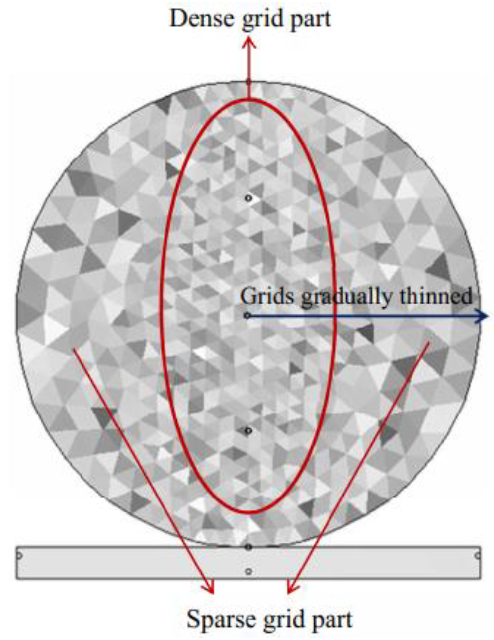
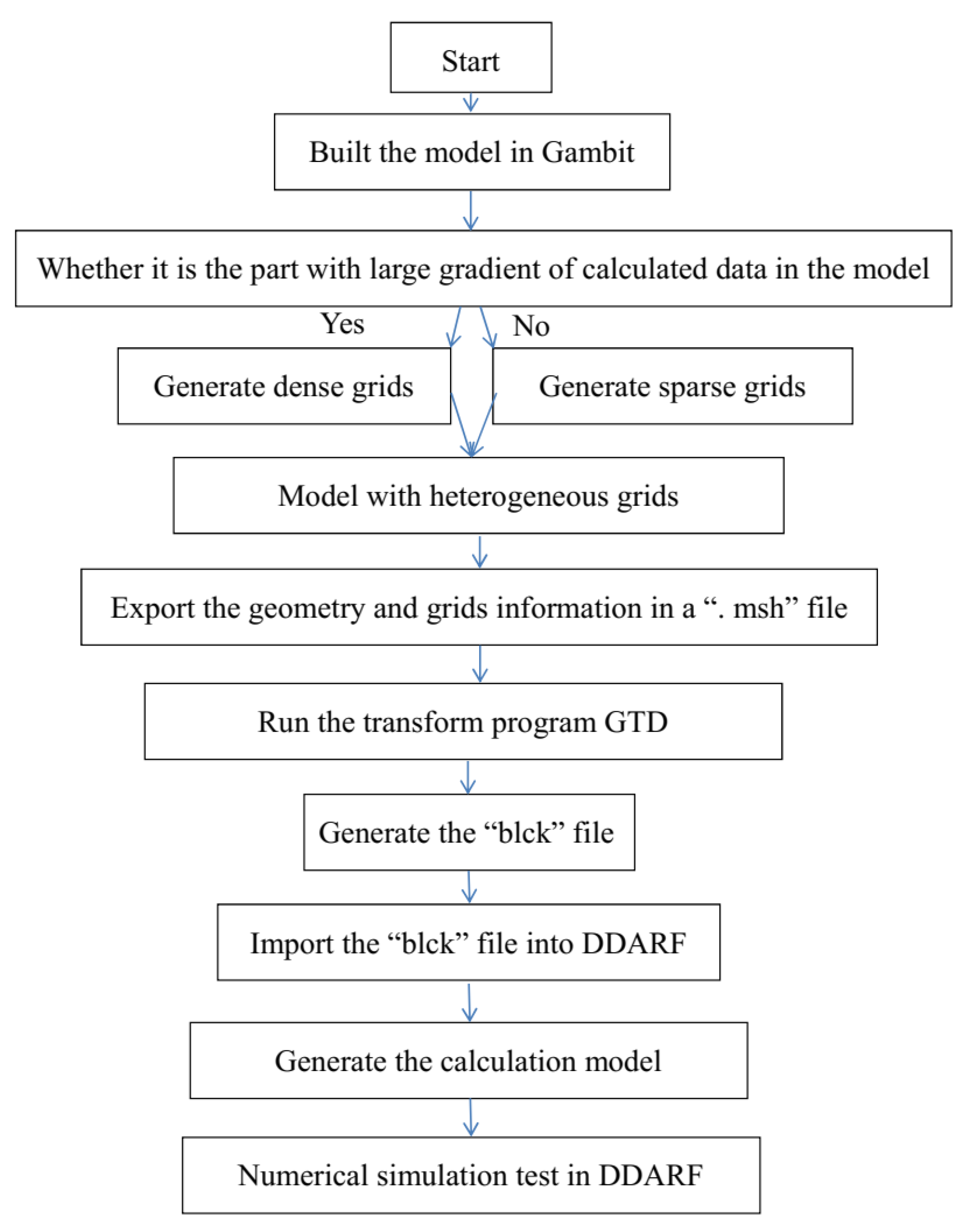
2.1. Gambit Modeling and Generation of Heterogeneous Grids

Gambit is a kind of mesh generation software from Fluent. Its main functions include geometric modeling and mesh generation. Gambit is mainly used as the mesh generation software of Fluent software, also known as the specialized mesh generation software of Fluent [27].

Firstly, the model is built in Gambit and heterogeneous grids are generated. During the grid generation process, dense grids can be generated in some parts as needed and sparse grids can be generated in the other parts of the model, according to the calculation requirements, as shown in Figure 1.

2.2. Transform Program GTD (Gambit to DDARF)

When DDARF performs numerical simulation calculation, all models and grid information are stored in a “BLCK” file in a certain format. However, the grid information in the “.msh” file exported from Gambit is inconsistent with the format of the “BLCK” file and cannot be directly imported into DDARF for use, so the transform program GTD is written in the python language. Through GTD, data with the heterogeneous grid model generated by Gambit can be imported into DDARF to generate a heterogeneous grid model, as shown in Figure 2.

The technical flowchart of the heterogeneous grid generation in DDARF is shown in Figure 3.

3. Results and Discussion

3.1. Accuracy Verification of the Optimized DDARF Program

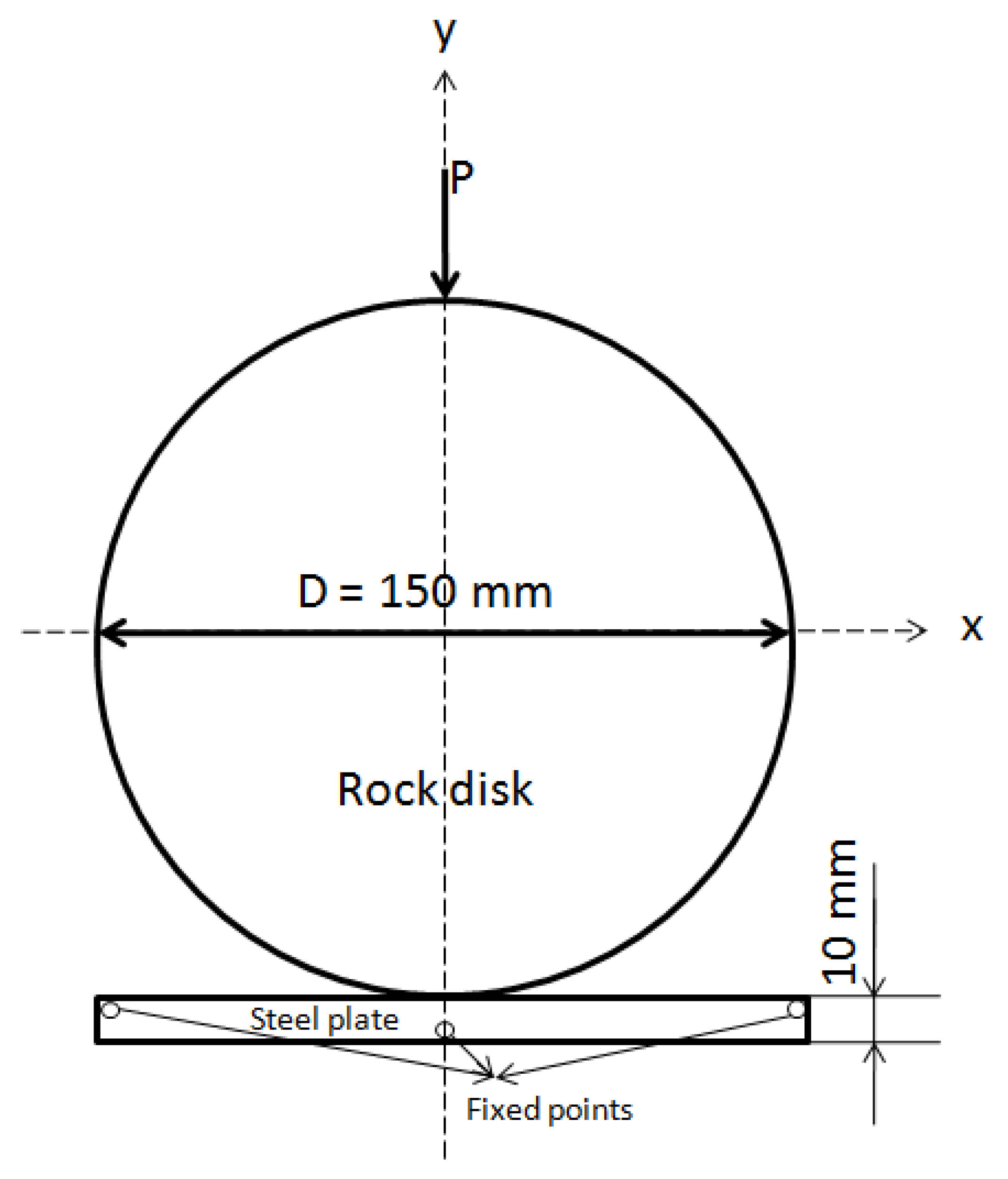
3.1.1. Model Parameters and Loading Mode

This experiment simulates the Brazilian disc-splitting experiment; the model geometric parameters and loading mode of the simulation experiment are shown in Figure 4. The model diameter of the Brazil disc is 150 mm, and a 10 mm-thick steel plate is added to the lower part of the model. The steel plate is fixed with three fixed points. The top of the disc is loaded with concentrated force P.

The boundary conditions are as follows: a steel plate is placed at the bottom of the Brazilian disc, the steel plate is fixed, and a concentrated force P is applied at the top of the Brazilian disc, which linearly and slowly increases from 0 until the calculation finished and the other parts of the Brazilian disc are free.

Mechanical parameters of the Brazilian disc model are shown in

Table 1. Mechanical parameters of the Brazilian disc model.

Density (kg/m3)	Elastic Modulus (GPa)	Elastic Modulus Uniformity Coefficient	Poisson’s Ratio	Poisson’s Ratio Uniformity Coefficient	Friction Angle (°)	Cohesion (MPa)	Tensile Strength (MPa)
2500	70	15	0.3	100	30	40	15

: the elastic modulus of the lower steel plate is 100 GPa and the Poisson’s ratio of the steel plate is 0.3.

The optimized DDARF program is used for modeling and calculation. In order to observe the initiation, expansion and penetration of splitting cracks, the grids in the middle part of the Brazilian disc model are dense, while the sparse grid is still used on both sides of the model to improve the calculation efficiency, as shown in Figure 2. A concentrated force, P, was applied to the top of the Brazilian disc model, and its value increased linearly from 0. With the increase in P, the failure process of the Brazilian disc model could be observed, as shown in Figure 5. The convergence condition of the calculation is that the displacement generated in one step is less than 0.001 of the displacement generated in the previous step, which is convergence [11].

3.1.2. Analysis and Comparison of Results

After loading, vertical main cracks appeared firstly in the top and bottom of the model, as shown in Figure 5b;with the load continuing, some secondary cracks appeared next to the main cracks which were at the top and the bottom of the model, as shown in Figure 5c, which is consistent with Zhang Xiuli’s research (pp. 60–61, [28]). As the load continued to increase, the vertical main cracks which first appeared continued to expand vertically (Figure 5d), and finally the vertical main cracks broke through, resulting in the destruction of the model (Figure 5e).

Figure 6 is the physical experiment of the Brazilian disc-splitting experiment (pp. 80–82, [8]). It can be seen that, after the experiment, a crack appears in the middle of the disc, which divides the disc into two parts; the failure characteristics of the physical experiment are consistent with those of the Brazilian disc-splitting experiment simulated by the optimized DDARF, which verifies the effectiveness of the optimized DDARF in rock simulations. To compare with the results of the Brazilian disc-splitting experiments simulated in the original DDARF by ZhangXiuli (p. 61, [28]) as shown in Figure 7, it can be seen that the destruction of the model law is consistent, and because the optimized DDARF program defined the grid density of crack initiation and expansion area, it can simulate more subtle crack initiation in the splitting process of the Brazilian disc, as shown in Figure 5e.

3.2. Superiority Verification of the Optimized DDARF Program

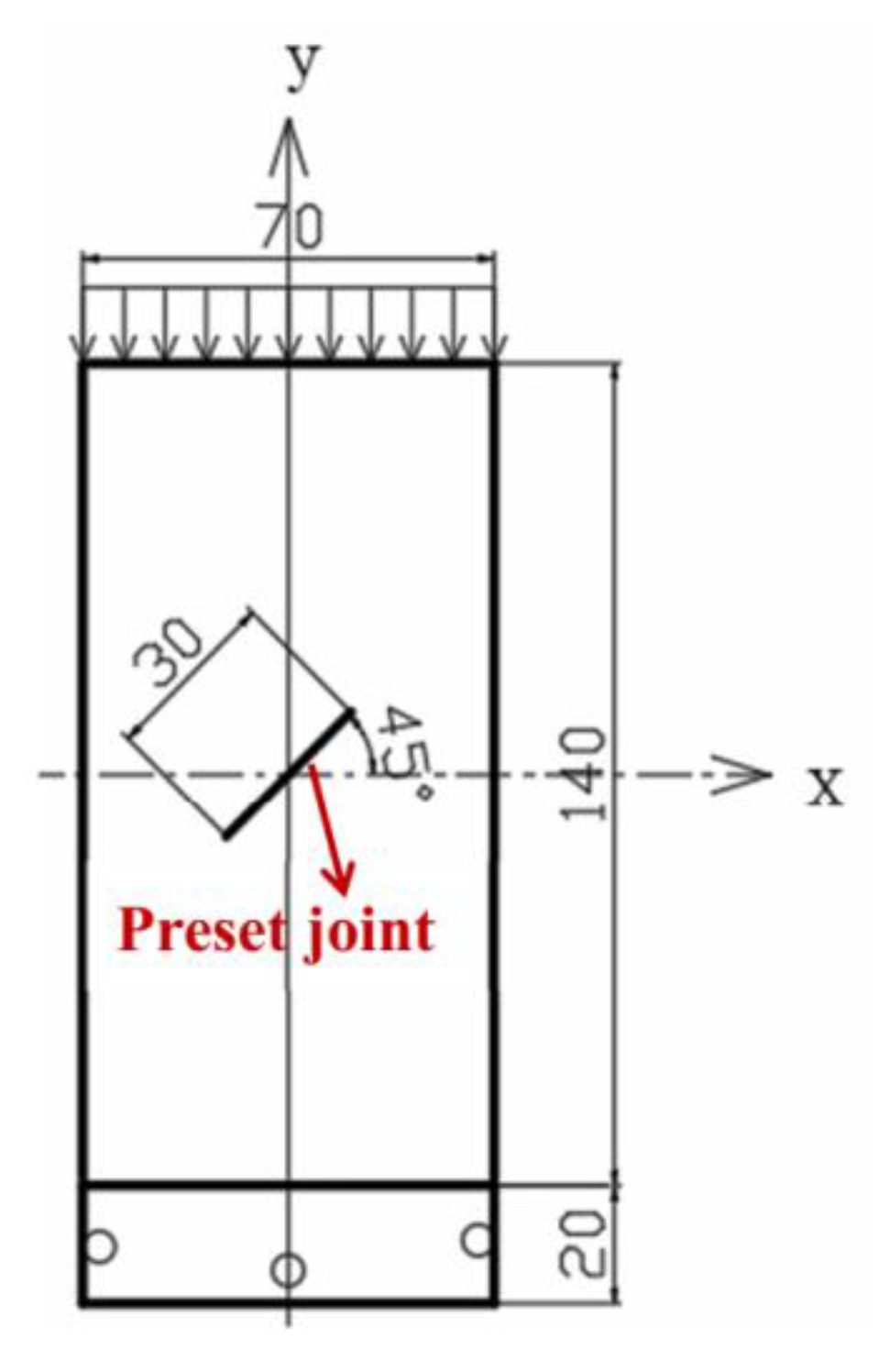
3.2.1. Model Building and Loading Mode

In order to research the advantages of the optimized DDARF in grid generation, calculation accuracy and calculation efficiency, uniaxial compression experiments were simulated by the optimized DDARF and original DDARF. The fracture opening of rock has self-similarity, and its analysis can be conducted by using fractal theory, which can simulate the expansion law of joints in rock mass. Some scholars have also obtained important conclusions through fractal modeling [29]. Based on fractal theory, the following models can be established.

Three cases of rock models are established: Case 1, Case 2 and Case 3. The geometric parameters of the rock models in the three cases are shown in Figure 8. The dimensions of the rock models in the three cases are 140 mm × 70 mm. A steel plate with a thickness of 20 mm is added to the bottom for fixing, and there is a preset joint with a length of 30 mm in the middle of the rock model. The mechanical parameters of the rock models are shown in

Table 2. Mechanical parameters of the rock models.

Density (kg/m3)	Elastic Modulus (GPa)	Elastic Modulus Uniformity Coefficient	Poisson’s Ratio	Poisson’s Ratio Uniformity Coefficient	Friction Angle (°)	Cohesion (MPa)	Tensile Strength (MPa)
2310	10	15	0.25	20	30	40	25

, the elastic modulus of the lower steel plate is 100 GPa, and the Poisson’s ratio of the steel plate is 0.25. A total of eight measuring points are set in the upper, middle and lower parts of the model, which can record the stress and displacement during calculation.

The boundary conditions of the uniaxial compression experiment are as follows: a steel plate is placed at the bottom of the rock block, the steel plate is fixed, a uniform load is applied on the upper part of the rock block, and the value of the uniform load increases slowly from 0 until the calculation finished and the remaining parts of the rock block are free.

In Case 1, the original DDARF program is used to generate the grid, as shown in Figure 9a. The grids are uniform with a total of 817. After calculation, the area of each grid is about 12 mm².

Case 2 uses the optimized DDARF program for grid generation, as shown in Figure 9b, in order to observe the expansion of the preset joint. Dense grids are generated in the area around the preset joint, while in the area away from the preset joint sparse grids are generated, and the total number of grids is also 817. The area of each dense grid is around in 1–5 mm² while that of each sparse grid area is about 40 mm²–50 mm².

In Case 3, the original DDARF is used for grid generation. In order to compare the calculation accuracy, the area of each grid in this case is also about 1 mm²–5 mm²; however, since the original DDARF can only generate uniform grids, an average area value of 3 mm² is taken as the area of each grid. Thus, there should be 3267 grids generated and a uniform grid model with 3267 grids, as shown in Figure 9c.

A uniformly distributed load is applied above the model, as shown in Figure 8,to conduct a numerical simulation experiment of uniaxial compression. Screen recording software is used to record the whole process.

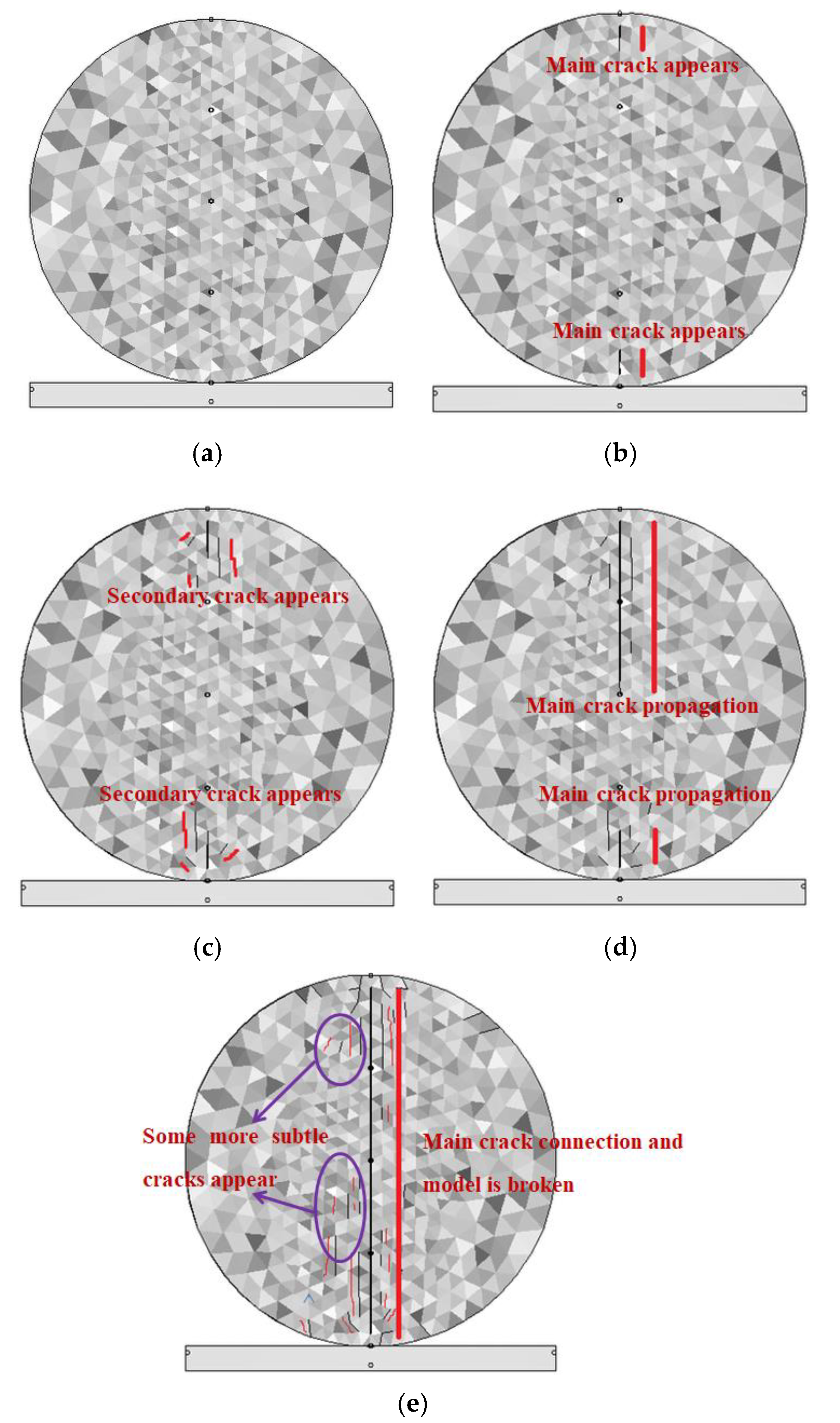
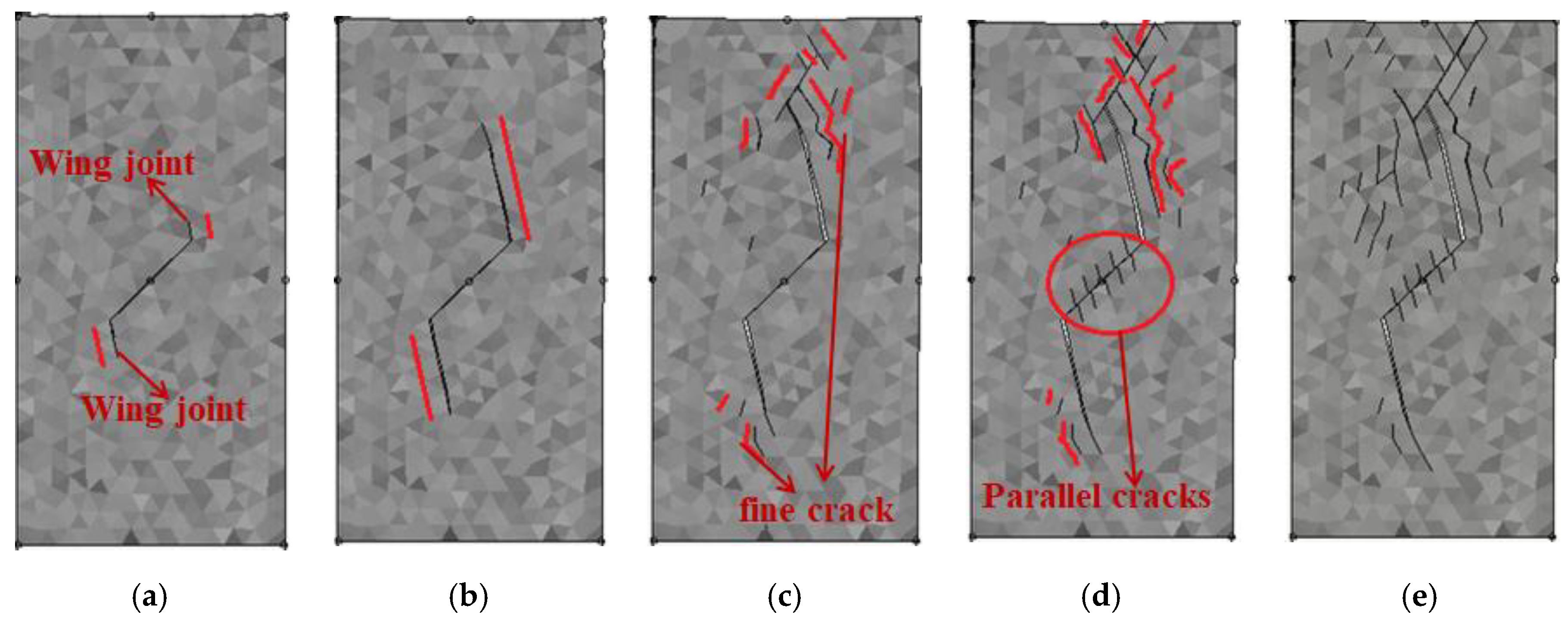
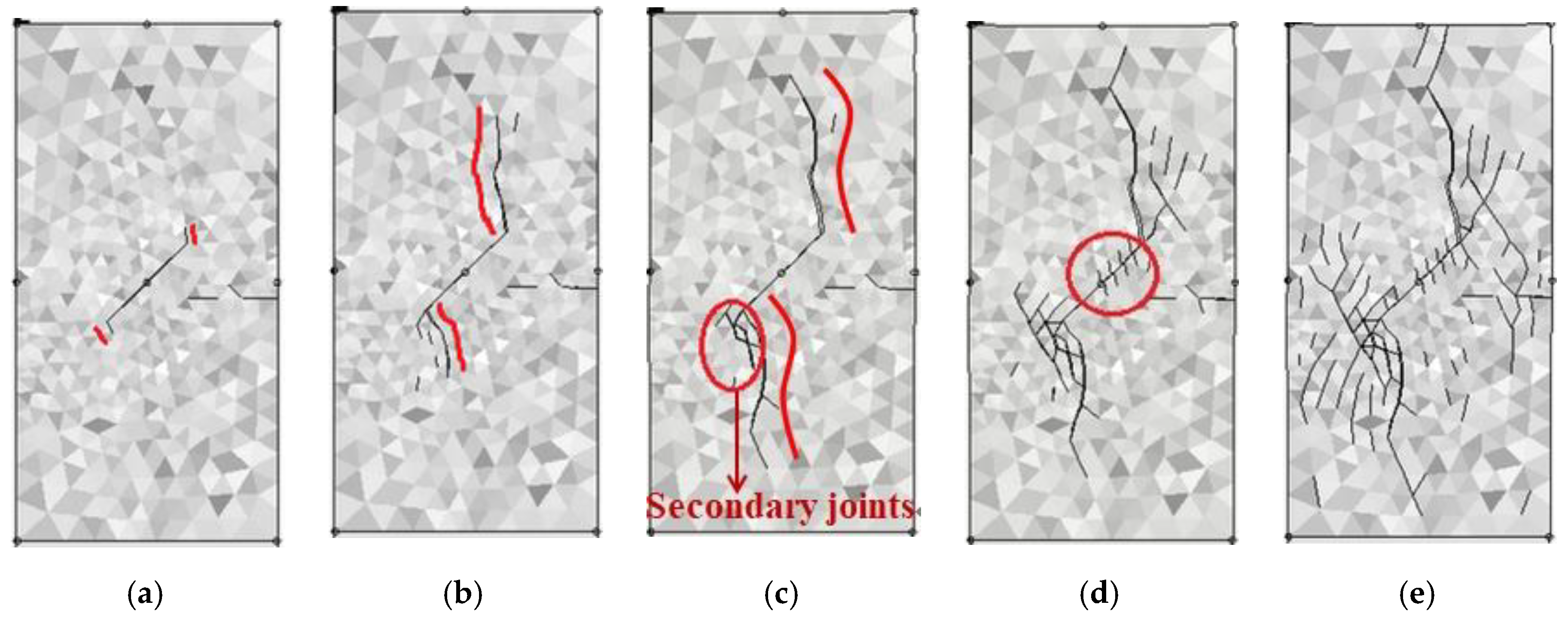
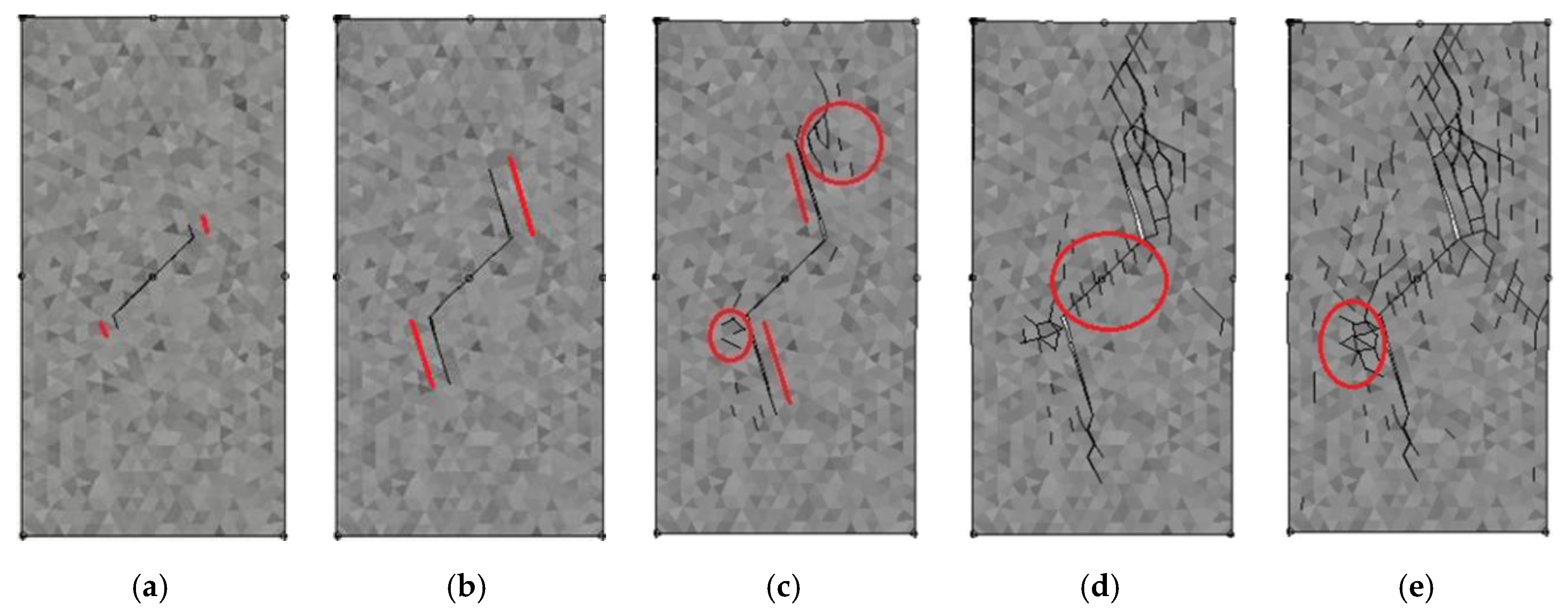
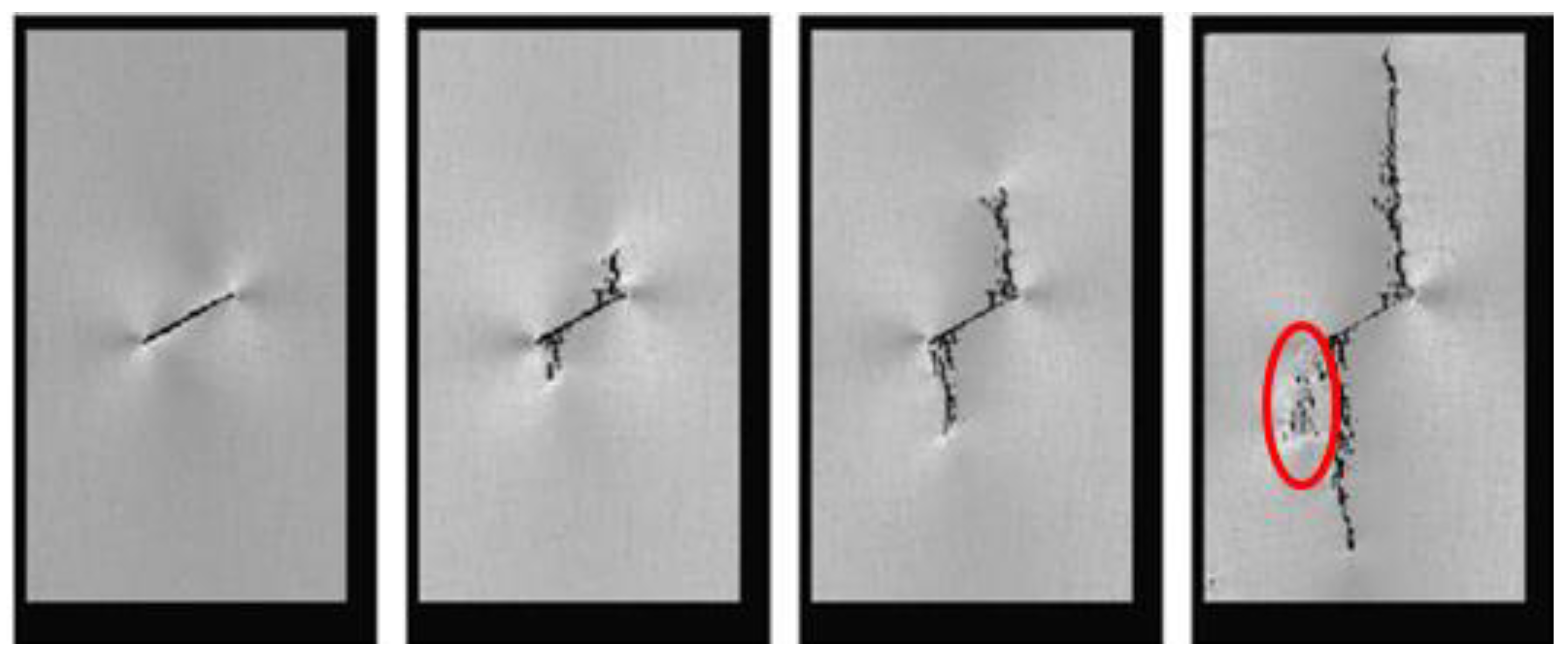
3.2.2. Analysis of Model Cracking Process

In the experimental process, the models of the three cases showed similar rules: after loading, the models first demonstrated compression deformation, and the preset joints display compaction. With the progress of compression, the ends of the preset joints cracked, and wing cracks appeared (Figure 10a, Figure 11a and Figure 12a). The wing cracks expanded in the direction of the large principal stress (Figure 10b, Figure 11b and Figure 12b). The width of the wing crack increased with the load increase (Figure 10c, Figure 11c and Figure 12c). The propagation of the upper wing cracks extended in the axial direction through the top of the model; a group of new oblique parallel cracks appeared on the preset joints (Figure 10d, Figure 11d, and Figure 12d). At the same time, some fine cracks appeared in the model, which expanded with the increase in pressure, and the fine cracks became connected with the wing cracks and preset joints (Figure 10e, Figure 11e and Figure 12e), which finally led to the failure of the model. The above analysis shows that the optimized DDARF program can effectively simulate the uniaxial compression experiment of rock blocks.

However, there are some subtle differences among the three models in the expansion of the joint, as follows: in the process of the expansion of the preset joint, after the wing cracks appeared at the ends of the preset joints of the Case 1 model, wing cracks expanded along the axis and secondary joints did not appear near the ends of the preset joint, as shown in Figure 10b–e. In the model of Case 2, after the wing cracks appeared at the end of the preset joint, some secondary joints appeared near the left end of the preset joint during the expansion of the wing cracks. The increase and expansion of secondary joints resulted in the fragmentation of the rock mass at the left end of the preset joint, as shown in Figure 11c–e. This failure rule is consistent with the numerical simulation results of other scholars, as shown in Figure 13 [30]. The reason for these kinds of failure rules is that the grids generated near the preset joints in Case 2 are relatively dense and can show more subtle changes. In the model of Case 3, secondary joints also appear at the left end of preset joints in the process of wing crack propagation, resulting in the fragmentation of rock mass in this part, as shown in Figure 12c–e, indicating that the accuracy of simulating rock block failure in Case 2 is close to that in Case 3.

In short, the failure process of rocks can be more carefully simulated in Case 2 than in Case 1, and the results are closer to those of other scholars. The joint expansion law of Case 2 in the dense grid region is close to that of the Case 3 model with a large number of uniform grids. The above analysis shows that the optimized DDARF has advantages in simulating the law of joint expansion.

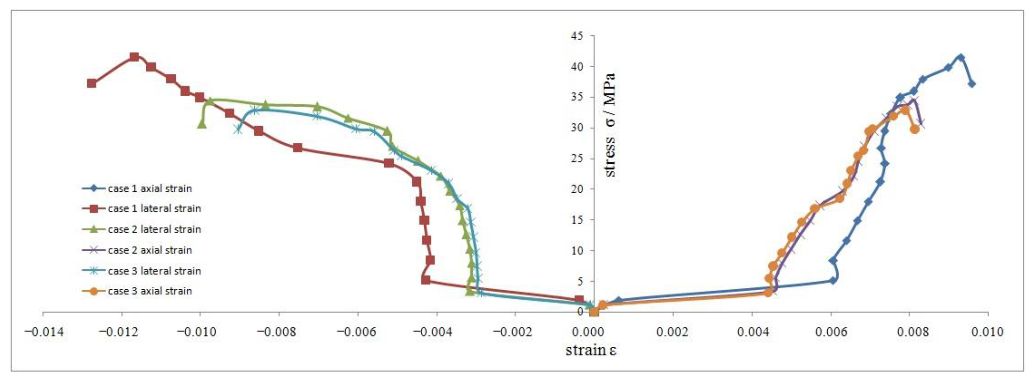
3.2.3. Stress Comparison

Eight measuring points are set at the top, left and right sides of the border of the three case models to measure the displacements and stresses of the models in the compression simulation experiments, after the simulation, according to the measured values of the measuring points.Stress–strain curves of the three cases models can be obtained, as shown in Figure 14 (taking compression as positive and tension as negative).

As can be seen from the curves in Figure 14, the three cases all experienced three stages in the experimental process of the model:

1.

Compaction stage

The preset joints in the models displayed closed compaction, and the whole models are axially compressed and laterally expanded, so the axial strain was positive strain (axial compression) and the lateral strain was negative strain (lateral expansion) on the stress–strain curve.

2.

Elastic deformation stage

In this stage, the curves showed linear growth, the axial and lateral strains continued to increase, and the slope increased compared with the compaction stage. Near the end of this stage, the preset joint began to crack.

3.

Steady crack growth stage

The main cracks continued to expand, and secondary cracks appeared in other parts of the models. The slope of the curve changed a lot in this stage, mainly caused by the increase in the number of cracks in the model. After the stress reached the peak, the curves began to decline, indicating that the models were damaged. At the end of the experiment, the lateral strains of the models under the three cases were greater than the axial strains, indicating the dilatation phenomenon of the models.

Although the stress–strain curves of the three cases vary in the same way, the stress at the initiation of preset joints (crack initiation stress) and the maximum stress (peak stress) of the three cases were both different; crack initiation stress and peak stress are very important for the study of mechanical properties of rock mass with joints [31,32,33,34]. The crack initiation stress and peak stress in the three cases are shown in

Table 3. Crack initiation stress and peak stress of the three cases.

Case	Crack Initiation Stress (MPa)	Peak Stress (MPa)	Crack Initiation Stress/Peak Stress (%)
1	21.19	41.56	50.99%
2	17.36	34.43	50.42%
3	16.84	32.87	51.23%

:

From Table 3, the crack initiation stress and peak stress of Case 1 are both the largest among the three cases, while the crack initiation stress of Case 2 and Case 3 is similar, as is the peak stress, which shows that the calculation accuracy of Case 2 and Case 3 is approximately the same, suggesting that the optimized DDARF’s calculation accuracy in the simulation experiment is in agreement with the model with the greater number of fine uniform grids (Case 3).

According to the cracking algorithm principle of the DDARF, virtual joints provide channels for the expansion of the joints and cracks—that is to say, the more virtual joints there are, the more joints expand where they are supposed to expand. In Case 1, due to the small number of grids and large area of each grid, the cracking and expansion of the joints are hindered, and the crack initiation stress and peak stress of joints are relatively large. On the other hand, in the DDARF, after the triangular grids are generated, if two grid blocks are in contact, the normal and tangential contact springs are added between them to restrain normal embedding and tangential slip. If the contact spring force exceeds the virtual joint strength, the contact spring is damaged and removed, the two grid blocks can move independently and the virtual joint becomes the real joint. According to the calculated contact force and failure criteria in Equations (1) and (2), whether the contact spring is damaged can be determined. From Equations (1) and (2), it can be seen that, with two adjacent triangle grid blocks, the contact length $\mathrm{l}$ is greater, the failure criterion values ${\mathrm{f}}_{\mathrm{n}}$ and ${\mathrm{f}}_{\mathsf{\tau }}$ are higher, the spring is less easily damaged and the virtual joint less easily becomes a real joint—that is, the stress is higher when there is a real joint in the rock, which leads to higher crack initiation stress and peak stress.

3.2.4. Computing Efficiency Comparison

In the calculation of the DDARF, screen recording software is used to record the whole process, and the time spent in the simulation experiment of each case can be recorded, as shown in

Table 4. Calculation time statistics of three cases.

Case	Crack Initiation Time	Failure Time
1	1:14	8:45
2	1:35	8:33
3	2:27	17:46

.

According to Table 4, in the Case 1 and Case 2 models, the preset joints initiate in more than one minute, and before nine minutes, both casemodels are damaged. However, in the Case 3 model, the preset joint initiates at 2:27, and it takes as long as 17:46 for the model to be damaged. Therefore, the computational efficiencies of Case 1 and Case 2 are higher than that of Case 3, which indicates that for the same model, when the model grids are denser, the computational efficiency is lower. Compared with Case 2 and Case 3 with the same accuracy, the calculation time of Case 2 is about 50% shorter than that of Case 3; therefore, Case 2 can not only ensure the accuracy of the simulation calculation but also improve the efficiency of the calculation.

4. Conclusions

Through the data and comparison of the above simulation experiments, the following conclusions can be obtained:

• The optimization method proposed in this paper can effectively generate heterogeneous grids in DDARF, which solves the problem that the original DDARF could only generate uniform grids and overcomes the problem that the number of model grids in DDARF simulations for geotechnical engineering processes is too large to be calculated.
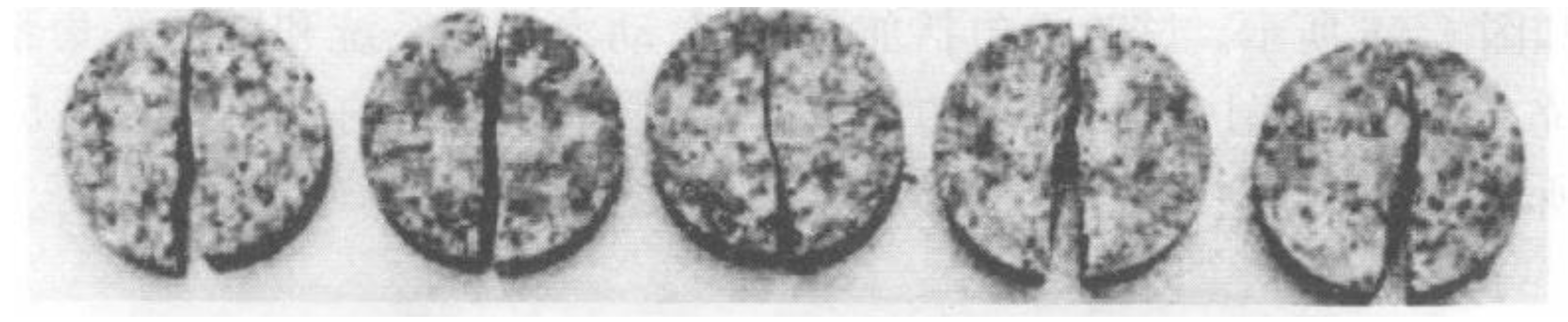
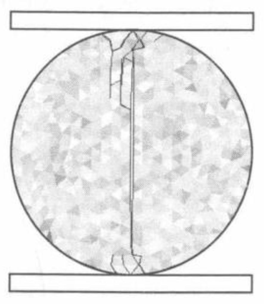
• The Brazilian splitting experiment can be simulated effectively by using the optimized DDARF program. Compared with the original DDARF program, the simulation results are more consistent with the physical experiment results.
• The optimized DDARF program was used to simulate the uniaxial compression experiment of rock blocks. Compared with the original DDARF program, it is more accurate in the cracking and expansion of joints and more consistent with the simulation results of the other software. At the same time, it can improve the calculation efficiency—that is to say, the optimized DDARF program has advantages in calculation accuracy and efficiency.

References

1. Liu, Y.; Tang, H. Rock Mass Mechanics; Chemical Industrial Press: Beijing, China, 2008; pp. 9–10. (In Chinese) [Google Scholar]
2. He, P.; Li, S.C.; Li, L.P.; Zhang, Q.Q.; Xu, F.; Chen, Y.J. Discontinuous Deformation Analysis of Super Section Tunnel Surrounding Rock Stability Based on Joint Distribution Simulation. Comput. Geotech. 2017, 91, 218–229. [Google Scholar] [CrossRef]
3. Wang, P.; Liu, C.; Qi, Z.; Liu, Z.; Cai, M. A Rough Discrete Fracture Network Model for Geometrical Modeling of Jointed Rock Masses and the Anisotropic Behaviour. Appl. Sci. 2022, 12, 1720. [Google Scholar] [CrossRef]
4. Pavičić, I.; Galić, I.; Kucelj, M.; Dragičević, I. Fracture System and Rock-Mass Characterization by Borehole Camera Surveying: Application in Dimension Stone Investigations in Geologically Complex Structures. Appl. Sci. 2021, 11, 764. [Google Scholar] [CrossRef]
5. Yan, C.; Xu, J.; Bao, H. Rock Mass Mechanics; People’s Communications Publishing House Co., Ltd.: Beijing, China, 2017; pp. 49–50. (In Chinese) [Google Scholar]
6. Dong, Z.; Hong, W.J.; Qian, Y.; Yi, J.Z.; Xiang, L.T. Experimental Study on Mechanical Characteristics of Sandstone Containing Arc Fissures. Arab. J. Geosci. 2018, 11, 637. [Google Scholar]
7. Liu, X.; Liang, Z.; Meng, S.; Tang, C.; Tao, J. Numerical Simulation Study of Brittle Rock Materials from Micro to Macro Scales Using Digital Image Processing and Parallel Computing. Appl. Sci. 2022, 12, 3864. [Google Scholar] [CrossRef]
8. Jiao, Y.; Zhang, X.; Li, T. DDARF Method to Simulate the Whole Process of Jointed Rock Mass Failure; Science Press: Beijing, China, 2009; pp. 1, 29–40, 63–66, 80–82. (In Chinese) [Google Scholar]
9. Zhu, W.S.; Chen, Y.J.; Li, S.C.; Yin, F.Q.; Yu, S.; Li, Y. Rock Failure and its Jointed Surrounding Rocks: A Multi-scale Grid Meshing Method for DDARF. Tunn. Undergr. Space Technol. 2014, 43, 370–376. [Google Scholar] [CrossRef]
10. Gao, Z.; Luo, J.; Wu, X.; Li, K. Deformation Analysis of the Rock Surrounding a Tunnel Excavated through a Gently Dipping Bed. Appl. Sci. 2022, 12, 1960. [Google Scholar] [CrossRef]
11. Wang, W.; Liu, G.W.; Su, Q.; Han, R. Analysis of Excavation Procedure and Stability in Jointed Rock Masses of the Large Underground Caverns. In Application of Intelligent Systems in Multi-modal Information Analytics; MMIA 2019; Advances in Intelligent Systems and Computing; Sugumaran, V., Xu, Z.P.S., Zhou, H., Eds.; Springer: Cham, Switzerland, 2019; p. 929. [Google Scholar] [CrossRef]
12. Zhang, C.L.; Feng, R.M.; Zhang, X.B.; Shen, W. Numerical Study on Stress Relief and Fracture Distribution Law of Floor in Short-Distance Coal Seams Mining: A Case Study. Geotech. Geol. Eng. 2020, 39, 437–450. [Google Scholar] [CrossRef]
13. Zhang, Y.; Xu, M. Rock Mechanics; China Construction Industry Press: Beijing, China, 2015; pp. 206–208. (In Chinese) [Google Scholar]
14. Wang, L.G. Experimental and Numerical Study on Failure Mechanism of Fractured Rock Mass. Ph.D. Thesis, Shandong University, Jinan, China, 2012. [Google Scholar]
15. Young, M. Discontinuous Deformation Method for Fracture Mechanism of Fractured ROCK Mass. Ph.D. Thesis, Shandong University, Jinan, China, 2011. [Google Scholar]
16. Wang, Z.Y. Numerical Simulation of Mechanical Properties and Fracture Mechanism of Fractured Rock Mass with Granular Flow. Ph.D. Thesis, Southwest Jiaotong University, Chengdu, China, 2016. [Google Scholar]
17. Golsanami, N.; Jayasuriya, M.N.; Yan, W.C.; Fernando, S.G.; Liu, X.F.; Cui, L.K.; Zhang, X.P.; Yasin, Q.; Dong, H.; Dong, X. Characterizing clay textures and their impact on the reservoir using deep learning and Lattice-Boltzmann simulation applied to SEM images. Energy 2022, 240, 122599. [Google Scholar] [CrossRef]
18. Shi, G.H. Discontinuous Deformation Analysis—A New Numerical Model for the Statics and Dynamics of Block System. Ph.D. Thesis, Department of Civil Engineering, University of California, Berkeley, CA, USA, 1988. [Google Scholar]
19. Shi, G.H. Applications of Discontinuous Deformation Analysis and Manifold Method. In Proceedings of the 42nd U.S. Rock Mechanics Symposium (USRMS), San Francisco, CA, USA, 29 June–2 July 2008; pp. 3–15. [Google Scholar]
20. Jiao, Y.Y.; Zhang, X.L.; Zhang, H.Q.; Huang, G.H. A Discontinuous Numerical Model to Simulate Rock Failure Process. Geomech. Geoengin. 2014, 9, 133–141. [Google Scholar] [CrossRef]
21. Folino, G.; Spezzano, G. An Autonomic Tool for Building Self-Organizing Grid Enabled Applications. Future Gener. Comput. Syst. 2007, 23, 671–679. [Google Scholar] [CrossRef] [Green Version]
22. Jing, L. A Review of Techniques, Advances and Outstanding Issues in Numerical Modeling for Rock Mechanics and Rock Engineering. Int. J. Rock Mech. Min. Sci. 2003, 40, 283–353. [Google Scholar] [CrossRef]
23. Mancini, E.; Rak, M.; Torella, R.; Villano, U. Predictive Autonomicity of Web Services in the Mawes Framework. J. Comput. Sci. 2006, 2, 513–520. [Google Scholar] [CrossRef] [Green Version]
24. Mancini, E.P.; Villano, U.; Rak, M.; Moscato, F. Simulation-Based Optimization of Multiple-Task Grid Applications. Future Gener. Comput. Syst. 2008, 24, 594–604. [Google Scholar] [CrossRef] [Green Version]
25. Wang, Z.S. Study on Mechanism and Discontinuous Deformation Analysis of Hydraulic Fracturing of Rock. Ph.D. Thesis, Shandong University, Jinan, China, 2019. [Google Scholar]
26. Wang, L.M. Finite Element Meshing Automation System for Specific Component. Ph.D. Thesis, Shandong University, Jinan, China, 2017. [Google Scholar]
27. Fluent Inc. GAMBIT 2.3 User’s Guide. 2006. Available online: https://wenku.baidu.com/view/21d118d628ea81c758f5785c.html (accessed on 15 May 2022).
28. Zhang, X.L. Study on Numerical Methods for Modeling Failure Process of Semi continuous Jointed Rock Mass. Ph.D. Thesis, Institute of Rock and Soil Mechanics Chinese Academy of Sciences, Wuhan, China, 2007. [Google Scholar]
29. Sheng, G.L.; Su, Y.L.; Wang, W.D. A new fractal approach for describing induced-fracture porosity/permeability/compressibility in stimulated unconventional reservoirs. J. Pet. Sci. Eng. 2019, 179, 855–866. [Google Scholar] [CrossRef]
30. Li, Y.P.; Chen, L.Z.; Wang, Y.H. Experimental Research on Pre-Cracked Marble under Compression. Int. J. Solids Struct. 2005, 42, 2505–2516. [Google Scholar] [CrossRef]
31. Zhou, X.P.; Bi, J.W.; Deng, R.S.; Li, B. Effects of Brittleness on Crack Behaviors in Rock-Like Materials. J. Test. Eval. 2020, 48, 20170595. [Google Scholar] [CrossRef]
32. Gao, M.B.; Li, T.B.; Meng, L.B.; Ma, C.C.; Xing, H.L. Identifying crack initiation stress threshold in brittle rocks using axial strain stiffness characteristics. J. Mt. Sci. 2018, 15, 1371–1382. [Google Scholar] [CrossRef]
33. Sun, W.; Wu, S.C.; Zhou, Y.; Zhou, J.X. Comparison of crack processes in single-flawed rock-like material using two bonded–particle models under compression. Arab J. Geosci. 2019, 12, 156. [Google Scholar] [CrossRef]
34. Fan, X.; Li, K.H.; Lai, H.P.; Xie, Y.L.; Cao, R.H.; Zheng, J. Internal Stress Distribution and Cracking Around Flaws and Openings of Rock Block under Uniaxial Compression: A Particle Mechanics Approach. Comput. Geotech. 2018, 102, 28–38. [Google Scholar] [CrossRef]
Figure 1. Model building and heterogeneous grid generation in Gambit.
Applsci 12 06095 g001
Figure 2. Heterogeneous grid model generated in the optimized DDARF.
Applsci 12 06095 g002
Figure 3. Technical flowchart of optimized DDARF generation of heterogeneous grids.
Applsci 12 06095 g003
Figure 4. Geometric parameters and loading mode of the model.
Applsci 12 06095 g004
Figure 5. Optimized DDARF simulates the disc failure process of the Brazilian disc-splitting experiment: (a) The model in optimized DDARF; (b) Vertical main cracks appeared firstly in the top and bottom of the model; (c) Some secondary cracks appeared next to the main cracks; (d) Vertical main cracks continued to expand vertically; (e) Vertical main cracks broke through, resulting in the destruction of the model.
Applsci 12 06095 g005
Figure 6. Failure results of specimens in Brazilian splitting physical experiment.
Applsci 12 06095 g006
Figure 7. Results using the original DDARF to simulate the Brazilian splitting experiment (Reprinted/adapted with permission from Ref. [28]. 2007, Zhang Xiuli).
Applsci 12 06095 g007
Figure 8. Rock model geometric parameters (mm).
Applsci 12 06095 g008
Figure 9. Rock models after grid generation for three cases: (a) Case 1; (b) Case 2; (c) Case 3.
Applsci 12 06095 g009
Figure 10. Failure process of Case 1 in uniaxial compression simulation experiment. (a) The ends of the preset joints cracked and wing cracks appeared; (b) Wing cracks expanded; (c) The width of the wing crack increased and fine cracks appeared; (d) A group of new oblique parallel cracks appeared; (e) The fine cracks became connected with the wing cracks and preset joints.
Applsci 12 06095 g010
Figure 11. Failure process of Case 2 in uniaxial compression simulation experiment. (a) The ends of the preset joints cracked and wing cracks appeared; (b) Wing cracks expanded; (c) The width of the wing crack increased and fine cracks and some secondary joints appeared; (d) A group of new oblique parallel cracks appeared; (e) The fine cracks became connected with the wing cracks and preset joints.
Applsci 12 06095 g011
Figure 12. Failure process of Case 3 in uniaxial compression simulation experiment. (a) The ends of the preset joints cracked and wing cracks appeared; (b) Wing cracks expanded; (c) The width of the wing crack increased and fine cracks and some secondary joints appeared; (d) A group of new oblique parallel cracks appeared; (e) The fine cracks became connected with the wing cracks and preset joints.
Applsci 12 06095 g012
Figure 13. Expansion law of joints simulated in RFPA-2D.
Applsci 12 06095 g013
Figure 14. Stress-strain curves of the three case models in uniaxial compression simulation experiments.
Applsci 12 06095 g014