Article

Influence Analysis of Simulation Parameters on Numerical Prediction of Compressible External Flow Field Based on NACA0012 Airfoil under Hypersonic Speed

1
Department of Power Engineering and Engineering Thermophysics, College of Mechanical and Power Engineering, Nanjing Tech University, Nanjing 210000, China
2
Department of Public Security Science and Technology, Anhui Public Security Education Research Institute, Hefei 230000, China
*
Author to whom correspondence should be addressed.
Appl. Sci. 2022, 12(12), 6083; https://doi.org/10.3390/app12126083
Submission received: 10 May 2022 / Revised: 11 June 2022 / Accepted: 13 June 2022 / Published: 15 June 2022
(This article belongs to the Section Aerospace Science and Engineering)

Abstract

:
Currently, the influence of numerical parameters on the prediction accuracy of the compressible external flow field characterized by a NACA0012 airfoil under hypersonic speed, especially the influence analyses of the trailing edge shape, the modeling methods, and the adopted data points on it are relatively sparse. In this paper, using three modeling approaches and two data point sources, six NACA0012 airfoils are designed including two types of trailing edge shapes. Unlike under the incompressible external flow field, the comparative analysis shows that though the optimal accuracy is obtained by the sharp trailing edge, the improper sharp trailing edge design could result in a greater error ratio than that of the blunt trailing edge. Similarly, the definition formula could provide the best performance, while in other cases, NACA4 is preferred and the selection between them depends on the adopted data point source. Furthermore, the increase in the number of the adopted two types of data points would lead to a decrease in prediction accuracy. According to the comparison among all the optimal total error ratios, the suggested configuration is the sharp trailing edge based on the definition formula adopting 200 points sourced from NACA4 + 16 m far-field distance + SA turbulence model + ROE flux type and the best result is 2.05%.

1. Introduction

The flight environment of hypersonic vehicles is becoming more and more severe, and the issue of environmental adaptability is more important. Through viscous retardation or shock wave compression, the high-speed flow would be slowed down and the gas pressure and temperature increase sharply. The resulting high temperature and pressure environment would cause vehicle ablation and the internal equipment to fail. NASA counts the causes of previous space launch crashes with environmental failures taking the top spot. As a result, accurate aerodynamic environment prediction plays a vital role in designing and optimizing the vehicle [1,2]. The engineering estimation method, wind experiment, and computational fluid dynamics (CFD) methods are the three general approaches for environmental predictions. The first two methods have the disadvantages of a time consumption, high costs, and limited prediction accuracy. With the development of computer technology, the CFD method has become the primary method in the prediction study [3,4]. NACA0012 is a typically used airfoil for research on the properties of the external flow field, which is developed by the National Advisory Committee for Aeronautics (NACA). In order to perform aerodynamic environment predictions based on NACA0012 during the flight [5], we need to perform a parameter analysis on calculation accuracy to confirm the optimal simulation configuration. A different flow speed implies different external flow field characteristics, and the corresponding prediction parameters should be specifically confirmed. According to the flow speed, the external flow field is divided into incompressible and compressible. Further, for the compressible external flow field, when the Mach number is lower than one, it is at the transonic speed. When the Mach number is between one and three, it is at the supersonic speed. When the Mach number is between three and five, it is at the high supersonic speed. When the Mach number is over five, it is at the hypersonic speed. The parameter influence analysis of the incompressible external flow field characterized by NACA0012 airfoil under low speed is discussed in another paper by Lu and Guangming [3]. During the flight path, the vehicle is mainly at hypersonic speed. Therefore, in this paper, we study the parameter influence on the compressible external flow field prediction at hypersonic speed.
Ref. [5] applies the k-epsilon, SST k-omega, and Spalart–Allmaras (SA) three RANS turbulence models to perform CFD prediction on NACA0012 force coefficients, and the results demonstrate that the numerical simulation data are in suitable agreement with the published data. In Refs. [6,7], the grid strategies for the around NACA0012 turbulence flow are discussed, and the conclusions indicate that the trailing edge shape is a key factor affecting the accuracy. NACA0012 has the sharp trailing edge and the blunt trailing edge of two shapes. In terms of the sharp trailing edge, Refs. [8,9] adopt the Mach numbers from 1.7 to 2.7 and the turbulence models of SST k-omega and SA to discuss the external flow field property influenced by the geometrical changes, including dimpled and square dimpled NACA0012s. The results demonstrate that the environment temperature increases with the Mach and vice versa. Ref. [10] performs similar research, in which the upper and lower surface temperatures are all investigated. Ref. [11] selects the SST and SA to study the heat effect on the force coefficients. Because of the temperature difference between the extrados and intrados of the airfoil, the drag coefficient declines and the lift coefficient is raised. In Ref. [12], under the conditions of a static, plunging, and pitching NACA0012, the heat transfer effect on the aerodynamic performance, with particular emphasis upon the force coefficients, is discussed. Through a spectral analysis, the force coefficient amplitudes decrease while the surface temperature increases. Ref. [13] discusses the characteristics of the water droplets’ impact on NACA0012 type turbine. The Mach number is 0.3 and the turbulence model is the Spalart–Allmaras. Ref. [14] investigates the lattice dependence effect and the tone noise, which is calculated and the results demonstrate that the proposed approach is a cost-effective method for computing sound generation and propagation. Ref. [15] performs similar research.
In summary, extant literature characterized by NACA0012 have mainly focused on the following aspects:
  • The influences of airfoil geometrical changes and attitudes on the external flow field properties, including temperature, temperature-related coefficients, force coefficients, and acoustic noise.
  • The aerodynamic characteristics of the turbines and special purpose airfoils, the shapes of which are similar to NACA0012 airfoils.
  • The investigation on related property prediction approaches.
However, the abovementioned literature often adopts only one trailing edge shape and the trailing edge shape influence analysis on the aerodynamics prediction has been rarely explored, as only several papers underline. Ref. [16] investigates the aerodynamic characteristics through the blunt trailing edge modification, and with a shorter trailing edge, the shedding intensity decreases. However, it does not contain comparative research on the two trailing edge shapes. Ref. [17] analyzes he trailing edge shape influence on the force coefficients and the conclusions show that the angle of attack (AOA) and the Reynolds number (Re) affect the trailing edge shape selection. Ref. [3] performs a further discussion under high Re and the analysis shows that although the accuracy differences between the sharp trailing edge and the blunt trailing edge decreases as the AOA range increases; the former is preferred in all studied AOA ranges. But these papers are all discussed under the conditions of an incompressible environment. So far, we have not found reliable literature about trailing edge shape influence analysis under the compressible environment. In particular, the compressible environment property is affected by the Mach number and the typical Mach number of a hypersonic vehicle is often over five, but the maximum Mach number of the above simulations is lower than three, which means the choice criteria under hypersonic speed may be different. Moreover, there are different approaches to establishing the NACA0012 airfoil model while the above literature describes fewer details about them, and the related CFD simulation often adopts a fixed far-field distance and turbulence model. The discussions of these parameters on the numerical accuracy influence and the choice criteria are also inadequate.
In this paper, we perform a detailed comparative analysis of different parameters on prediction accuracy under hypersonic speed. Appling three modeling approaches, six two-dimensional NACA0012 models comprising two trailing edge shapes are designed. Next, eighteen computational domains are established under 12 m/16 m/20 m far-field distances. The same number of structured grids is generated through a unified grid strategy and the appropriate numerical methods are confirmed by numerical comparison. According to the obtained CFD results, we conclude the internal relations among parameters, and the optimal configuration through comparative analysis with the reference data is determined. The analysis conclusions enrich the research of the compressible external flow field characterized by the NACA0012 under hypersonic speed.
This manuscript is organized as follows: in Section 2 the adopted grid strategy and numerical methods are introduced and the corresponding CFD simulations are executed. Then, based on the numerical results, a detailed comparative analysis is carried out and the internal relations and the optimal parameters are confirmed through comparative analysis with the reference data in Section 3. Section 4 presents our conclusions.

2. CFD Simulations

Data from Ref. [18] are adopted for comparison analysis, where the Mach number M is 10, the Re is 10 × 106 and the AOA is 0°. Ref. [18] provides the reference data of ratios of local pressure P and initial pressure Pt, local temperature T and initial temperature Tt, and local velocity U and initial velocity Ut, while it does not explicitly give the values of Pt and Tt and the value of wall temperature TW. As we know, the possible achieved P and T are directly related to the initial values and the effect of possible deviation of initial values could be eliminated to some extent through the expression of ratios. Therefore, we need to select reasonable initial values. According to Refs. [19,20], for the hypersonic experiment based on Mach number five, values of Pt, Tt, and TW are 850.5 Pa, 79.17 K, and 290 K. For the hypersonic experiment based on Mach number seven, values of those are 295 Pa, 50 K, and 290 K. For the hypersonic experiment based on Mach number ten, values of those are 576 Pa, 81.2 K, and 311 K. In this paper, we perform simulations based on Mach number 10, therefore, we adopt the initial values Tt is 81.2 K, Pt is 576 pa and TW is 311 K in Ref [19], which are also applied in the validation tests at the hypersonic speed of another paper by the author [21]. The computer configurations are as follows:
  • CPU: AMD Ryzen 7 5800X 8-core.
  • RAM: Kingston DDR4 64G.
  • SSD: Intel 760p 512G + Kingston A2000 1T.
  • OS: WIN10 64 professional version.
  • CFD simulation tool: Ansys fluent, double-precision, and 8-core parallel processing calculation.

2.1. Grid Strategy

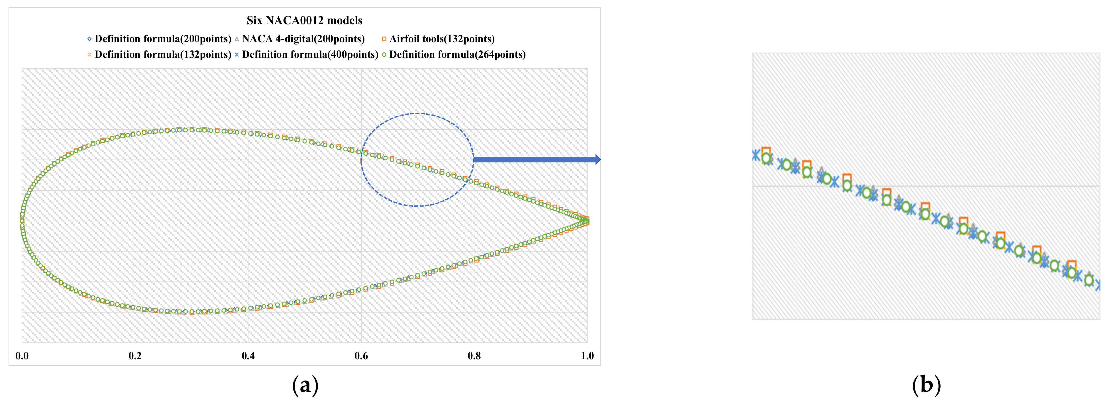
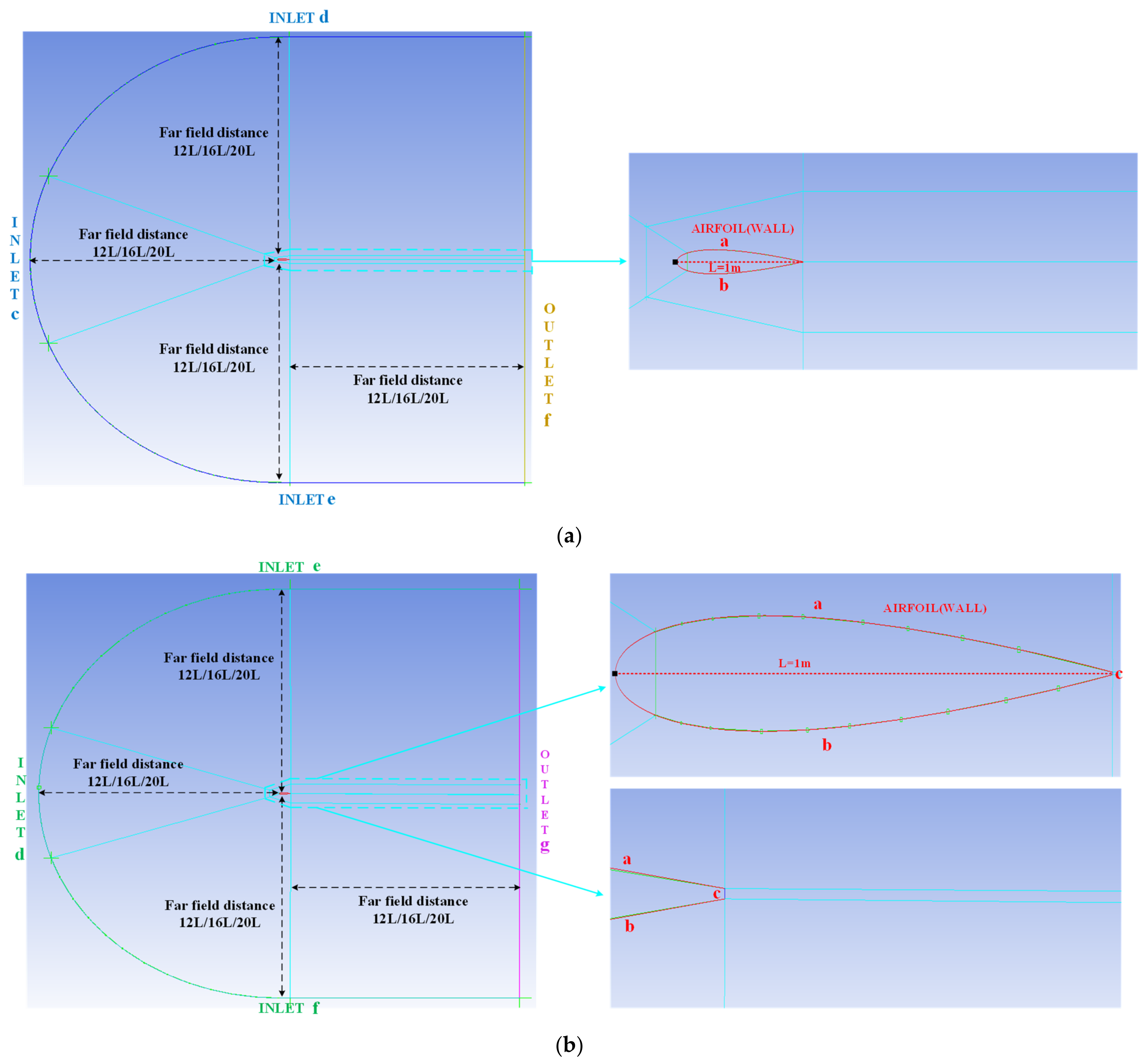
2.1.1. NACA0012 Models and External Flow Field of the Computational Domain

The following are three general ways to establish the NACA0012 airfoil model:
  • Airfoil tools, which refers to the UIUC Airfoil coordinates database and provides 132 data points. It should be noted that the ends of the established NACA0012 trailing edge based on Airfoil tools are not closed, and we need to connect the ends manually to form the blunt trailing edge. If the ends of the trailing edge are not connected, after being imported into meshing tools, a blunt elliptic shape will be formed at the trailing edge of the generated two-dimensional airfoil, failing mesh generation
  • NACA 4-digit airfoil generator, which provides a maximum of 200 data points. It gives a close trailing edge option to form the sharp trailing edge.
  • The definition formula, which is Equation (1), where x is the x-axis location and y is the y-axis location.
y = ± 0.594689181 × [ 0.298222773 × x 1 / 2 0.127125232 × x 0.357907906 × x 2 + 0.291984971 × x 3 0.105174606 × x 4 ]
Considering there are two sources of data points, to further analyze the influences of different data points source and data points’ numbers on the simulation accuracy, six NACA0012 models are built, which include one blunt trailing edge shape model and five sharp trailing edge shape models. For the blunt trailing edge shape model, we apply the Airfoil tools to establish. For the five sharp trailing edge models:
  • The NACA4-digital generator.
  • The definition formula applies 132 data points provided by Airfoil tools.
  • The definition formula applies 200 data points provided by the NACA4 generator.
  • The definition formula applies 264 data points. We double the 132 points provided by Airfoil tools to 264 points by adding the average value between two points.
  • The definition formula applies 400 data points by doubling 200 points from NACA4.
Figure 1a depicts the above six NACA0012 models and there are apparent location differences among models, as shown in Figure 1b. The Airfoil tools and the NACA 4-digit airfoil generator directly provide the data points for modeling, which do not give the related formulas. We then adopt curve fitting to produce the related formulas based on the existing data points. For the Airfoil tools, the fitting formula is
y = ± a 1 x 8 + a 2 x 7 + a 3 x 6 + a 4 x 5 + a 5 x 4 + a 6 x 3 + a 7 x 2 + a 8 x + a 9
where a 1 = −32.25, a 2 = 139.4, a 3 = −249.5, a 4 = 239, a 5 = −132.5, a 6 = 43.15, a 7 = −8.247, a 8 = 0.9256, a 9 = 0.005819 and R 2 = 0.9971.
For the NACA 4-digit airfoil generator, the fitting formula is
y = ± a 1 x 8 + a 2 x 7 + a 3 x 6 + a 4 x 5 + a 5 x 4 + a 6 x 3 + a 7 x 2 + a 8 x + a 9
where a 1 = −31.18, a 2 = 134.8, a 3 = −241.4, a 4 = 231.4, a 5 = −128.5, a 6 = 41.93, a 7 = −8.052, a 8 = 0.9116, a 9 = 0.006113 and R 2 = 0.9975. Therefore, the differences among different NACA0012 models shown in Figure 1 could be represented through the subtraction between the related formulas.

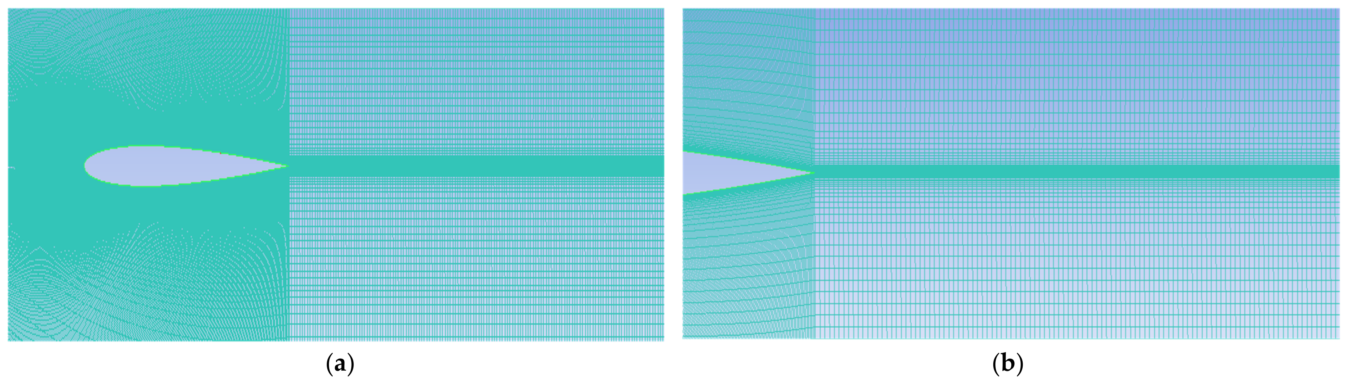
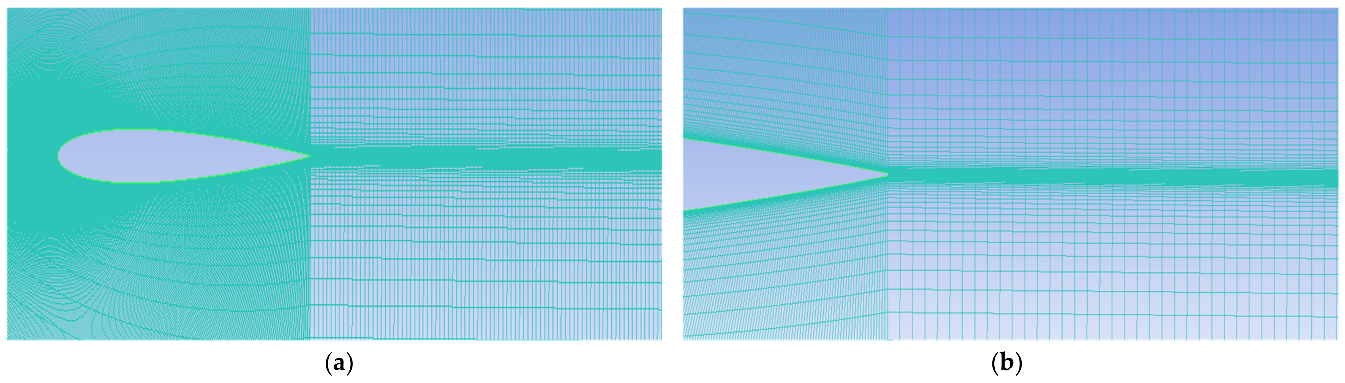
2.1.2. Gird Division

Considering that the ICEM CFD and fluent of ANSYS are adopted to perform numerical simulations, we consult the official reference materials and ANSYS suggests that a more realistic far-field distance for external flow field simulation of the computational domain should be 12–20 times the chord length (L) of the airfoil [22]. Moreover, the calculation resources are limited and a larger far-field distance would result in a larger mesh number, and the maximum number of it in grid independency tests would easily exceed 1,200,000, which is beyond the capacity of the computer and the numerical calculations are difficult. Therefore, in this paper, considering the official suggestion and the limited calculation resources, we establish the computational domain within 20 chords. L is 1 m and 12L/16L/20L are chosen to establish the C-type mesh topology to minimize the skewness of a near-wall mesh. Figure 2a demonstrates the computational domain for the sharp trailing edge, where the square black dot represents the origin of the coordinate system. The block at the trailing edge is folded, which is highlighted in cyan. Considering that the meshing adjacent to the airfoil surface has a significant impact on the CFD simulation, the block close to the airfoil surface is divided. The “INLET” is the input boundary, which comprises lines c, d, and e. The “OUTLET” is the output boundary, which comprises line f. The “AIRFOIL” is the wall boundary, which comprises lines a and b. The computational domain for the blunt trailing edge is shown in Figure 2b; similarly, the grid refinements region is highlighted in cyan, and unlike the sharp trailing edge, the block at the trailing edge is retained, which is like a “fishtail”. The “INLET” is the input boundary, which comprises lines d, e, and f. The “OUTLET” is the output boundary, which comprises line g. The “AIRFOIL” is the wall boundary, which comprises lines a, b, and c.

2.1.3. Mesh Parameters

The airfoil surface is the main mean vorticity and turbulence source, where the momentum and scalar transports change vigorously, and the numerical variables have high gradients. Hence, the meshing of the near wall region has a key influence on the simulation fidelity. Near the airfoil surface, there exists a thin layer called the boundary layer, which contains all the viscous effects. A successful wall-bounded turbulent flow prediction is closely related to the viscous boundary layer representation, and firstly, we should ensure the first layer cells of the boundary layer ( y H ) are in the viscous sublayer. Generally speaking, for high accuracy demands on the wall boundary layer simulations, the y + of the near wall meshes with 1 is recommended [23]. The y + is calculated by the following Equation:
y + = ρ y P u τ μ
where ρ is the flow density, y P is the height from the centroid of the wall adjacent cells to the wall, u τ is the friction velocity, μ is the flow dynamic viscosity and y H could be obtained by doubling y P . For the Tt is 81.2 K, ρ is about 0.0247 kg/m3. Then according to Equation (5), the speed of propagation of acoustic disturbances in the air (speed of sound Cair) is 180.6 m/s. The Mach number is 10 and Ut is 1806 m/s, therefore, according to Equation (6), μ is about 4.46082 × 10⁻⁵ paⅹs.
C a i r = 20.05 T
R e = ρ U L μ
And now we just have to calculate u τ to confirm y H . As the Re is less than 1 × 10⁹, the below empirical correlation formulation to estimate the skin friction coefficient ( C f ) is used [24]:
C f = [ 2 log 10 ( R e ) 0.65 ] 2.3
After C f is calculated, we could obtain the wall shear stress ( τ W ):
τ W = 1 2 ρ U 2 C f
Now, u τ is achieved by:
u τ = ( τ W ρ ) 0.5
Finally, y H is calculated:
y H = 2 y P
It is worth noting that C f is an empirical formulation, so the computed y H value is an estimate and would need to be updated using information from the CFD analysis. Initially, y + is 1 and y H is 4.65 × 10⁻⁵ m according to Equation (4) to Equation (10), while during the simulation process, the test results show that the maximum y + value exceeds 1. We further lower the y + value and the tests show that the value of 0.08 could guarantee the maximum y + of airfoil surface within 1 and the corresponding y H is 3.5 × 10⁻⁶ m. The close views of meshes near the WALL region and different trailing edge shapes are as shown in Figure 3 and Figure 4. The mesh used in the present computations does not have such (desirable) mesh clustering around the shock or the alignment with it. This fact should be borne in mind while comparing the sharpness of the shock.
Secondly, we need to perform different mesh levels to ensure grid independency, and in every refinement, the number of total grids is 1.4 times more. We take the sharp trailing edge (based on NACA4) adopting the SST k-omega as an example and the other cases present similar errors as we exemplified the errors of the meshes for the sharp trailing edge. Under x/L locations from −0.007 m to 0 m, the ratios between P and Pt and T and Tt, and the error ratios compared to the reference data are shown in Table 1, Table 2 and Table 3. At 12 m far-field distance, the mean error ratios and the total mean error ratio of (P/Pt, T/Tt) of three level meshes are (10.2%, 6.98%, 8.59%), (2.28%, 3.96%, 3.12%), and (9.88%, 4.21%, 7.05%). Similarly, the values at a far-field distance of 16 m are (9.96%, 6.03%, 8.35%), (6.23%, 3.25%, 4.74%), and (9.36%, 4.36%, 6.86%), and those of 20 m far-field distance are (6.78%, 6.84%, 7.97%), (3.15%, 4.14%, 3.65%), and (5.64%, 5.38%, 5.51%). Compared with the total mean error ratios of 588,000, the calculation accuracies of 418,000 and 828,000 of 12 m far-field distance are dropping and the decline degrees are −175% and −126%. Similarly, the calculation accuracies of 418,000 and 828,000 of far-field distances of 16 m and 20 m are also dropped and the decline degrees are −76%, −45%, −118%, and −51%. Under x/L locations from 0 m to 0.7 m, the pressure coefficient Cp, entropy, and the error ratios compared to the reference data are shown in Table 4, Table 5 and Table 6. At 12 m far-field distance, the mean error ratios of (Cp, entropy) of three-level meshes are (12.41%, 4.79%), (8.31%, 3.85%), and (11.2%, 4.4%). Similarly, the values at a far-field distances of 16 m are (11.9%, 4.2%), (5.5%, 3.14%), and (8.79%, 4.06%), and those of 20 m far-field distance are (12.29%, 4.86%), (8.86%, 4.15%), and (11.51%, 4.51%). Hence, the performances of the 588,000 are preferred. Meanwhile, considering the limited computing resources, the mesh with 588,000 is adopted.
Thirdly, the mesh evaluation quality metrics, the aspect ratio, and the determinant need to be checked to ensure the mesh is sufficient. Attention should be paid to the aspect ratio, for the values of y + and y H are very small, the maximum aspect ratio value could exceed 10,000 easily, which means the floating-point overflow or the calculation divergence may occur and the simulation would fail. In this paper, we confirm, through CFD tests, the proper aspect ratio and the determinant values. For the sharp trailing edge, the maximum aspect ratio and the minimum determinant are (2110, 0.84), (3310, 0.881), and (4460, 0.873) at far-field distances of 12 m, 16 m, and 20 m, respectively. For the blunt trailing edge, the maximum aspect ratio and the minimum determinant are (2760, 0.894), (3680, 0.886), and (4770, 0.827) at far-field distances of 12 m, 16 m, and 20 m, respectively.

2.2. Numerical Methods

2.2.1. Turbulence Models

At middle to high Re, the unsteady random motion could be observed, which is called turbulence. By the NS equations, turbulence could be described mathematically. For the enormous demand for the computational resources of the direct numerical simulation (DNS) in practice, the Reynolds average (RANS) method is widely used [25]. RANS introduces additional unknown terms into equations, which need to be provided by suitable turbulence models. Therefore, the adopted turbulence model would determine the simulation quality. Typical RANS models include k-epsilon and k-omega, and SA. k-epsilon are two-equation models, which are designed for traditional industrial CFD and have disadvantages of insensitivity to the boundary layer separation and adverse pressure gradients [26]. For the external aerodynamics studied in this paper, the k-epsilon is not suitable. The standard k-omega models, however, are better at predicting adverse pressure gradient boundary layer flows and have advantages relative to the k-epsilon. Further, SST k-omega overcomes the deficiency of standard k-omega models in that the solution of which has a strong sensitivity to the freestream values. So, the SST k-omega turbulence model is suitable for external aerodynamic flows [27]. It should be noted that excessive turbulence energy generation is a draw-back of the SST k-omega and the production limiter is suggested. The SA model is specifically designed for aeronautics and aerospace applications involving wall-bounded flows [28]. Therefore, the SST k-omega and SA turbulence models are selected.
SST k-omega is a two-equation turbulence model and the turbulent viscosity μ t is computed as a function of the turbulence kinetic energy k and the specific dissipation rate ω . K and ω are obtained from the following transport equations:
t ρ k + x i ρ k u i = x j Γ k k x j + G k Y k + S k + G b
t ( ρ ω ) + x i ( ρ ω u i ) = x j ( Γ ω ω x j ) + G ω Y ω + S ω + G ω b + D ω
SA is a one-equation RANS turbulence model and the transport equation for the turbulent kinematic viscosity v ˜ is:
t ρ v ˜ + x i ρ v ˜ u i = 1 σ v ˜ x j μ + ρ v ˜ v ˜ x j + C b 2 ρ v ˜ x j 2 + G v Y v + S v ˜
Attention should be paid to the modified turbulent viscosity order selection of the SA turbulence model. Taking the sharp trailing edge (based on NACA4), adopting SA at three far-field distances as examples and the comparison of the results between two order types are shown in Table 7. Unlike under the incompressible environment [3], the mean error ratios of P/Pt and T/Tt of the first-order under 12 m far-field distance are (9.18%, 4.96%), and those of the second-order are (4.42%, 2.16%). Similarly, the results under 16 m and 20 m far-fields distances are (9.38%, 7.71%), (5.33%, 5.24%), (7.42%, 7.12%), and (4.69%, 4.28%) in turn and the error ratios of the second-order are preferred, hence, the second-order upwind Modified turbulent viscosity is chosen.

2.2.2. Flux Type

At the hypersonic speed, we adopt the density-based solver employing time-derivative preconditioning [29]. The system governing equations in vector form is as follows:
Γ t V Q d V + F G × d A = V H d V
where V and A represent an arbitrary control volume and surface area, the source terms like energy sources and body forces are contained in vectors H, the vectors Γ , F, and G are defined as follows and the parameter Θ is [29]:
Γ = Θ 0 0 0 ρ T Θ u ρ 0 0 ρ T u Θ v 0 ρ 0 ρ T v Θ w 0 0 ρ ρ T w Θ H δ ρ u ρ v ρ w ρ T H + ρ C p ,   F = ρ v ρ v u + p i ^ ρ v v + p j ^ ρ v w + p k ^ ρ v E + p v ,   G = 0 τ x i τ y i τ z i τ i j v j + q   Θ = 1 U r 2 ρ T ρ C p
Generally speaking, the flux vector F could be evaluated in two common ways:
  • ROE flux-difference splitting scheme [30]. At each face, the discrete flux is expressed as:
F = 1 2 F R + F L 1 2 Γ A ^ δ Q
  • AUSM flux-vector splitting scheme [31], which provides a numerical flux form to avoid using explicit artificial dissipation.
F = m f φ + p i
Ref. [32] investigates the calculation accuracy of ROE and AUSM. Taking the flow around the cylinders as an example, the results demonstrate that the numerical results of those two flux types are close to the reference data, based on which we have performed the influence analysis of simulation parameters on prediction accuracy under hypersonic speed based on the wedge section [21]. The conclusions tell that the AUSM flux type performs better than those of the ROE. Similarly, in this paper, according to Refs. [21,32], these two flux types are also adopted. We take the NACA0012 airfoils as examples to perform simulations to investigate the related calculation accuracy influence under hypersonic speed.

2.3. Numerical Simulations

At hypersonic speeds, the air density adopts ideal gas for the reasons below: (1) According to Ref [33], we adopt the pressure far field boundary condition to model a free stream condition at infinity for the aerodynamic application, and this boundary type is available only for compressible flows. For compressible flows, the ideal gas is the appropriate density relationship. In the ANSYS fluent, the pressure far field boundary condition is applicable only when the density is calculated using the ideal gas. Using it for other flows is not permitted. (2) The ideal gas has the limitation that it is approximately valid for the low-pressure gas region of the PT and PV diagrams. The ideal gas behavior can be expected when P/Pc ≪ 1, where Pc is the critical pressure of air flow and the value is 3.77 MPa. If the flow conditions correspond to the case, the ideal gas could be adopted in the simulation. Otherwise, it could not be used. In this paper, the initial pressure value of free stream is 576 pa and the maximum pressure value is about 73728 pa. The maximum value of P/Pc is about 0.019, which corresponds to the above case. The viscosity adopted the three-coefficient Sutherland Law, and the specific heat at constant air pressure is 1006.43 j/kg-k. One should note that in this paper, for the SST k-omega turbulence model, the turbulence specification method of the input boundary adopts the intensity and viscosity ratio, the values of which are 1% and 1. The effective diffusivities Γ k = μ + μ t σ k ,   Γ ω = μ + μ t σ ω . The turbulent viscosity μ t = ρ k ω 1 max 1 α * , S F 2 a 1 ω , where α * = α * α 0 * + R e t / R k 1 + R e t / R k , R e t = ρ k μ ω ,   α 0 * = β i / 3 , F 2 = tanh ϕ 2 2 and   ϕ 2 = max 2 k 0.09 ω y , 500 μ ρ y 2 ω . The applied model constants are as follows: σ k , 1 = 1.176 , σ ω , 1 = 2.0 , σ k , 2 = 1.168 , α 1 = 0.31 , β i , 1 = 0.075 , β i , 2 = 0.0828 , and other model constants have the same values as for the standard k-omega model [34]: α * = 1 ,   α = 0.52 ,   α 0 = 1 9 ,   β * = 0.09 ,   R β = 8 ,   R k = 6 ,   R ω = 2.95 ,   ξ * = 1.5 ,   M t 0 = 0.25 . For the SA turbulence model, the input boundary adopts the turbulent viscosity ratio and the value is 1. the turbulent viscosity μ t = ρ v ˜ f v 1 , where the viscous damping function f v 1 = χ 3 χ 3 + C v 1 3 and χ v ˜ v . The production term G v = C b 1 ρ S ˜ v ˜ , where S ˜ S + v ˜ κ 2 d 2 f v 2 and f v 2 = 1 χ 1 + χ f v 1 . The destruction term Y v = C ω 1 ρ f ω v ˜ d 2 , where f ω = g 1 + C ω 3 6 g 6 + C ω 3 6 1 / 6 , g = r + C ω 2 r 6 r and r v ˜ S ˜ κ 2 d 2 . The applied model constants are as follows, which have the default values [28]. C b 1 = 0.1355 ,   C b 2 = 0.622 ,   σ v ˜ = 2 3 ,   C v 1 = 7.1 ,   C ω 2 = 0.3 ,   C ω 3 = 2.0 , κ = 0.4187 , C ω 1 = C b 1 κ 2 + 1 + C b 2 σ v ˜ . For the convection terms of each flow governing equation, we should confirm the appropriate discretization scheme. The discrete values of scalar φ are stored at the cell centers and face values φ f are required, which are interpolated from cell center values by the upwind scheme. In a general way, we use the second-order upwind discretization. Gradients are used for constructing scalar values at the cell faces, calculating secondary diffusion terms and velocity derivatives, and there are cell-based, node-based, and least-squares cell-based three common schemes available. The least-squares cell-based averaging scheme has the advantage of being as accurate as the node-based scheme and having fewer demands for computing resources than the node-based scheme. So, we adopt the least-squares cell-based scheme for gradient reconstruction. To avoid spurious oscillations appearing near shocks or near rapid local changes in flows, the TVD slope limiter is selected as the gradient limiter [35], which uses the Minmod function to limit and clip the reconstructed solution overshoots and undershoots on the cell faces.
Table 8 demonstrates the key parameters adopted in the CFD simulations. Taking the six NACA0012 models, combined with three far-field distances, SST turbulence model, and ROE flux type as examples, the numerical results and error ratios are provided in Table 9, Table 10 and Table 11.

3. Results and Discussion

According to the results obtained from CFD simulations in Section 2, we perform a detailed influence analysis on the numerical simulation accuracy from the following four aspects: the NACA0012 models, the far-field distances, the turbulence models, and the flux types.

3.1. NACA0012 Models

Based on 12 m/16 m/20 m far-field distances, the SST k-omega and SA turbulence models, and ROE and AUSM flux types, we can make the following simulation configurations: SST + 12 m (ROE/AUSM), SA + 12 m (ROE/AUSM), SST + 16 m (ROE/AUSM), SA + 16 m (ROE/AUSM), SST + 20 m (ROE/AUSM) and SA + 20 m (ROE/AUSM). Therefore, for each NACA0012 model described in Section 2.1.1, applying the parameters in Table 8, twelve groups of simulations is performed. The numerical results of P/Pt, T/Tt, and U/Ut and the corresponding reference data are illustrated in Figure 5, Figure 6, Figure 8, Figure 9, Figure 11, Figure 12, Figure 14, Figure 15, Figure 17, Figure 18, Figure 20 and Figure 21. We then calculate the related mean error ratios of P/Pt, T/Tt, and U/Ut and the results are provided in Table 12, Table 13, Table 14, Table 15, Table 16 and Table 17. The optimal results and the related accuracy improvements under different configurations for each NACA0012 model are obtained, which are shown in Figures 7, 10, 13, 16, 19 and 22.

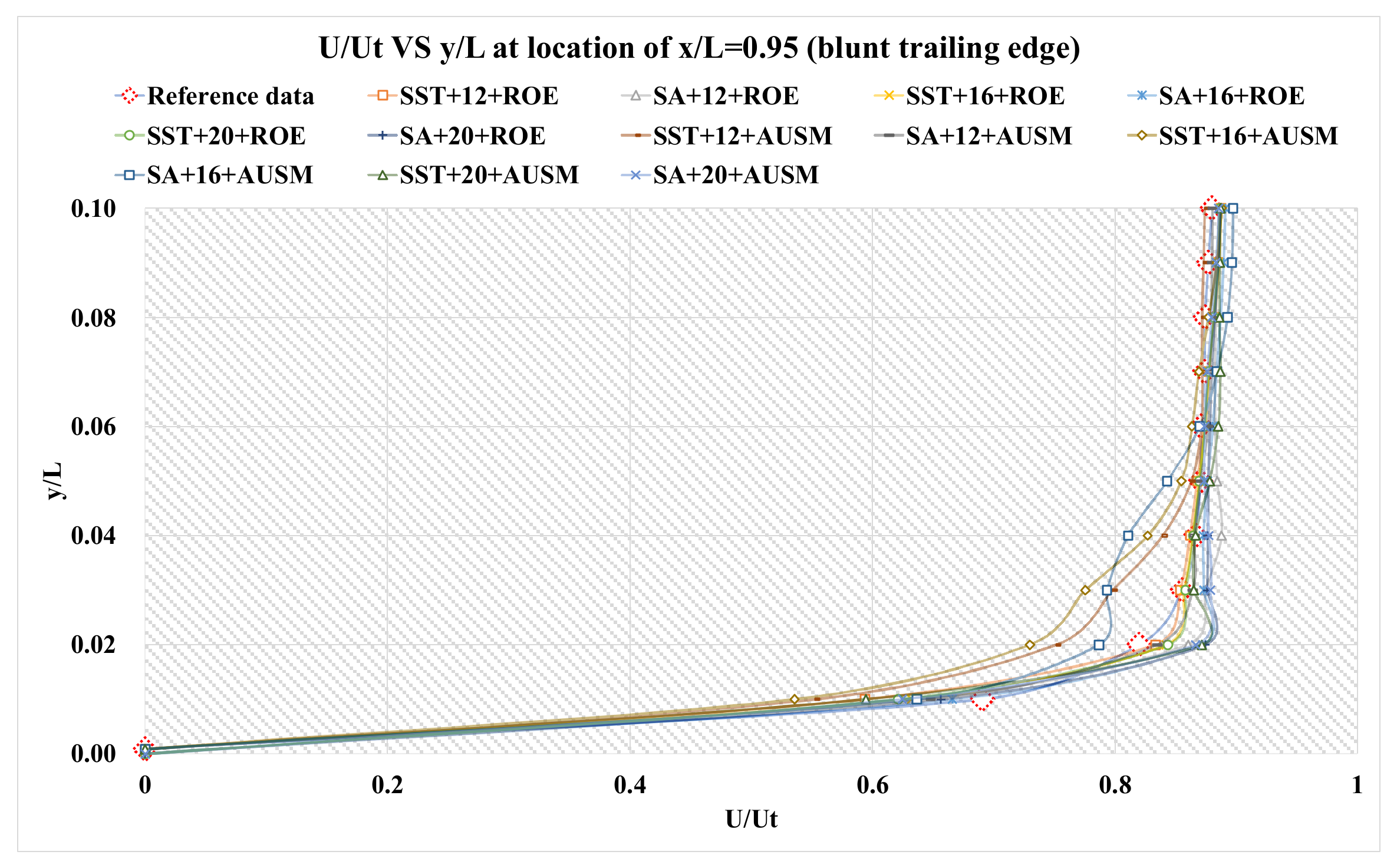
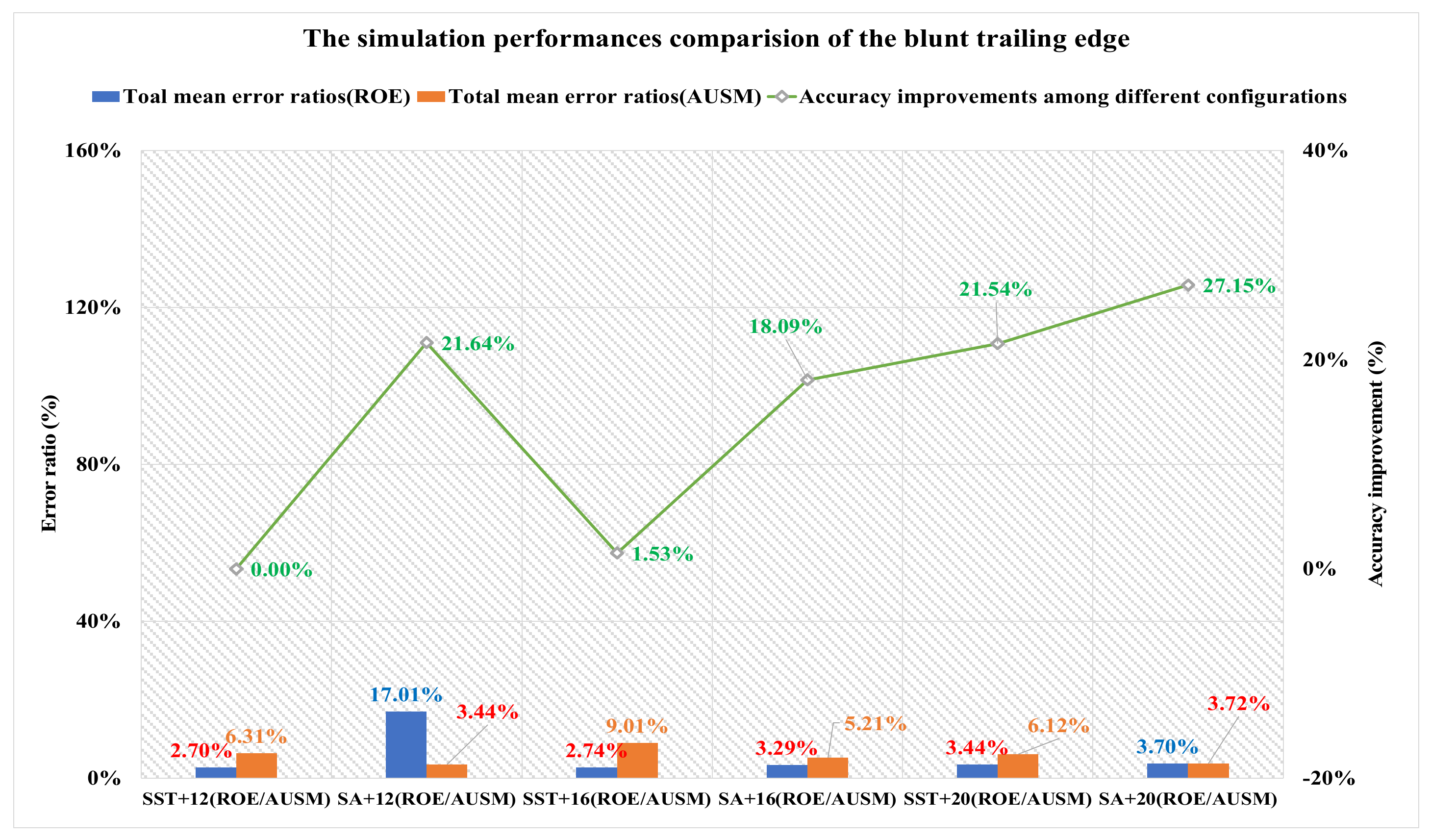
3.1.1. Results of the Blunt Trailing Edge

Figure 5 shows the distributions of P/Pt and T/Tt of reference data and simulation data, where the x-axis is the x/L location and the y-axis is the result. Figure 6 provides the distributions of U/Ut at location of x/L = 0.95, where the x-axis is the result and the y-axis is the y/L location. The corresponding mean error ratios are shown in Table 12 and we could confirm the optimal results under different configurations, as shown in Figure 7, which are highlighted in red. As to the far-field distance, the minimums of three distances are 2.70%, 2.74%, and 3.44%. As to the turbulence model, the best result of SST is 2.70% and that of SA is 3.29%. As to the flux type, the best performance of ROE is 2.70% and that of AUSM is 3.44%. In conclusion, the minimum total mean error ratio is 3.25%, which is achieved by SST + 12 m (ROE). Compared with optimal results of other simulation configurations, the corresponding accuracy gains are 21.64%, 1.53%, 18.09%, 21.54%, and 27.15% respectively.
Table 12. The mean error ratios of P/Pt, T/Tt, and U/Ut of the blunt trailing edge.
Simulation
Configurations
Mean Error Ratios under Different Configurations
ROEAUSM
P/PtT/TtU/UtP/PtT/TtU/Ut
SST + 12 m1.97%4.52%1.60%8.94%5.91%4.07%
SA + 12 m24.04%24.61%2.39%3.62%5.56%1.14%
SST + 16 m2.20%4.49%2.74%8.16%13.63%5.25%
SA + 16 m3.52%4.38%3.29%5.89%6.11%3.63%
SST + 20 m5.27%3.36%3.44%9.47%6.02%2.86%
SA + 20 m6.40%2.70%3.70%7.27%1.68%2.22%

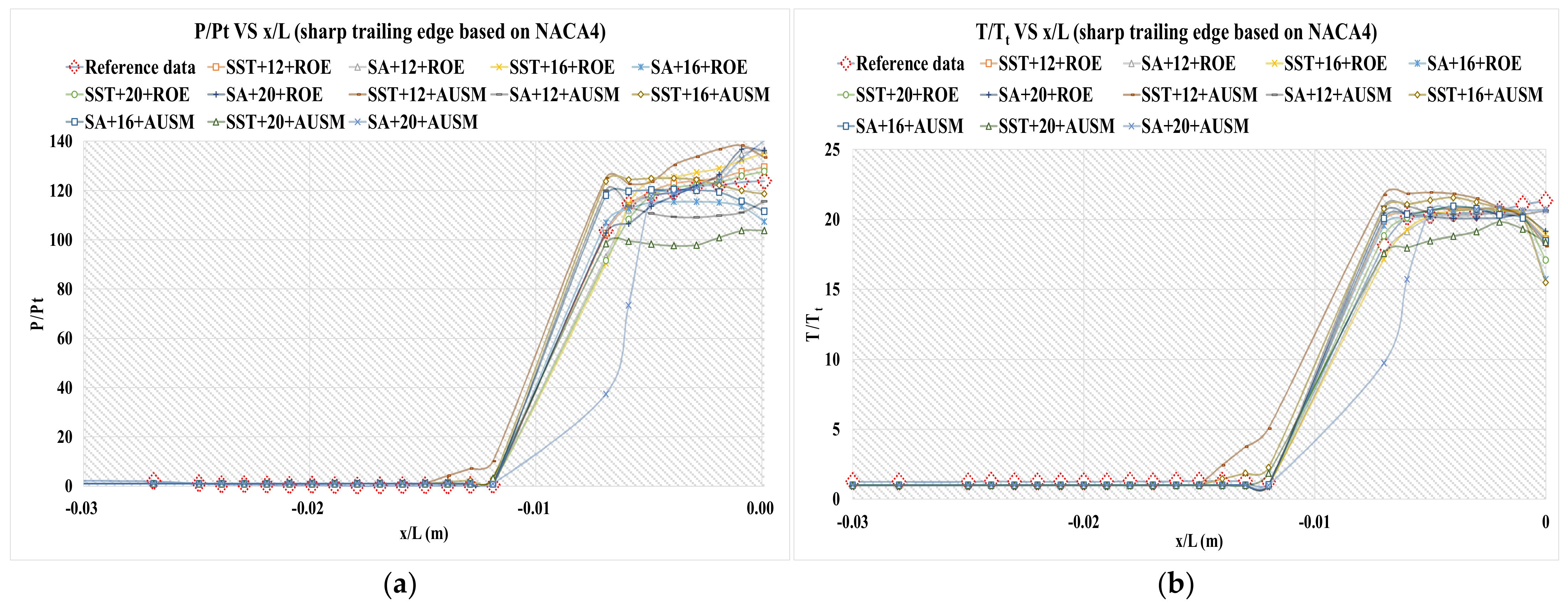
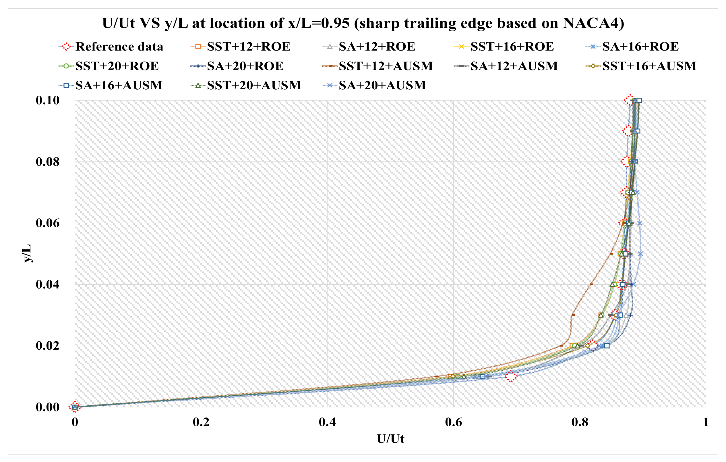
3.1.2. Results of the Sharp Trailing Edge Based on NACA4-Digital Generator

Figure 8 and Figure 9 illustrate the distributions of P/Pt, T/Tt, and U/Ut of numerical data and reference data and Table 13 provides the corresponding mean error ratios. Figure 10 provides the optimal performances under different configurations and those are highlighted in red. For the far-field distance, the finest results for the three distances are 2.42%, 3.80%, and 3.19%. For the turbulence model, the minimum result of SST is 2.42%, and that of SA is 2.83%. For the flux type, ROE has a minimum mean error ratio of 2.42%, and that of AUSM is 3.80%. In general, the SST + 12 m, combined with ROE has the best performance of 3.12%. Compared with optimal results of other simulation configurations, the corresponding accuracy advances are 14.29%, 38.54%, 36.17%, 24.01%, and 32.02%, respectively.
Table 13. The mean error ratios of P/Pt, T/Tt, and U/Ut of the sharp trailing edge based on NACA4.
Simulation
Configurations
Mean Error Ratios under Different Configurations
ROEAUSM
P/PtT/TtU/UtP/PtT/TtU/Ut
SST + 12 m2.28%3.96%1.04%10.41%8.54%4.38%
SA + 12 m4.42%2.16%1.90%8.52%3.55%1.40%
SST + 16 m6.23%3.25%2.36%5.96%8.19%2.07%
SA + 16 m5.33%5.24%1.61%5.12%4.57%1.71%
SST + 20 m3.15%4.14%2.28%15.30%8.00%2.38%
SA + 20 m4.69%4.28%1.73%15.45%9.74%2.06%

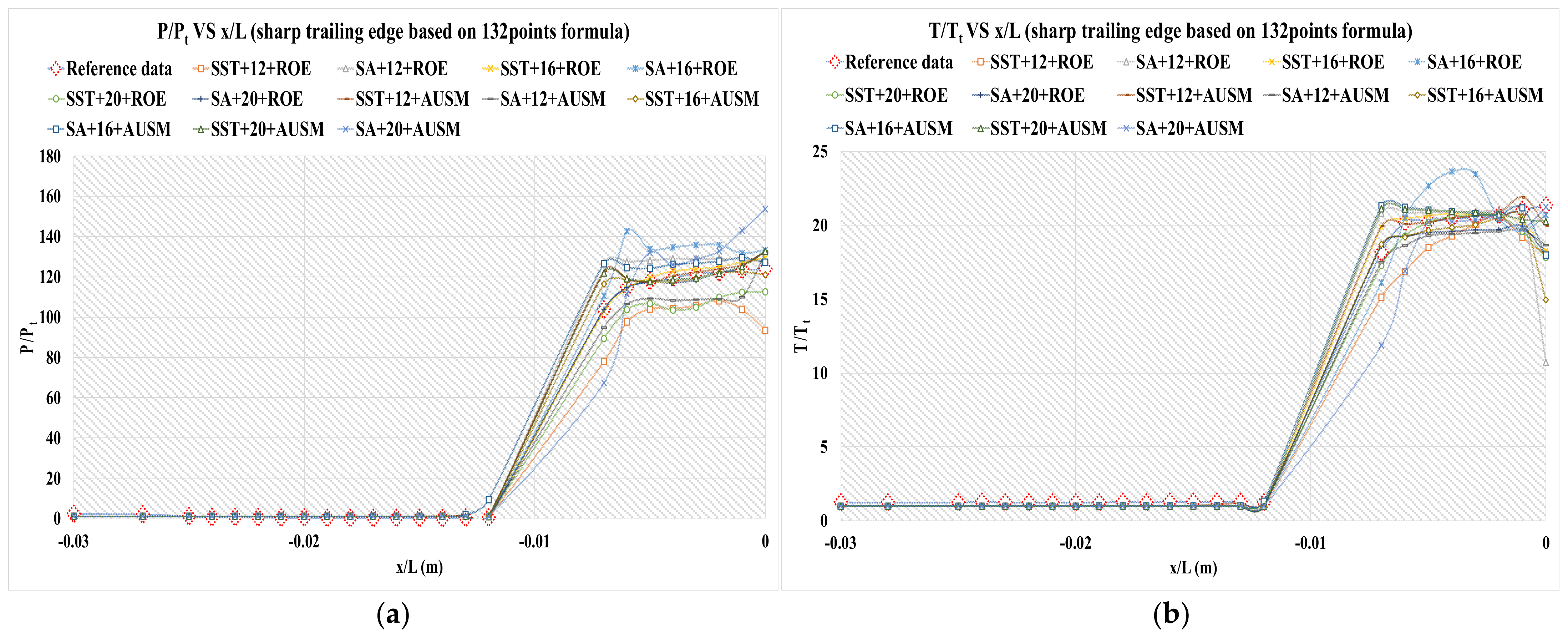
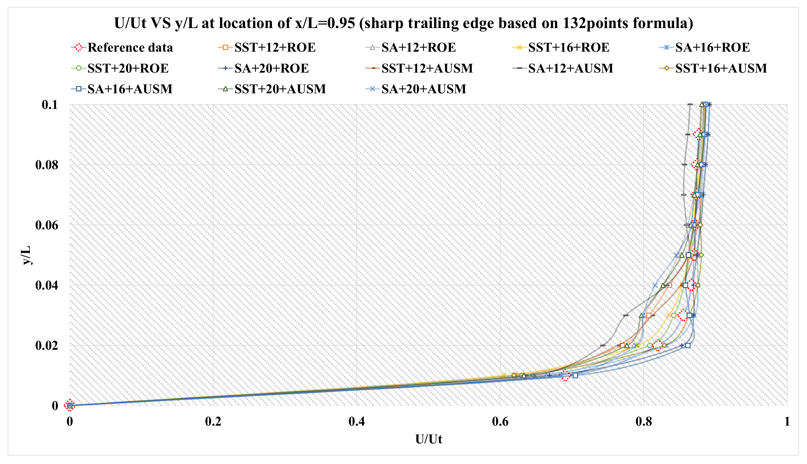
3.1.3. Results of the Sharp Trailing Edge Based on Definition Formula Applying 132 Points

Figure 11 and Figure 12 illustrate the distributions of P/Pt, T/Tt, and U/Ut of numerical data and reference data and the corresponding mean error ratios under different locations are calculated and shown in Table 14. The optimal total mean error ratios under different configurations are displayed in Figure 13, which are highlighted in red. In terms of the far-field distance, the preferred results for the three distances are 3.14%, 2.64%, and 2.98%. In terms of the turbulence model, the minimum result of SST is 2.64%, and that of SA is 2.98%. In terms of the flux type, ROE has a finest mean error ratio of 2.64%, and that of AUSM is 3.14%. Comparing total mean error ratios for all configurations, the SST + 16 m, adopting ROE behaves the best, and the related accuracy improvements are 15.82%, 58.62%, 45.07%, 31.82%, and 11.29%, respectively.
Table 14. The mean error ratios of P/Pt, T/Tt, and U/Ut of the sharp trailing edge based on 132 points.
Simulation
Configurations
Mean Error Ratios under Different Configurations
ROEAUSM
P/PtT/TtU/UtP/PtT/TtU/Ut
SST + 12 m16.13%9.27%2.95%4.32%2.88%2.21%
SA + 12 m8.58%9.70%2.41%8.91%6.31%3.91%
SST + 16 m2.14%4.21%1.57%2.78%6.14%1.78%
SA + 16 m11.85%8.20%1.66%7.32%5.83%1.26%
SST + 20 m11.00%4.36%1.61%4.14%4.64%2.83%
SA + 20 m1.76%5.58%1.59%13.73%7.50%2.34%

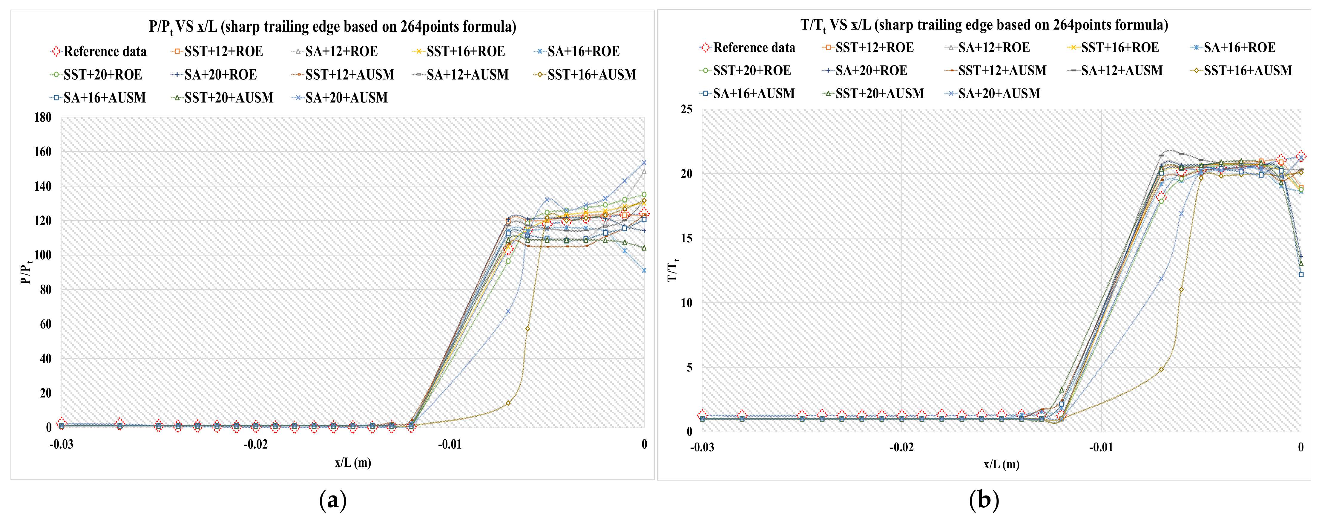
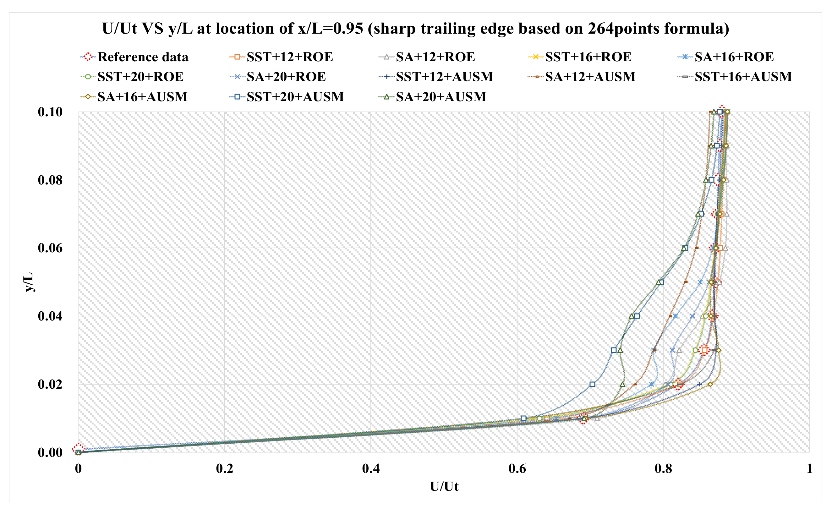
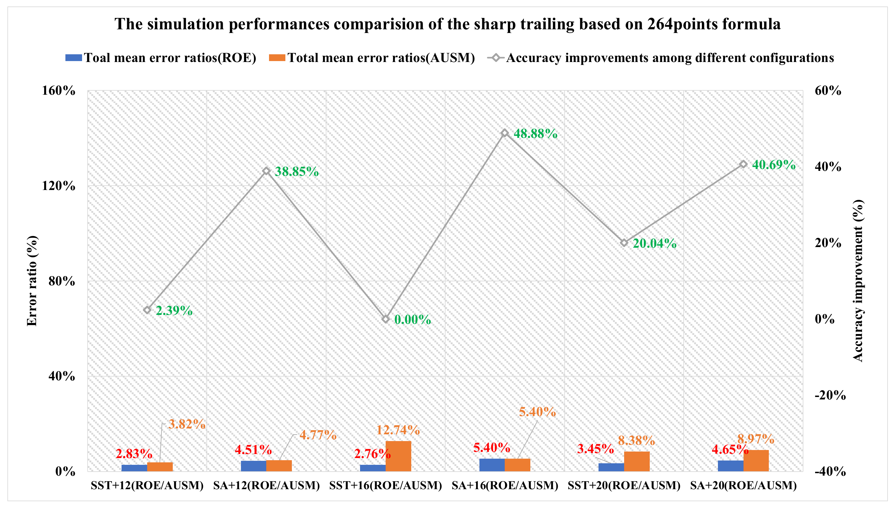
3.1.4. Results of the Sharp Trailing Edge Based on Definition Formula Applying 264 Points

The distributions of P/Pt, T/Tt, and U/Ut of simulation data and reference data are presented in Figure 14 and Figure 15, and Table 15 shows the corresponding mean error ratios. Figure 16 gives the optimal total mean error ratios under different configurations, and those are highlighted in red. For the far-field distance, the finest results for the three distances are 2.83%, 2.76%, and 3.45%. For the turbulence model, the minimum result of SST is 2.76%, and that of SA is 4.51%. For the flux type, ROE has a minimum value of 2.76%, and that of AUSM is 3.82%. In general, the SST + 16 m, combined with ROE has the best performance of 2.76%. Compared with optimal results of other simulation configurations, the corresponding accuracy developments are 2.39%, 38.85%, 48.88%, 20.04%, and 40.69%, respectively.
Table 15. The mean error ratios of P/Pt, T/Tt, and U/Ut of the sharp trailing edge based on 264 points.
Simulation
Configurations
Mean Error Ratios under Different Configurations
ROEAUSM
P/PtT/TtU/UtP/PtT/TtU/Ut
SST + 12 m3.44%3.81%1.23%7.95%2.81%0.70%
SA + 12 m8.42%3.39%1.73%5.19%5.03%4.08%
SST + 16 m2.62%4.00%1.65%18.77%17.84%1.62%
SA + 16 m8.82%4.45%2.92%6.81%8.17%1.23%
SST + 20 m6.03%2.75%1.56%9.67%8.47%6.99%
SA + 20 m5.11%7.58%1.26%13.73%7.50%5.67%

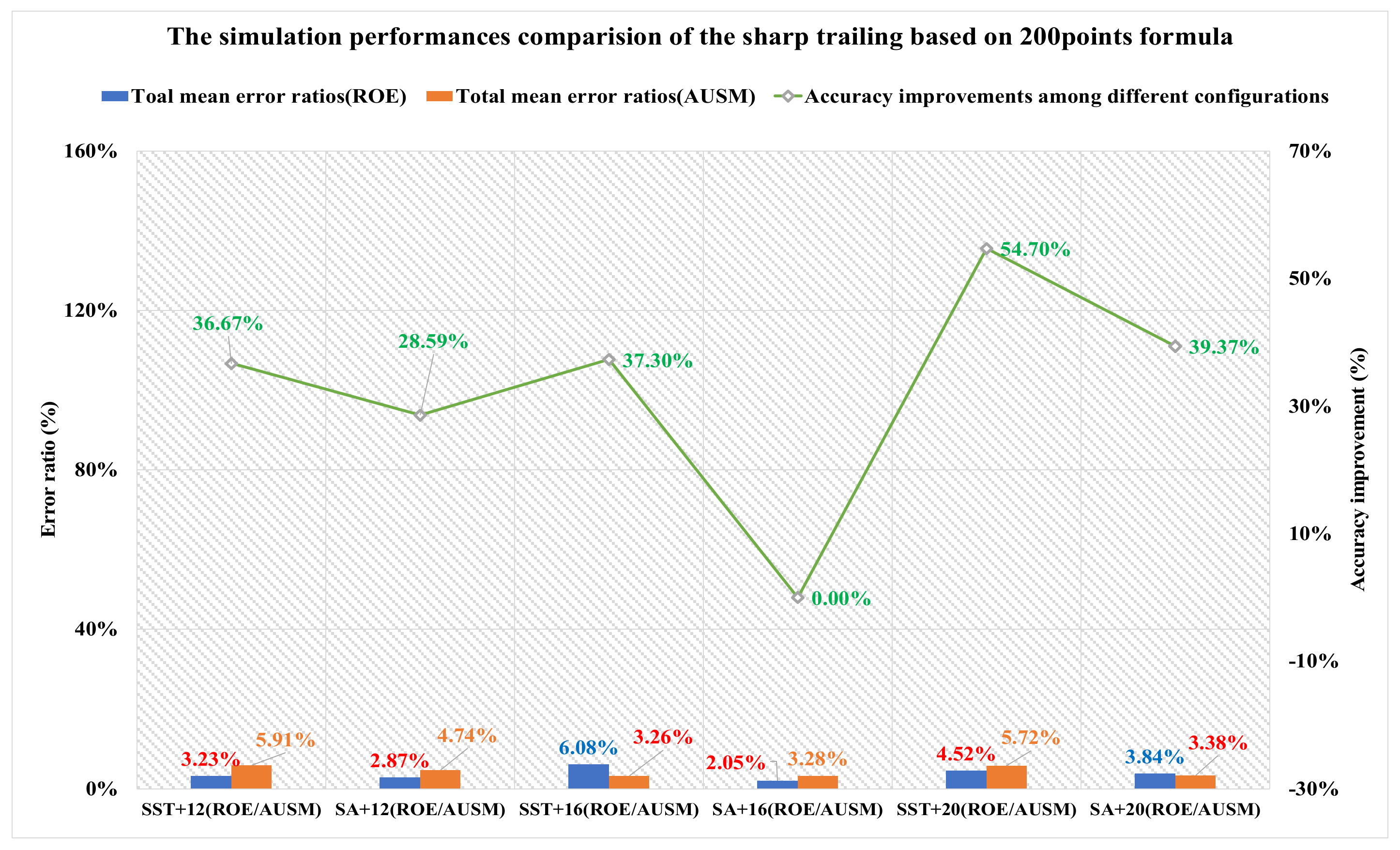
3.1.5. Results of the Sharp Trailing Edge Based on Definition Formula Applying 200 Points

The distributions of P/Pt, T/Tt, and U/Ut of simulation data and reference data are presented in Figure 17 and Figure 18, and Table 16 shows the corresponding mean error ratios. We then calculate the total mean error ratios and the optimal performances of different configurations are highlighted in red in Figure 19. As to the far-field distance, the minimums of three distances are 2.87%, 2.05%, and 3.38%. As to the turbulence model, the best result of SST is 3.23%, and that of SA is 2.05%. As to the flux type, ROE has the best performance of 2.05%, and that of AUSM is 3.26%. Based on the comparison among optimal total mean error ratios under different configurations, we could conclude that the SA + 16 m combined with ROE behaves the best. The optimal total mean error ratio is 2.05%, and the relative accuracy increases are 36.67%, 28.59%, 37.30%, 54.70%, and 39.37%.
Table 16. The mean error ratios of P/Pt, T/Tt, and U/Ut of the sharp trailing edge based on 200 points.
Simulation
Configurations
Mean Error Ratios under Different Configurations
ROEAUSM
P/PtT/TtU/UtP/PtT/TtU/Ut
SST + 12 m4.86%3.88%0.96%8.02%7.94%1.77%
SA + 12 m5.87%1.18%1.55%7.83%4.63%1.76%
SST + 16 m8.58%7.83%1.83%3.74%4.06%2.00%
SA + 16 m2.54%1.86%1.74%4.79%3.75%1.29%
SST + 20 m5.02%6.54%1.99%9.84%5.13%2.19%
SA + 20 m6.00%4.32%1.21%3.51%4.13%2.48%

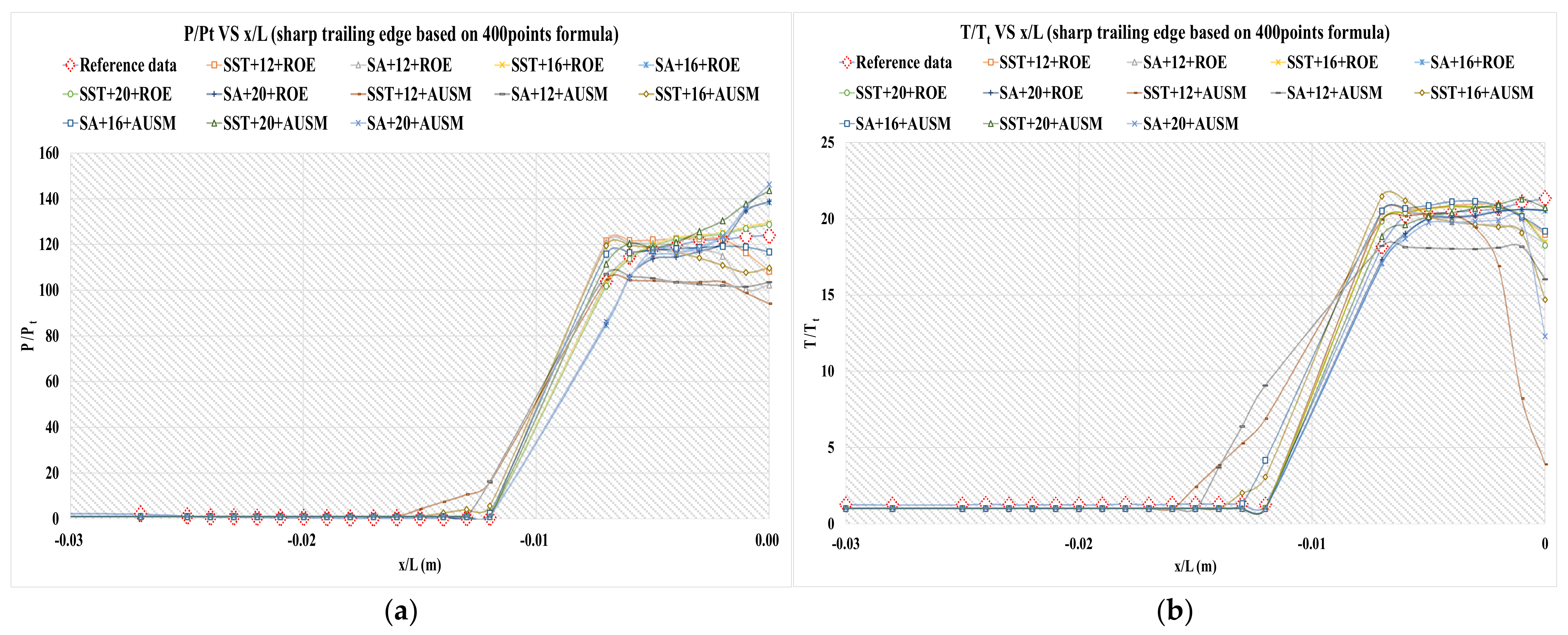
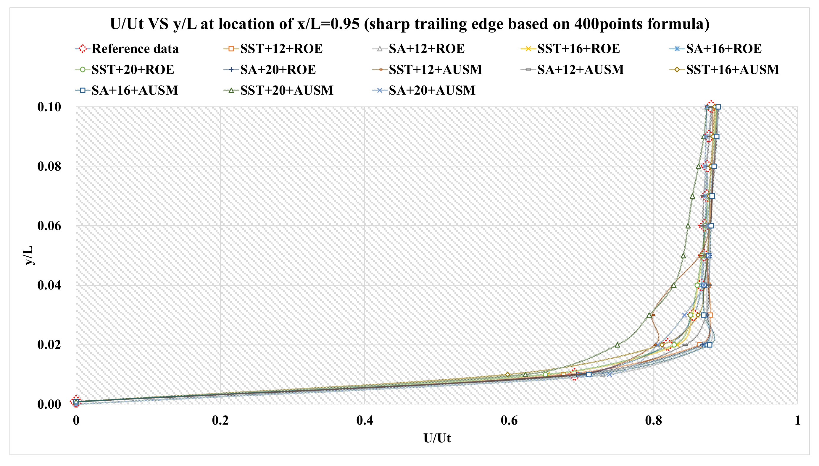
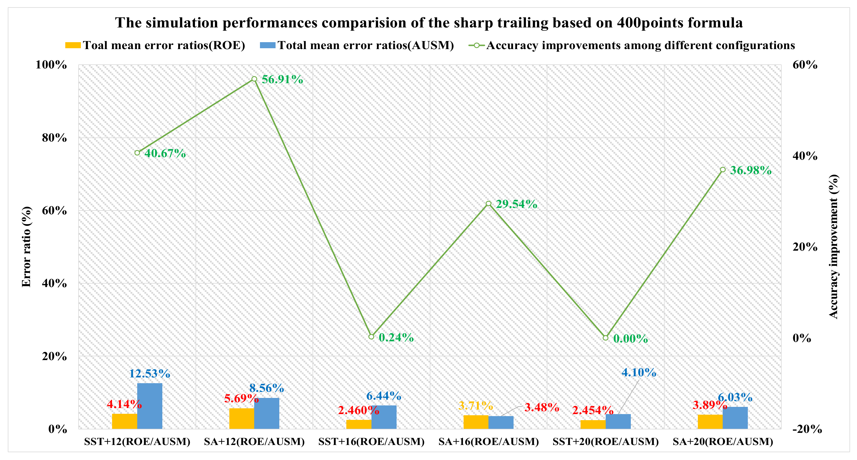
3.1.6. Results of the Sharp Trailing Edge Based on Definition Formula Applying 400 Points

Figure 20 and Figure 21 depict the distributions of P/Pt, T/Tt, and U/Ut of reference data and numerical data and the mean error ratios are presented in Table 17. Then the optimal total mean error ratios under different configurations are confirmed, as shown in Figure 22, which are highlighted in red. As to the far-field distance, the finest results for three distances are 4.14%, 2.46%, and 2.454%. As to the turbulence model, the minimum result of SST is 2.454%, and that of SA is 3.48%. As to the flux type, ROE has a minimum total mean error ratio of 2.454%, and that of AUSM is 3.48%. In conclusion, through the comparison among optimal performances of all configurations, SST + 20 m combined with ROE has the preferred result, and the value is 2.454% and the relevant accuracy growths are 40.67%, 56.91%, 0.24%, 29.54%, and 36.98%.
Table 17. The mean error ratios of P/Pt, T/Tt, and U/Ut of the sharp trailing edge based on 400 points.
Simulation
Configurations
Mean Error Ratios under Different Configurations
ROEAUSM
P/PtT/TtU/UtP/PtT/TtU/Ut
SST + 12 m6.02%4.72%1.66%13.60%22.17%1.83%
SA + 12 m8.66%6.36%2.06%12.65%12.06%0.95%
SST + 16 m2.21%4.08%1.09%7.75%9.69%1.89%
SA + 16 m6.96%2.86%1.32%3.66%4.98%1.81%
SST + 20 m2.06%4.22%1.08%6.48%1.71%4.10%
SA + 20 m7.35%2.74%1.59%7.52%9.22%1.35%

3.2. Far-Field Distance

Similar to the Section 3.1, combined with the six NACA0012 models, two turbulence models and two flux types, the following simulation configurations are obtained: SST + blunt (ROE/AUSM), SA + blunt (ROE/AUSM), SST + NACA4 (ROE/AUSM), SA + NACA4 (ROE/AUSM), SST + 132 points (ROE/AUSM), SA + 132 points (ROE/AUSM), SST + 200 points (ROE/AUSM), SA + 200 points (ROE/AUSM), SST + 264 points (ROE/AUSM), SA + 264 points (ROE/AUSM), SST + 400 points (ROE/AUSM), and SA + 400 points (ROE/AUSM). For each far-field distance, applying the parameters described in Table 8, twenty-four numerical simulations are performed, based on the results of which the related error ratios are calculated and the optimal performance is confirmed.

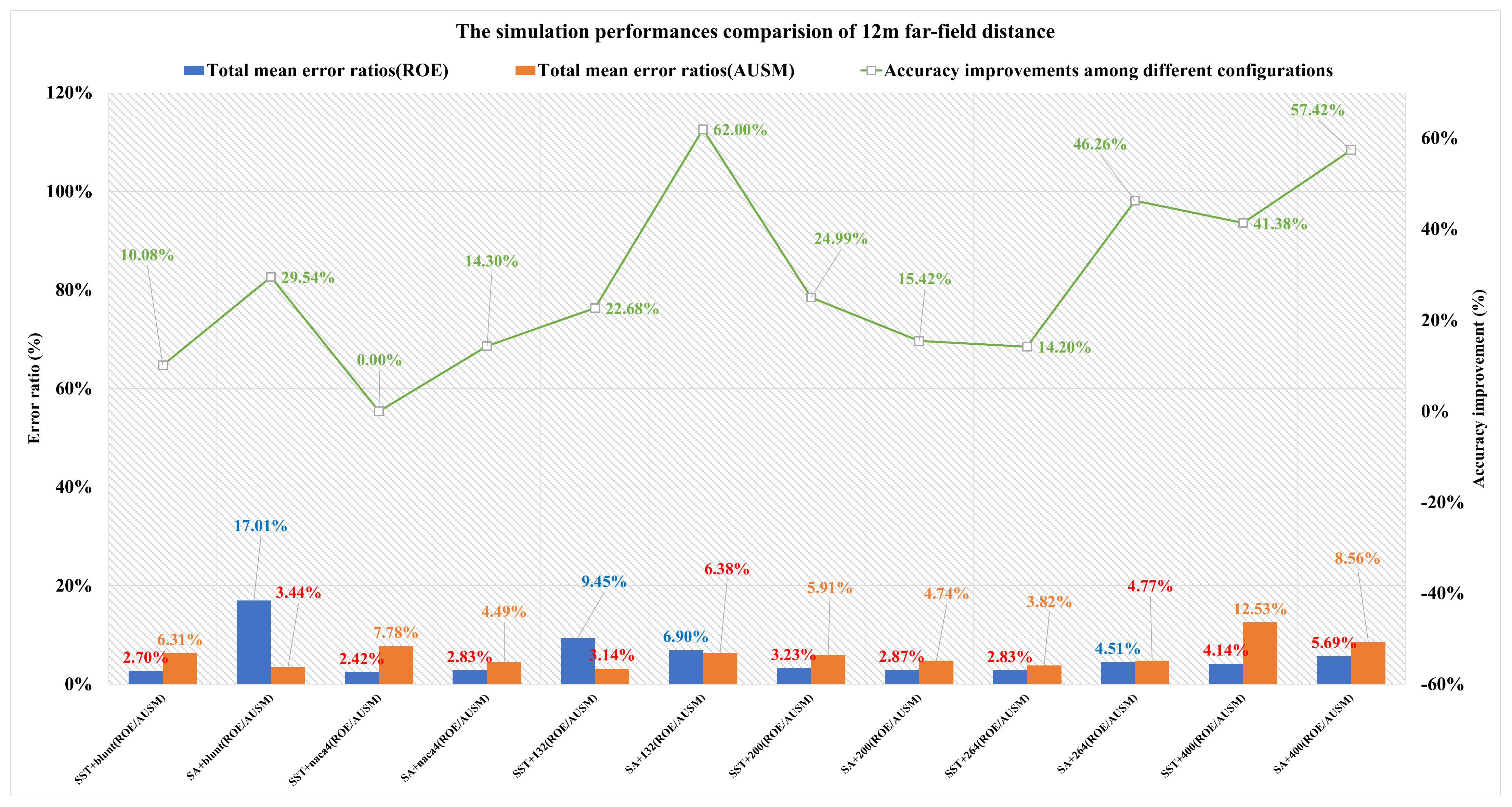
3.2.1. Results of 12 m Far-Field Distance

Figure 23 shows the distributions of P/Pt and T/Tt, and Table 18 provides the mean errors. The optimal total mean error ratios under different configurations are displayed in Figure 24, which are highlighted in red. For the NACA0012 model, the preferred results of the six models are 2.7%, 2.42%, 3.14%, 2.87%, 2.83%, and 4.14% in turn. For the turbulence model, SST has a minimum value of 2.42%, and that of SA is 2.83%. For the flux type, the best performance of ROE is 2.42%, and that of AUSM is 3.14%. Therefore, the configuration of SST + NACA4 combined with ROE behaves the best; the optimal value is 3.12% and the corresponding accuracy improvements are 10.08%, 29.54%, 14.3%, 22.68%, 62%, 24.99%, 15.42%, 14.2%, 46.26%, 41.38%, and 57.42%.

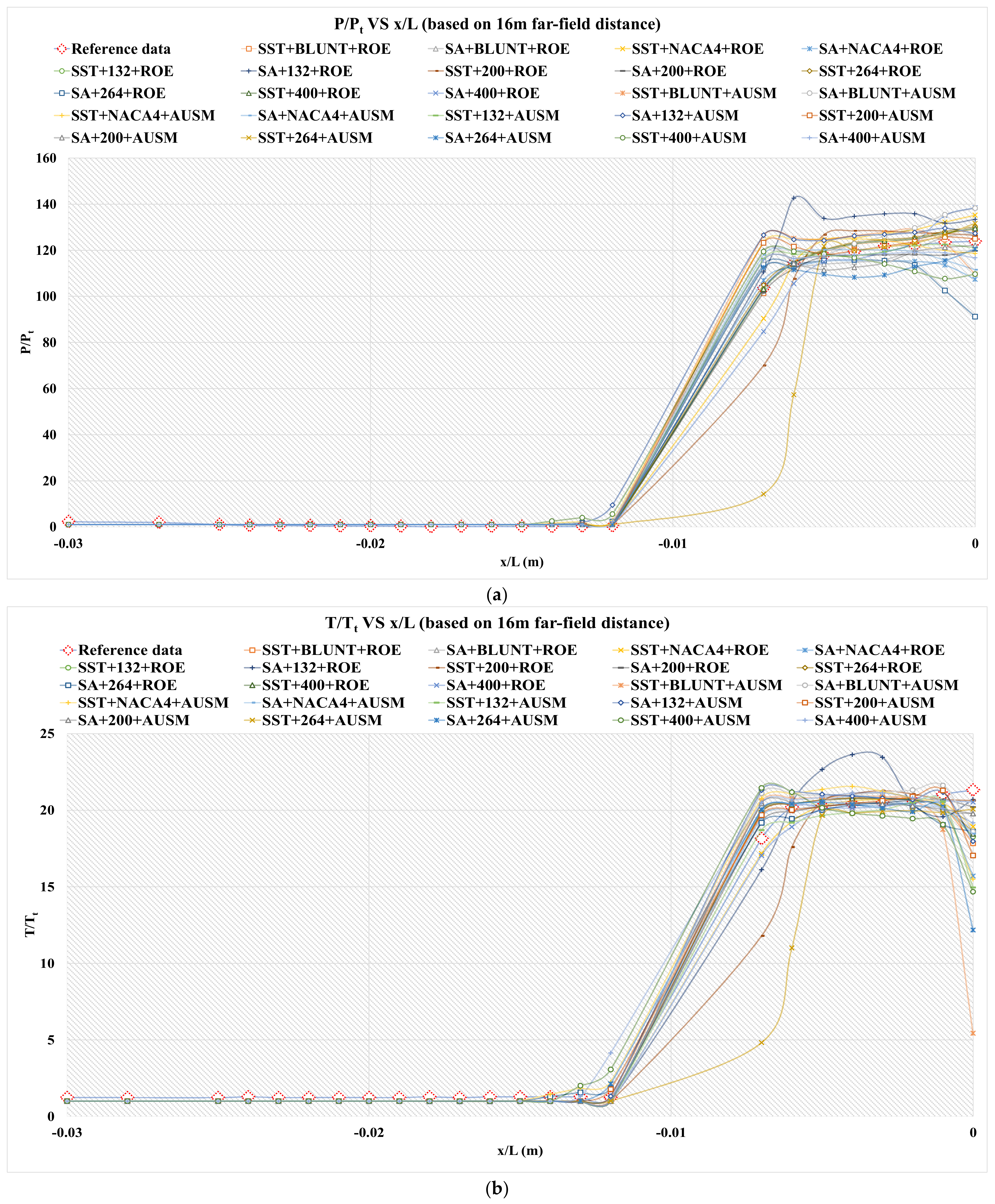
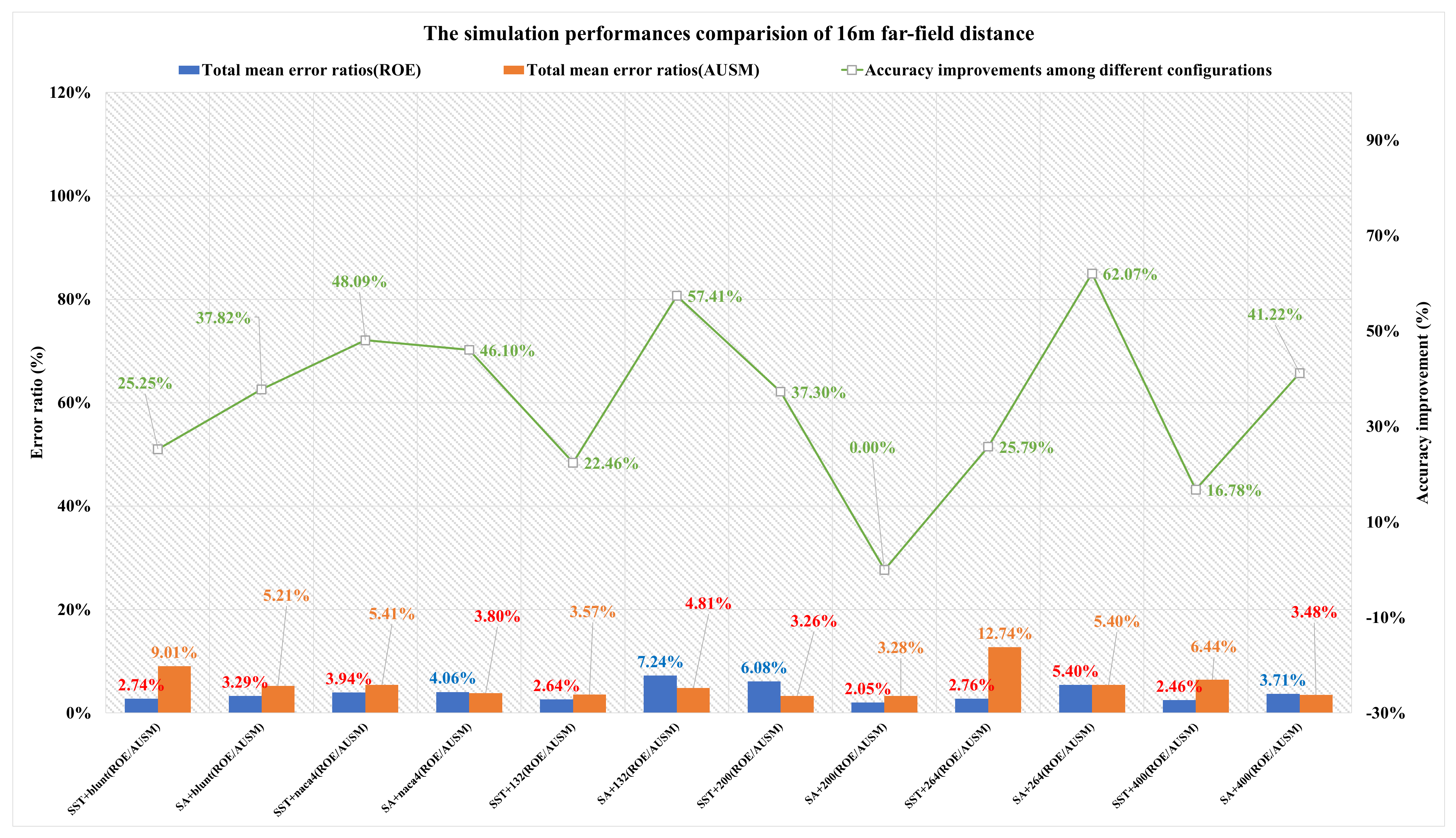
3.2.2. Results of 16 m Far-Field Distance

The distributions of P/Pt and T/Tt are presented in Figure 25, and the mean error ratios are contained in Table 19. The total mean error ratios under different configurations are calculated and the optimal results are highlighted in red in Figure 26. In terms of the NACA0012 model, the related finest performances are 2.74%, 3.8%, 2.64%, 2.05%, 2.76%, and 2.46%. In terms of the turbulence model, the optimal result of SST is 2.46%, and that of SA is 2.05%. In terms of the flux type, the optimal result of ROE is 2.05%, and that of AUSM is 3.26%. In general, we could conclude that SA + 200 points, combined with ROE, is the optimal configuration. The minimum total error ration is 2.05% and the relative accuracy gains are 25.25%, 37.82%, 48.09%, 46.10%, 22.46%, 57.41%, 37.3%, 25.79%, 62.07%, 16.78%, and 41.22%.

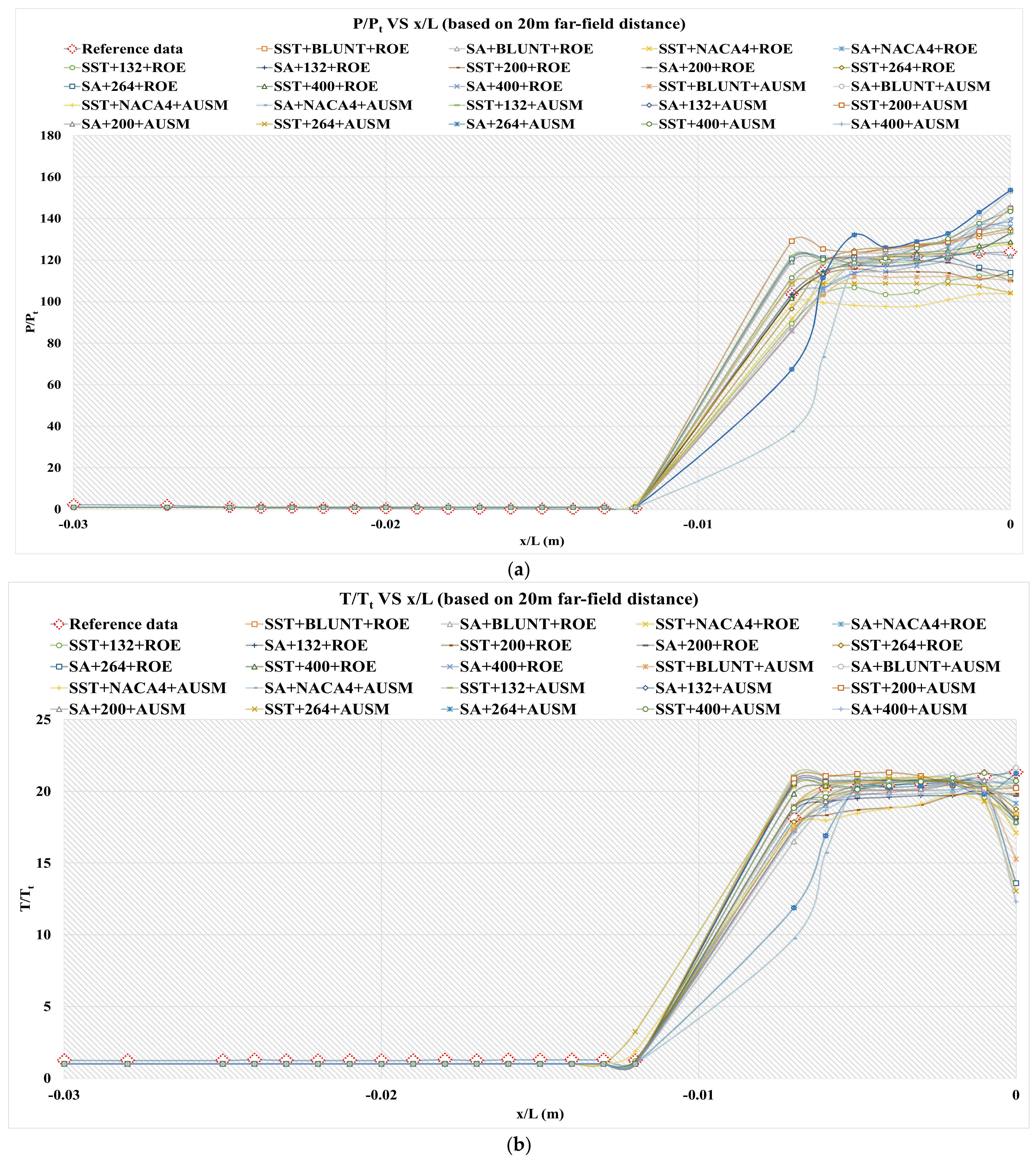
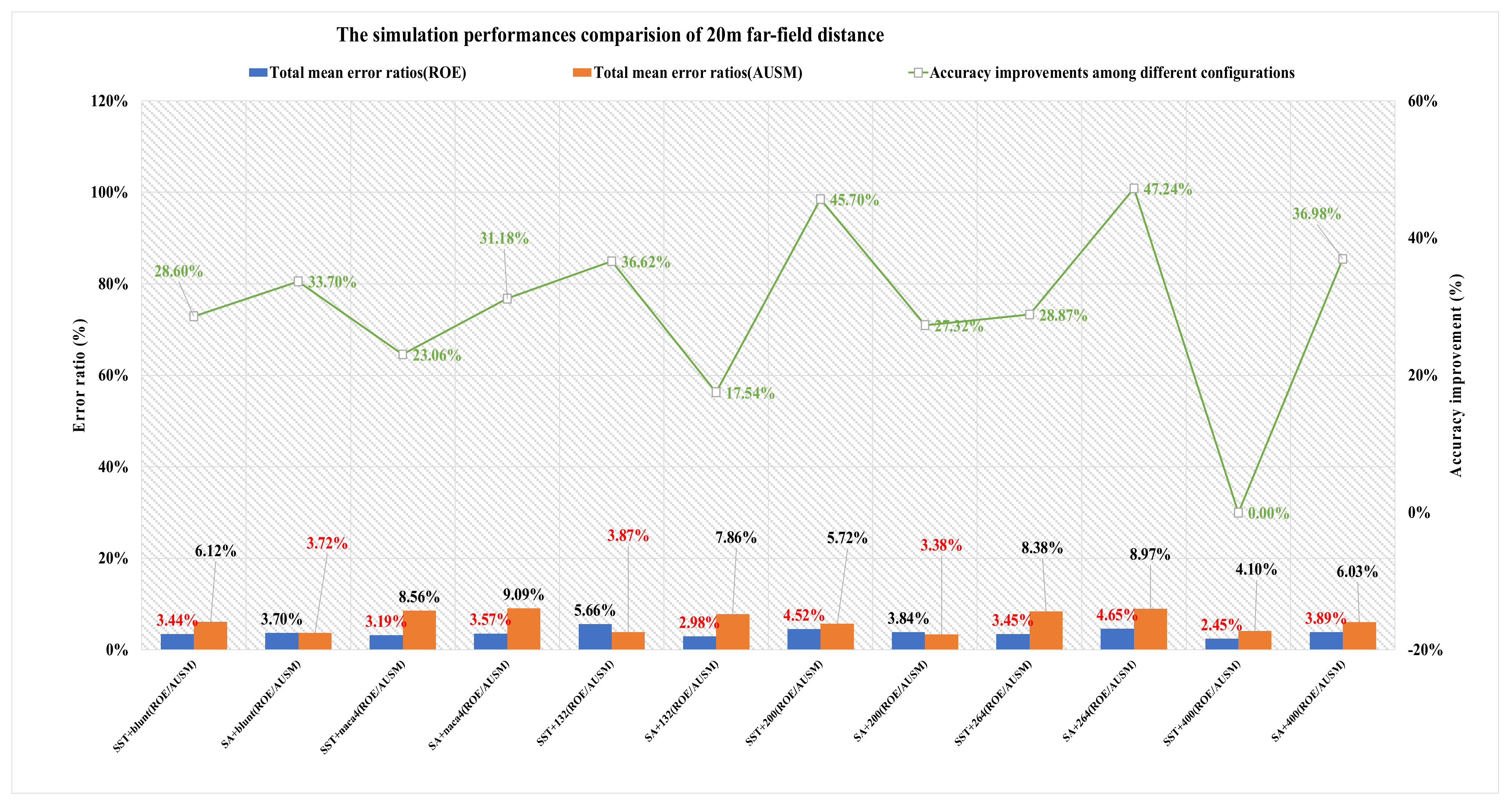
3.2.3. Results of 20 m Far-Field Distance

Figure 27 demonstrates the distributions of P/Pt and T/Tt, and Table 20 illustrates the mean error ratios. Figure 28 provides the optimal total mean error ratios under different configurations, which are highlighted in red. As for the NACA0012 model, the best results are 3.44%, 3.19%, 2.98%, 3.38%, 3.45%, and 2.45%. As for the turbulence model, the minimum results are 2.45% and 2.98%. As for the flux type, the smallest value of ROE is 2.45%, and that of AUSM is 3.38%. Through the results comparison among all the configurations, the optimal total mean error ratio is 2.45%, which is gained by the SST + 400 points combined with ROE, and the relevant accuracy advances are 28.6%, 33.7%, 23.06%, 31.18%, 36.62%, 17.54%, 45.7%, 27.32%, 28.87%, 47.24%, and 36.98% in order.

3.3. Turbulence Model

Similar to the previous sections, based on the six NACA0012 models, three far-field distances, and two flux types, the below simulation configurations are obtained: 12 m + blunt(ROE/AUSM), 16 m + blunt (ROE/AUSM), 20 m + blunt (ROE/AUSM), 12 m + NACA4 (ROE/AUSM), 16 m + NACA4 (ROE/AUSM), 20 m + NACA4 (ROE/AUSM), 12 m + 132 points (ROE/AUSM), 16 m + 132 points(ROE/AUSM), 20 m + 132 points (ROE/AUSM), 12 m + 200 points (ROE/AUSM), 16 m + 200 points (ROE/AUSM), 20 m + 200 points (ROE/AUSM), 12 m + 264 points (ROE/AUSM), 16 m + 264 points (ROE/AUSM), 20 m + 264 points (ROE/AUSM), 12 m + 400 points (ROE/AUSM), 16 m + 400 points (ROE/AUSM), and 20 m + 400 points (ROE/AUSM). Then for each turbulence model, combined with the parameters of Table 8, thirty-six simulations are performed. By comparing the mean error ratios under different configurations, we confirm the corresponding optimal result and the simulation configuration.

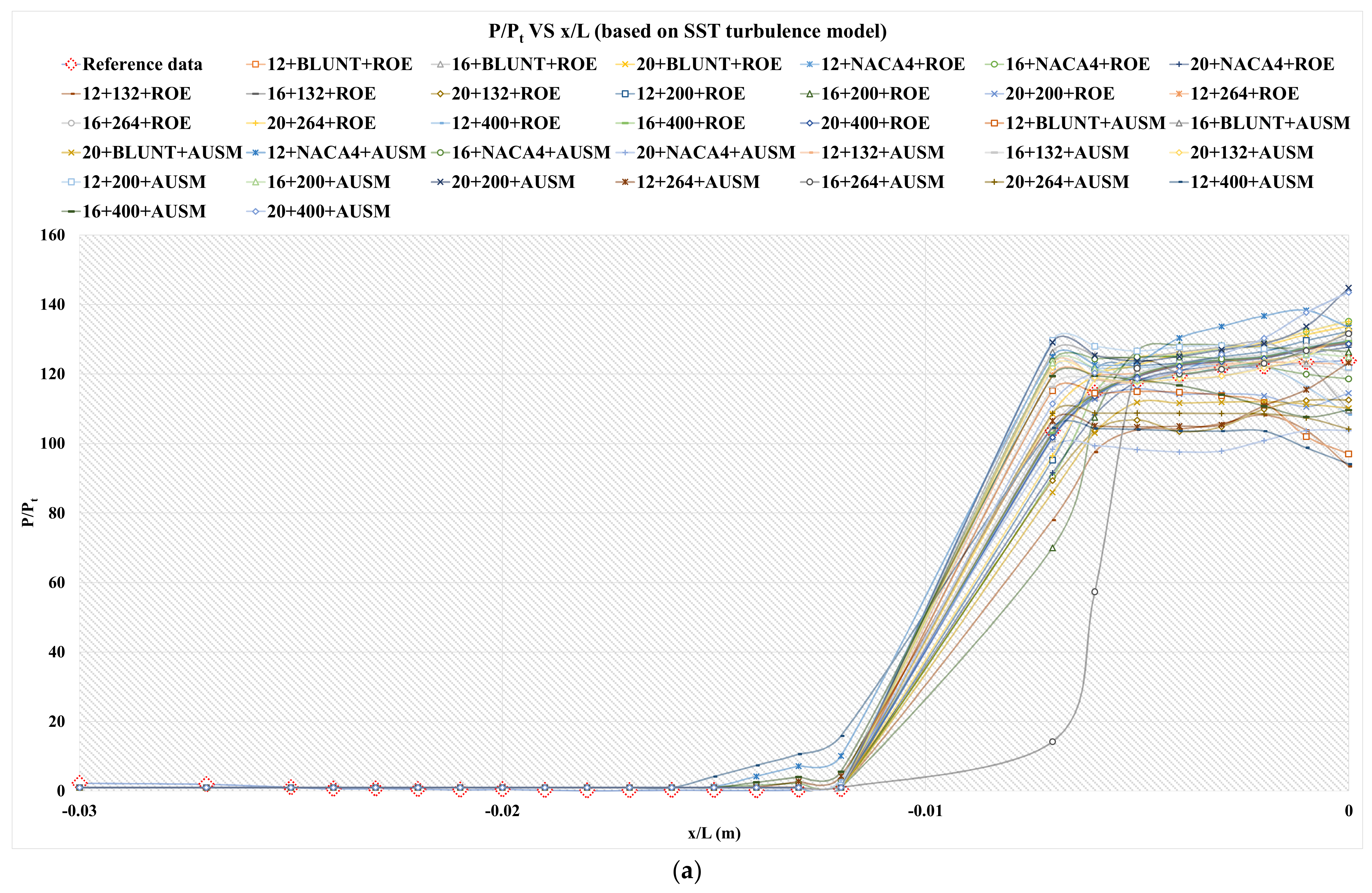
3.3.1. Results of SST k-Omega

The distributions of P/Pt and T/Tt are presented in Figure 29, and the mean error ratios are illustrated in Table 21. We then determine the total mean error ratios under different configurations, and the optimal results are highlighted in red in Figure 30. As to the far-field distance, the three distances have the following minimum results: 2.42%, 2.46%, and 2.454%. As for the NACA0012 model, the best performances are 2.7%, 2.42%, 2.64%, 3.23%, 2.76%, and 2.454% in order. As for the flux type, ROE has the optimal value of 2.42%, and that of AUSM is 3.14%. Therefore, the ideal configuration is 12 m + NACA4 combined with ROE. The optimal result is 2.42%, and the corresponding accuracy improvements are 10.24%, 11.62%, 29.58%, 38.63%, 24.11%, 22.82%, 8.32%, 37.49%, 25.12%, 25.87%, 46.44%, 14.36%, 12.26%, 29.84%, 41.48%, 1.61%, and 1.37%.

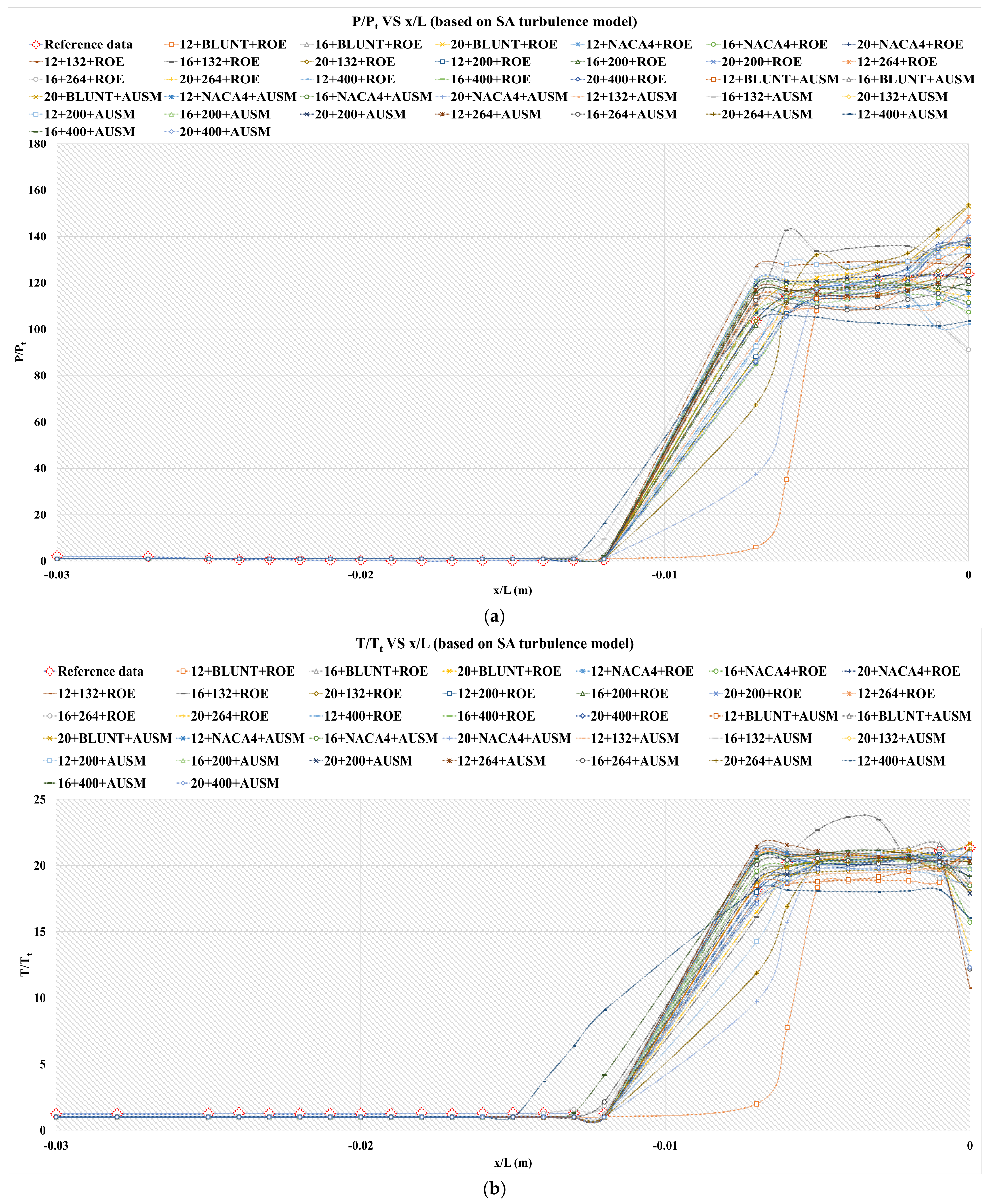
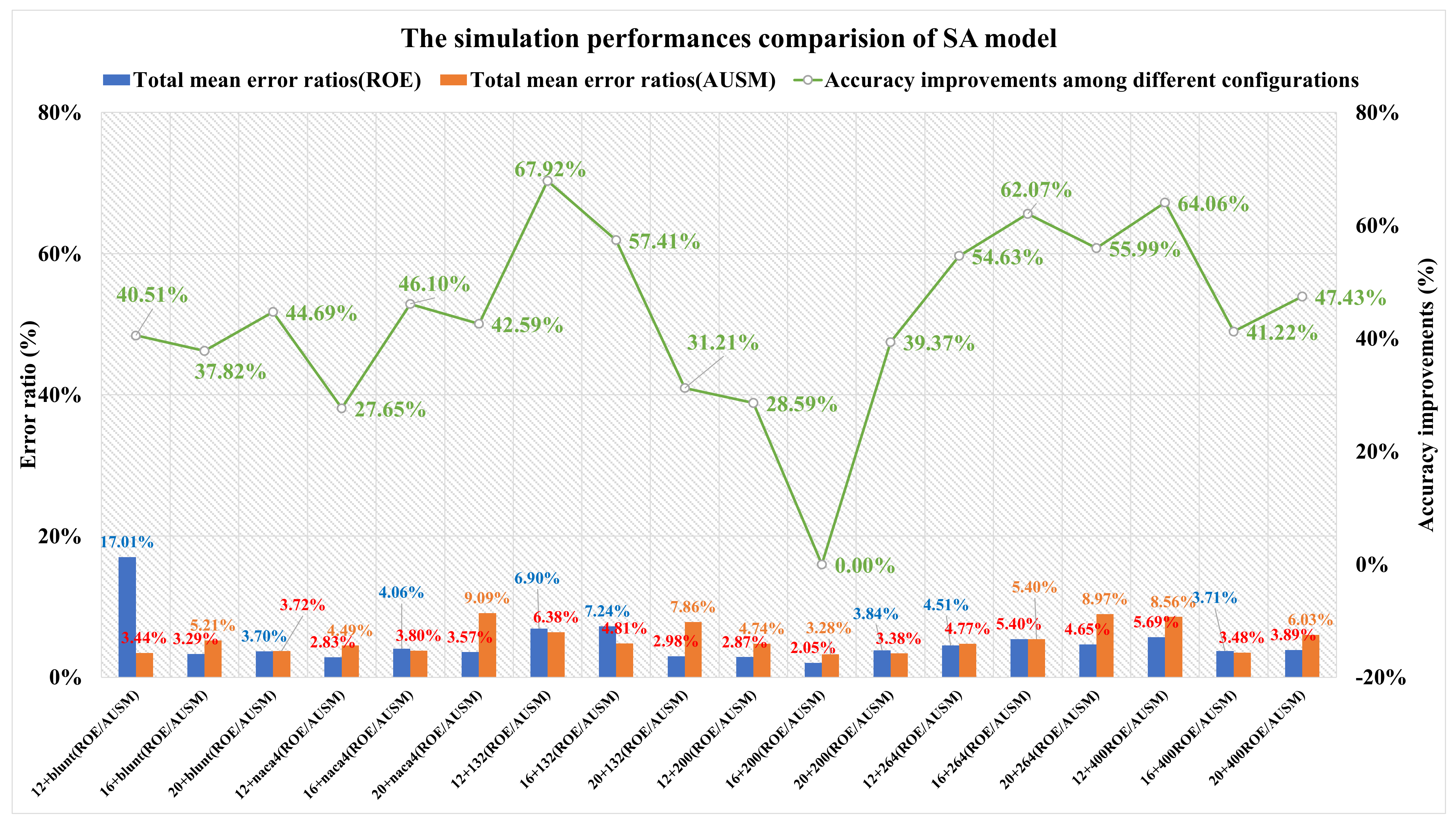
3.3.2. Results of Spalart–Allmaras

Figure 31 depicts the distributions of P/Pt and T/Tt, and Table 22 contains the mean error ratios. We then determine the total mean error ratios under different configurations and the optimal results are highlighted in red in Figure 32. As to the far-field distance, the following 2.83%, 2.05%, and 2.98% are the three preferred results. As for the NACA0012 model, the best performances are 3.29%, 2.83%, 2.98%, 2.05%, 4.51%, and 3.48% in order. As for the flux type, ROE has the optimal value of 2.05%, and that of AUSM is 3.28%. Therefore, the ideal configuration is 16 m + 200 points combined with ROE. The optimal result is 2.05%, and the related accuracy growths are 40.51%, 37.82%, 44.69%, 27.65%, 46.10%, 42.59%, 67.92%, 57.41%, 31.21%, 28.59%, 39.37%, 54.63%, 62.07%, 55.99%, 64.06%, 41.22%, and 47.43%.

3.4. Flux Type

Similar to the previous sections, adopting six NACA0012 models, three far-field distances, and two turbulence models, we have the following simulation configurations: SST + blunt (12/16/20 m), SA + blunt (12/16/20 m), SST + NACA4 (12/16/20 m), SA + NACA4 (12/16/20 m), SST + 132 points (12/16/20 m), SA + 132 points (12/16/20 m), SST + 200 points (12/16/20 m), SA + 200 points (12/16/20 m), SST + 264 points (12/16/20 m), SA + 264 points (12/16/20 m), SST + 400 points(12/16/20 m), and SA + 400 points (12/16/20 m). For each flux type, adopting parameters provided in Table 8, thirty-six simulations are performed. Based on the numerical results, we calculate the mean error ratios and confirm the optimal configuration.

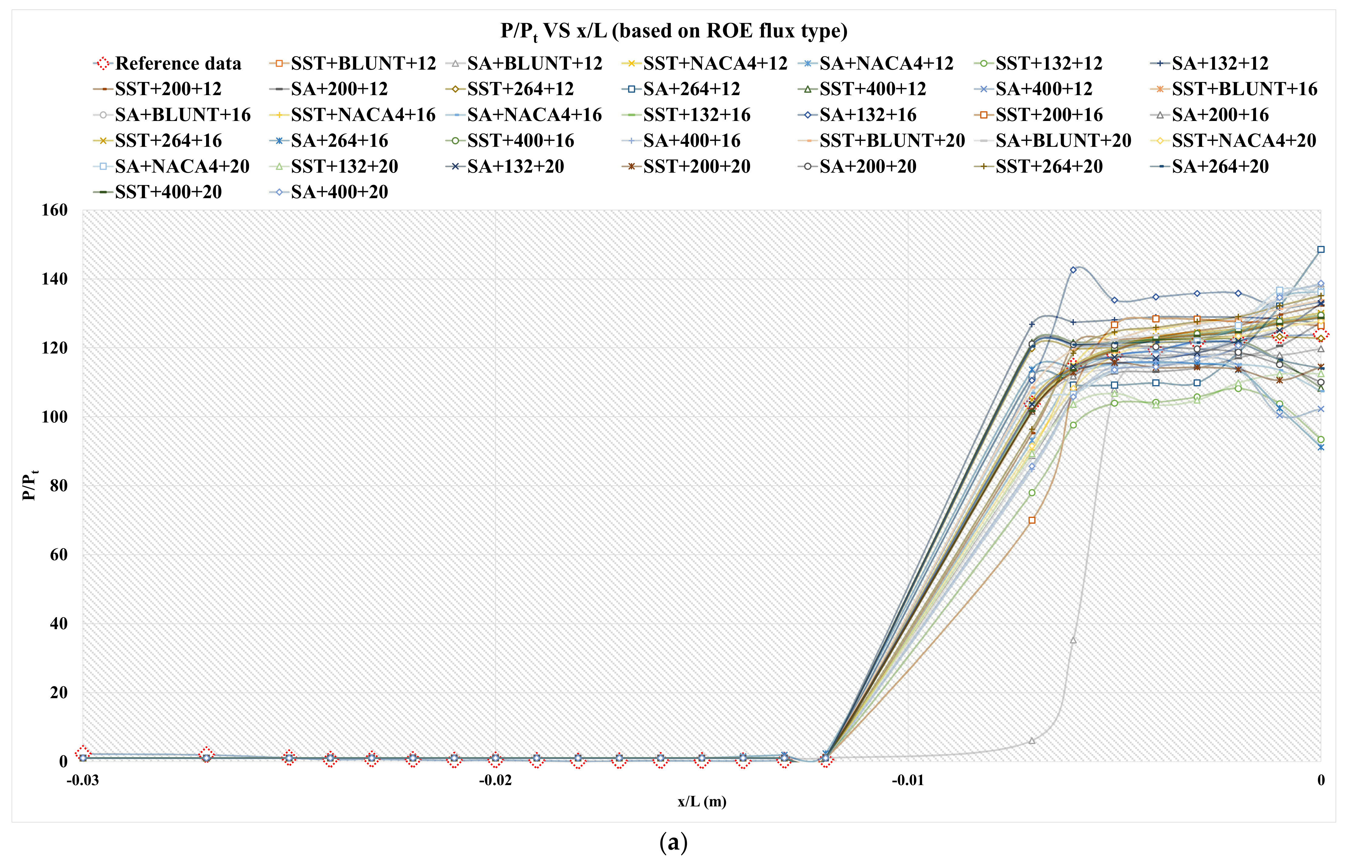
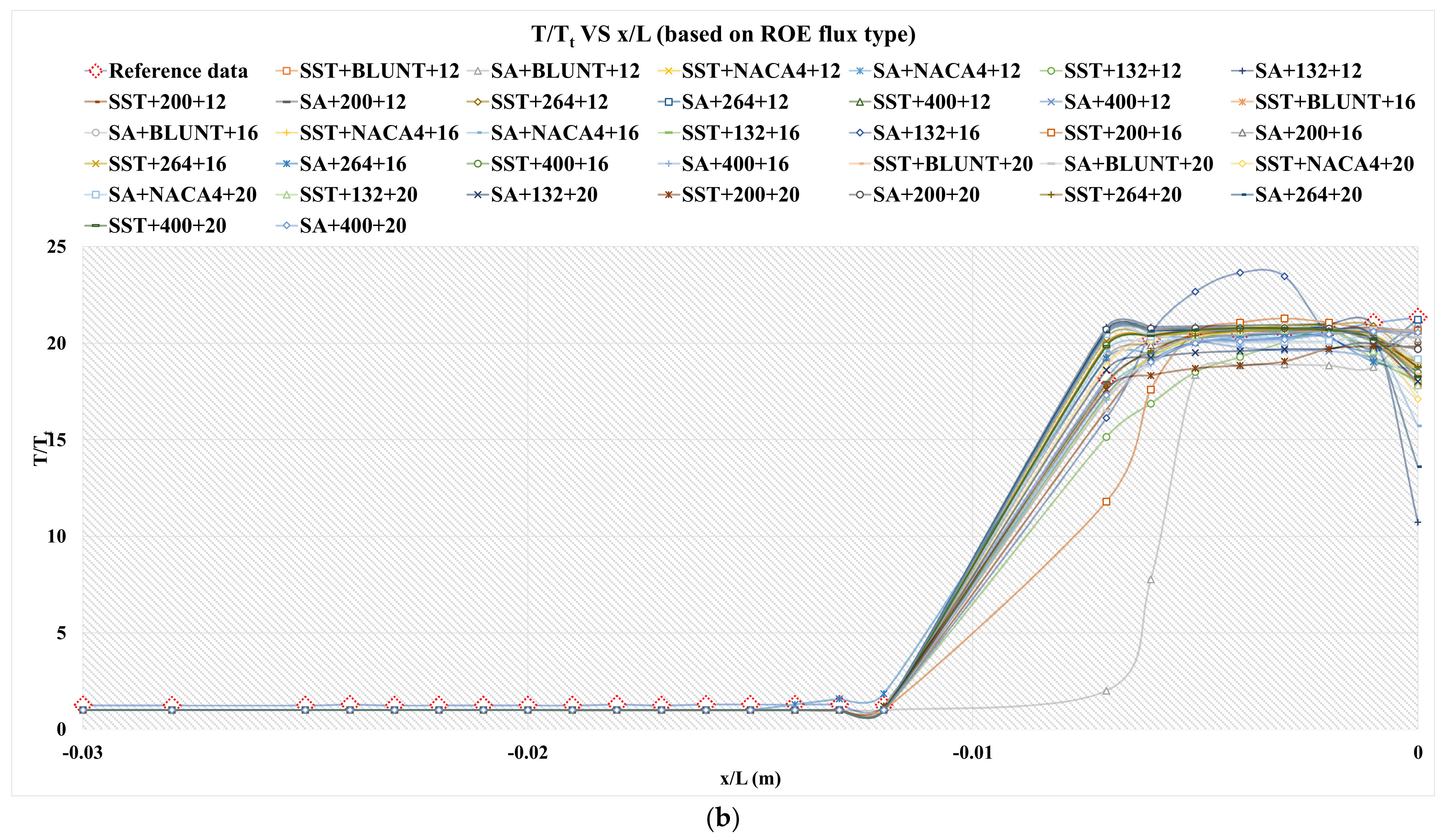
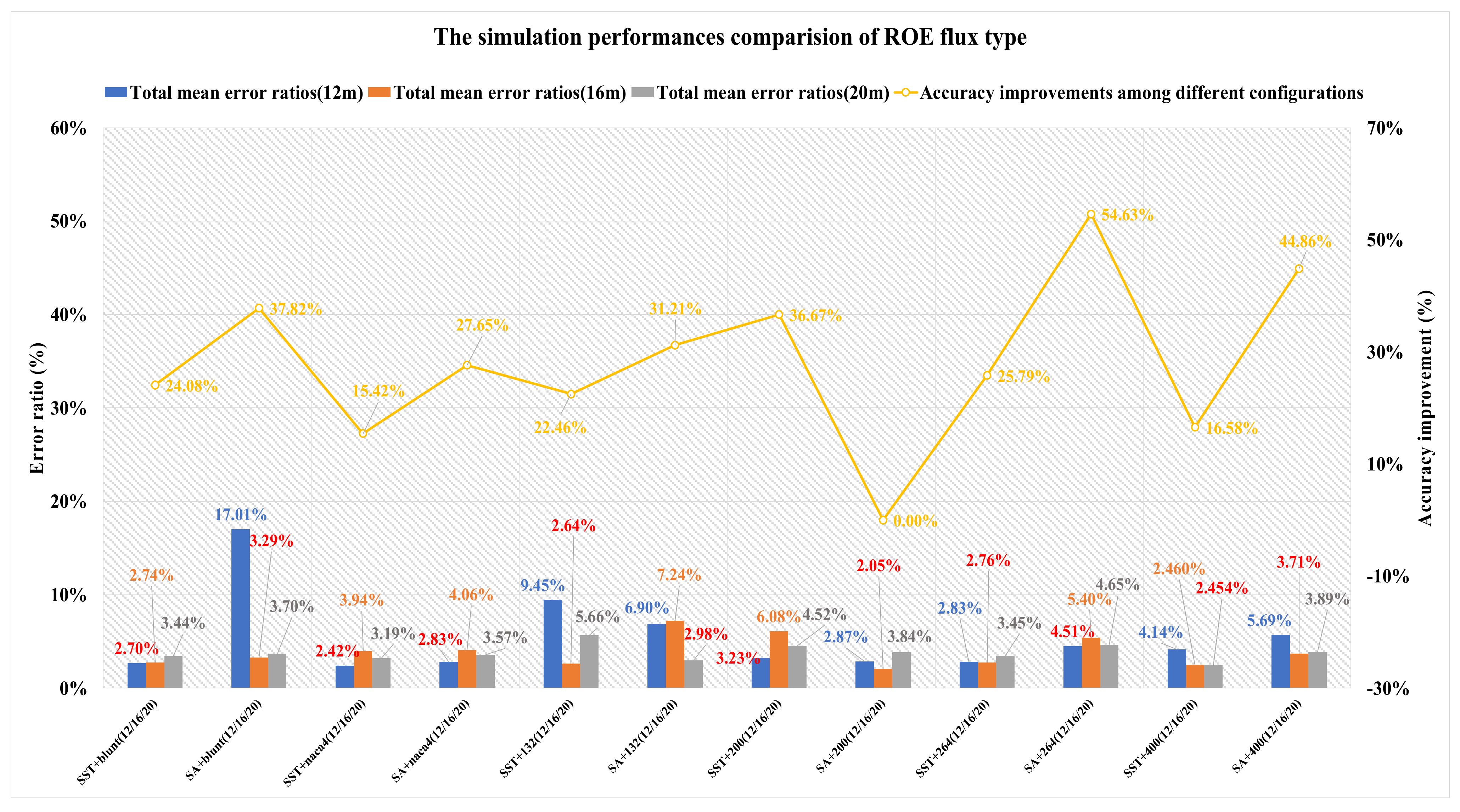
3.4.1. Results of ROE Flux Type

The distributions of P/Pt and T/Tt are presented in Figure 33, and the mean error ratios are illustrated in Table 23. Based on the above results, the optimal total mean error ratios under different configurations are confirmed, as shown in Figure 34, which are highlighted in red. For the turbulence model, SST has the best performance of 2.42%, and that of SA is 2.05%. For the NACA0012 model, the minimum results are 2.70%, 2.42%, 2.64%, 2.05%, 2.76%, and 2.454% in order. For the far-field distance, the finest values of the three distances are 2.42%, 2.05%, and 2.454%. In conclusion, the optimal configuration is SA + 200 points combined with 16 m far-field distance, the total mean error ratio of which is 2.05% and is obtained by comparison performances for all configurations. The corresponding accuracy improvements are 24.08%, 37.82%, 15.42%, 27.65%, 22.46%, 31.21%, 36.67%, 25.79%, 54.63%, 16.58%, and 44.86%.

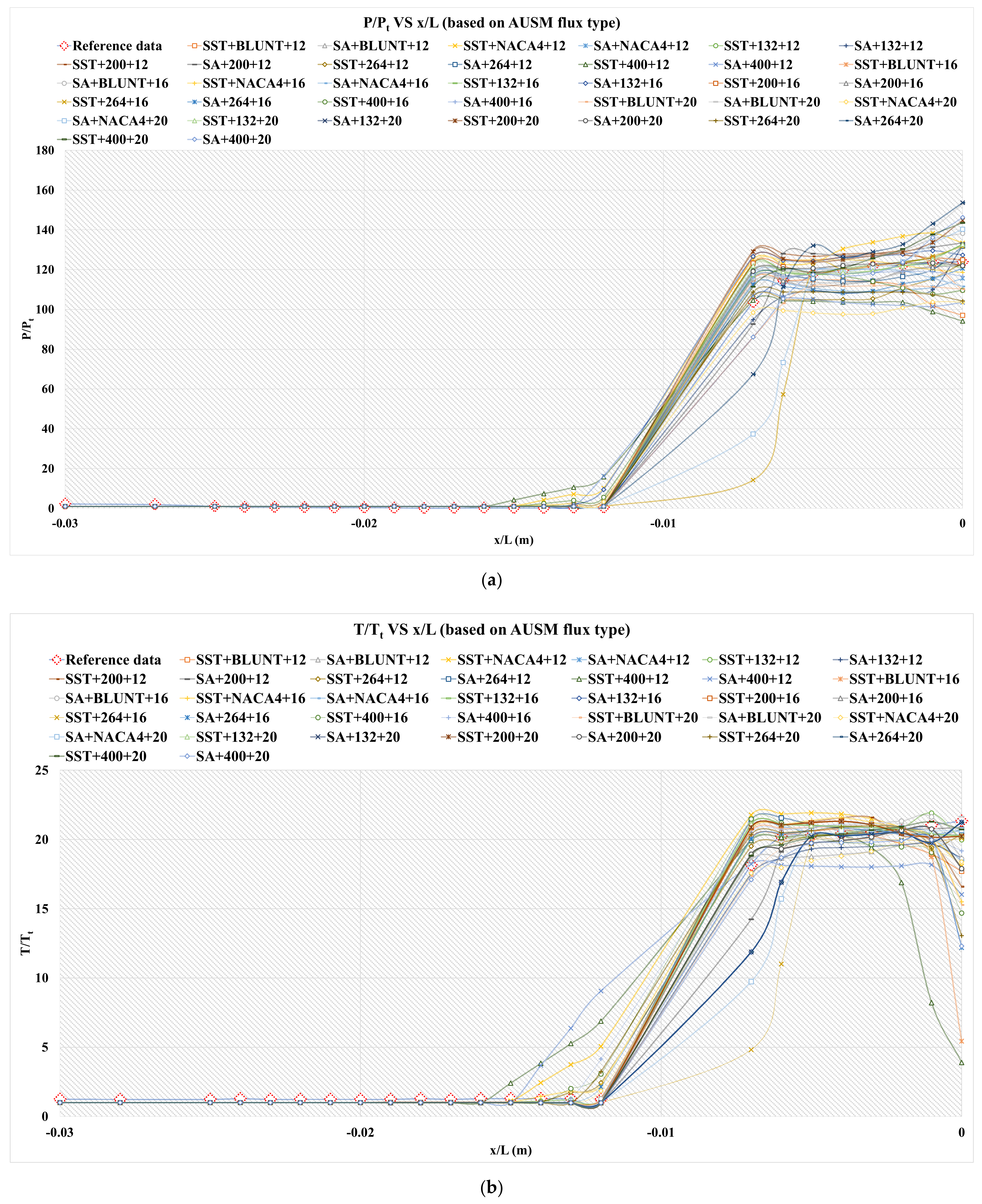
3.4.2. Results of AUSM Flux Type

Figure 35 demonstrates the distributions of P/Pt and T/Tt, and Table 24 illustrates the corresponding mean error ratios. We then determine the mean error ratios under different configurations, which are depicted in Figure 36, and the optimal results are highlighted in red. In terms of the turbulence model, SST has the best result of 3.14%, and that of SA is 3.28%. For the NACA0012 model, the finest performances are 3.44%, 3.80%, 3.14%, 3.26%, 3.82%, and 3.48% in order. For the far-field distance, the minimum values of the three distances are 3.14%, 3.26%, and 3.38%. Through the performance comparison among all the configurations, the optimal configuration is SST + 132 points combined with a 12 m far-field distance, and the total mean error ratio is 3.14%. The relative accuracy growths are 48.75%, 8.87%, 42.02%, 17.42%, 34.75%, 3.94%, 4.33%, 17.96%, 34.24%, 23.45%, and 9.95% in order.

3.5. Discussion

The optimal total error ratios and the related prediction accuracy changes of the six NACA0012 models are illustrated in Figure 37. For the trailing edge shape, except for the designed sharp trailing edge based on the definition formula adopting 264 points, the blunt trailing edge performs worse than the sharp trailing edge and the related accuracy declines are 11.41%, 2.14%, 31.73%, and 9.88% in order. The inappropriate selection of the trailing edge shape would cause a fairly big error and the maximum prediction accuracy decrease degree could reach 31.73%. Next, considering the three modeling methods, the optimal result of the Airfoil tools method is 2.7%, and those of the NACA4 generator and definition formula are 2.42% and 2.05% in order. Moreover, the definition formula could provide the best performance, the accuracy improvements of which compared with the other two methods are 24.08% and 15.42%. It is worth noting that though the definition formula could obtain the minimum total error ratio, except for the condition of the definition formula adopting 200 points, NACA4 behaves better. So, the choice between NACA4 and the definition formula is determined by the adopted data points. Further, considering the influences of data point source adopted in the definition formula and the number on the simulation accuracy, for the 132 data points sourced from the Airfoil tools, with the number doubled to 264, the prediction accuracy drops and the accuracy decrement is 4.55%. For the 200 data points sourced from the NACA4 generator, the prediction accuracy also drops and the decline degree is 19.71% with the number doubled to 400. Hence, the increase of the data point number actually decreases the prediction accuracy instead of improving it. Among the applied four numbers of data points, the optimal results of 200 and 400 data points are 2.05% and 2.454%, which are better than those of 132 and 264 data points. Compared with the other three, the corresponding improvements of 200 data points are calculated and the values are 22.46%, 25.79%, and 16.58%, respectively. As a result, data points from NACA4 have a better performance than that of the data points from Airfoil tools and the addition of the data point number is not directly correlated with the calculation accuracy. In conclusion, we should give priority to choosing the definition formula to design the sharp trailing edge and adopting the 200 data points supplied by NACA4.
The optimal total error ratios of far-field distances, turbulence models, flux types, and the related accuracy improvements are presented in Figure 38. Considering the far-field distance, the prediction accuracy is increased as the far-field distance increases from 12L to 16L, and the accuracy improvement is 15.42%, while the accuracy drops as the further increase from 16L to 20L, and the decline degree is 19.88%. We could conclude that the performance of 16 m far-field distance is preferred and the related accuracy improvements are 15.42% and 16.58%, in turn. Therefore, the boosts of the far-field distance may not undoubtedly result in a rise in simulation accuracy but result in a decline, and the far-field distance of 16L is recommended. Further, considering the turbulence model, at the far-field distances of 12L and 20L, SST behaves better than SA and the related accuracy improvements are 14.30% and 17.54%. But at a far-field distance of 16L, the superior result is obtained by the SA and this is the finest value of the turbulence model. Hence, the turbulence model choice is related to the far-field distance, and the SA turbulence model should be preferentially considered. As to the flux type, as shown in Figure 38, ROE could achieve a better performance than that of AUSM, as the minimum improvement is 22.68% and the maximum improvement is 37.3%. Therefore, the ROE flux type is suggested.
Based on the results from Section 3.1 to Section 3.4, the optimal mean error ratios under different configurations are provided in Table 25. It is summarized that in terms of the blunt trailing edge based on the Airfoil tools, SST + 12 m combined with ROE is the recommended simulation configuration and the optimal results are (1.97%, 4.52%, 1.6%). In terms of the sharp trailing edge based on NACA4, the preferred configuration is SST + 12 m combined with ROE and the results are (2.28%, 3.96%, 1.04%). In terms of the definition formula, applying 200 points sourced from NACA4 combined with SA + 16 m + ROE could achieve the optimal results of (2.54%, 1.86%, 1.74%). Moreover, attention should be paid that improper parameter selection may lead to a large decline in the simulation accuracy. As shown in Table 22, the maximum decline degrees of the four parameter types, which are highlighted in bold, are 31.73%, 19.88%, 18.45%, and 53.2% in order. In particular, an inappropriately adopted sharp trailing edge modeling method could lead to an accuracy decline of 34.76%. The above conclusions suggest that the inappropriate sharp trailing edge modeling method may introduce more error ratio than the inappropriate trailing edge shape and the unsuitable flux type pick would bring the largest drop degree in prediction accuracy.

4. Conclusions

According to the reference data of Ref [17], under hypersonic speed, a detailed parameters influence of trailing edge shapes, far-field distances, turbulence models, and flux types on the simulation prediction accuracy of the compressible external flow field characterized by NACA0012 airfoil is discussed in this paper. The appropriate grid strategy and number method are confirmed in Section 2. Through comparisons among numerical mean error ratios, the internal relationships between the prediction accuracy and the abovementioned parameters are discussed in detail in Section 3. In particular, the trailing edge shape, the related modeling methods, the source, and quantity of the adopted data point dependencies are discussed in Section 3.5. Compared with the influence analysis discussions under incompressible external flow field at the AOA is 0° in Ref [3], the following conclusions could be drawn:
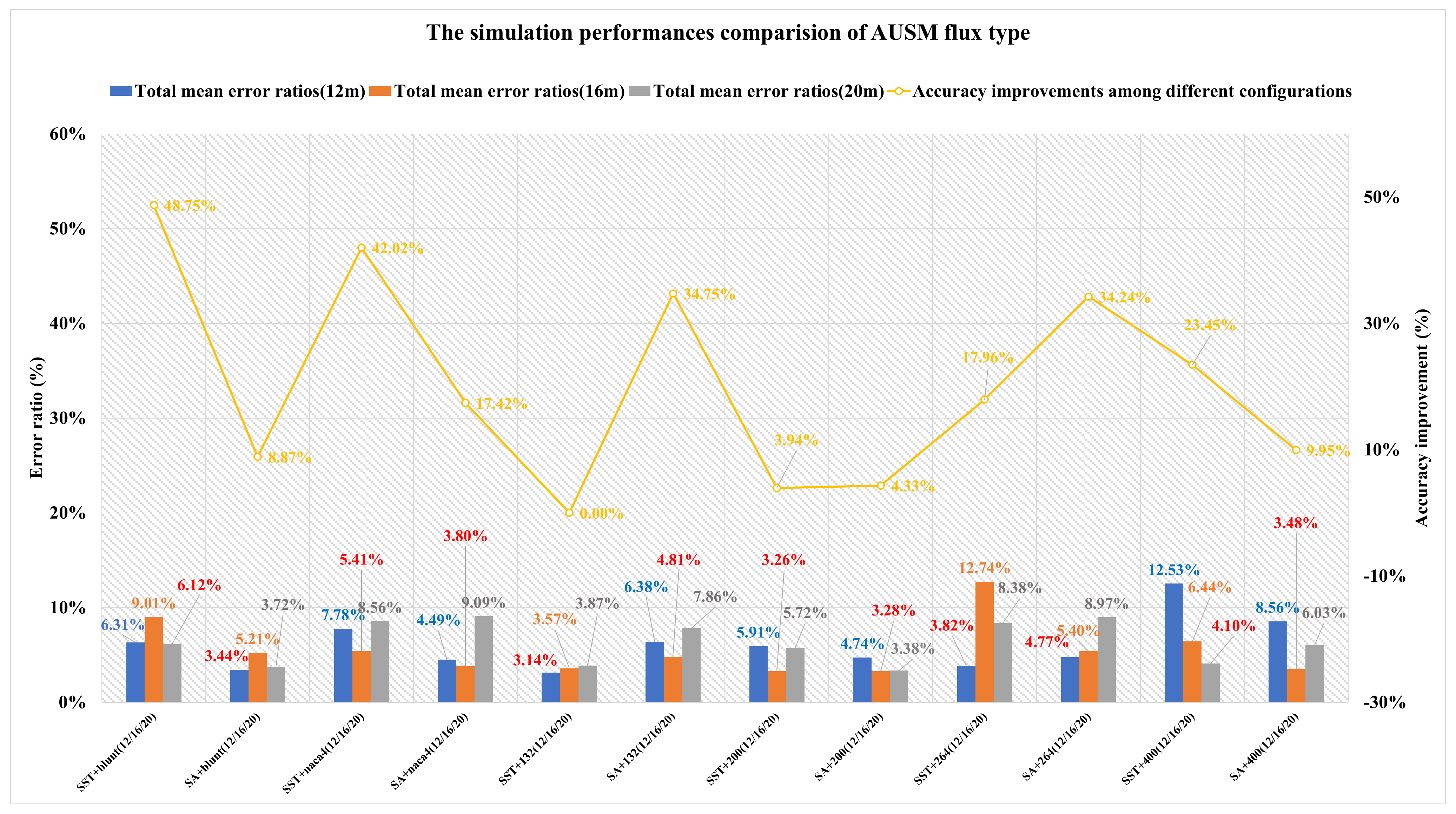
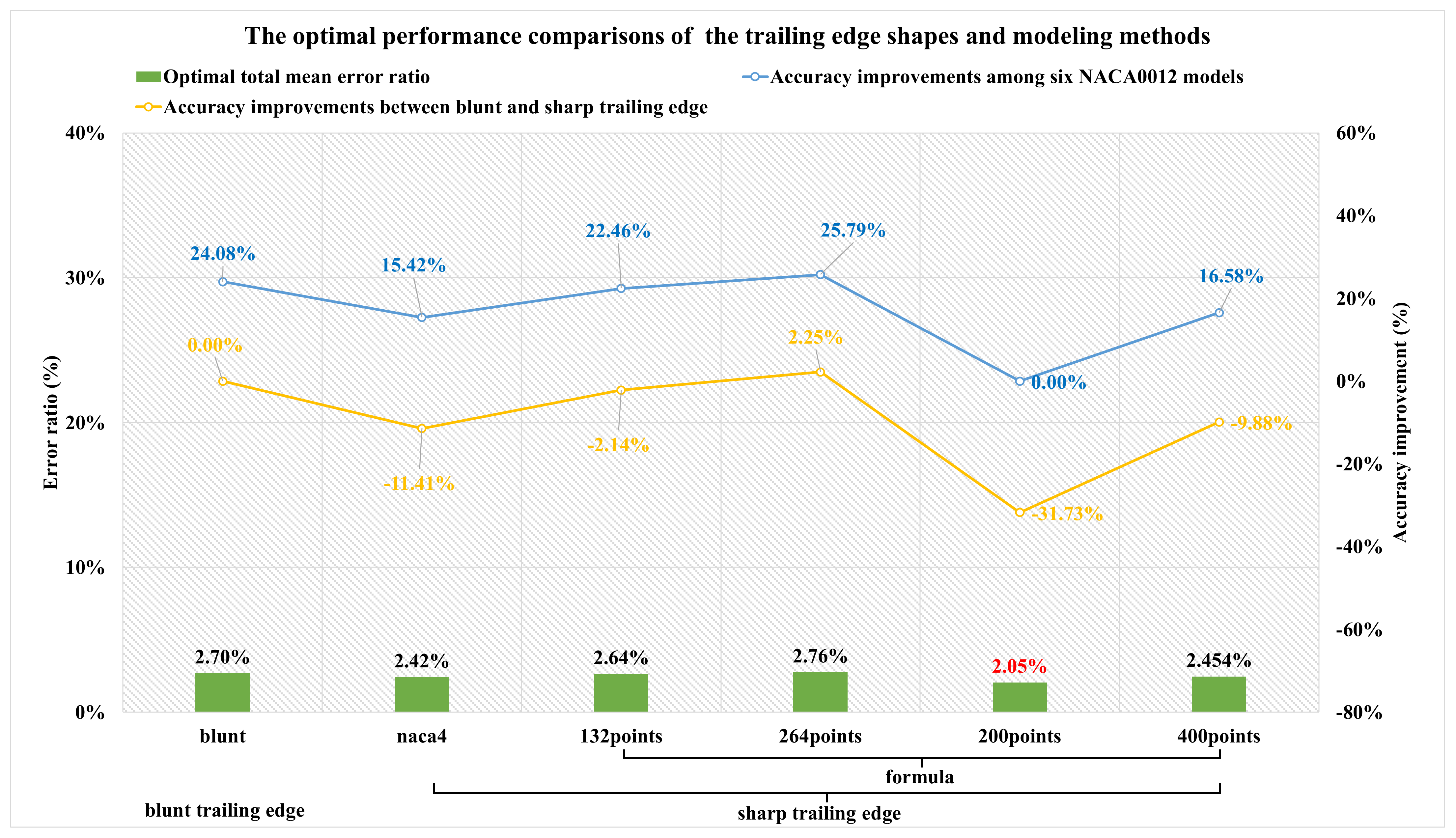
  • Unlike under incompressible external flow field, as to the trailing edge shape selection, the improper sharp trailing edge design could bring a larger error ratio than that of the blunt trailing edge shape. A similar situation exists for the modeling methods selection, in particular for the choice between the NACA4 and the definition formula. Except in a case where the definition formula adopts 200 points, NACA4 is preferred to establish the NACA0012 airfoil. Further, whether the adopted data points are from Airfoil tools or the NACA4 generator, the increase in the number of data points could not bring about an improvement in calculation accuracy. As to the far-field distance, the maximum far-field distance could not lead to the minimum simulation error ratio. Specifically, the numerical accuracy is promoted with the far-field distance increases from 12L to 16L; then that is decreased with the further from 16L to 20L and a 16L far-field distance is suggested. As to the turbulence model, the performance of SA adopting second-order upwind modified turbulent viscosity is better than that of SA adopting first-order. As for the flux type, the calculation accuracy of the ROE flux type is better than that of the AUSM flux type, and the unsuitable flux type selection could cause maximum accuracy loss.
  • Despite the rise of the far-field distance, which would result in the aspect ratio addition on the condition it could be limited within a reasonable range, the simulation accuracy could be promoted as the far-field increases. The suggests that the maximum aspect ratio value is within 4800 and the minimum determinant value is above 0.82.
  • In this paper, as shown in Table 25, the sharp trailing edge based on 200 points definition formula, a 16L far-field distance, SA turbulence model, and ROE flux type is the preferred simulation configuration and the optimal mean error ratios are (2.54%, 1.86%, 1.74%).

Author Contributions

Conceptualization, L.Y. and G.Z.; methodology, L.Y. and G.Z.; investigation, L.Y.; formal analysis, L.Y.; resources, L.Y. and G.Z.; validation, L.Y.; visualization, L.Y.; writing—original draft preparation, L.Y.; writing-review and editing, L.Y. and G.Z. All authors have read and agreed to the published version of the manuscript.

Funding

This research received no external funding.

Institutional Review Board Statement

Not applicable.

Informed Consent Statement

Not applicable.

Data Availability Statement

Data is contained within the article.

Acknowledgments

The researcher would like to express gratitude for the support received from family and colleagues.

Conflicts of Interest

The authors declare no conflict of interest.

References

  1. Chen, F.; Liu, H.; Zhang, S. Time-adaptive loosely coupled analysis on fluid–thermal–structural behaviors of hypersonic wing structures under sustained aeroheating. Aerosp. Sci. Technol. 2018, 78, 620–636. [Google Scholar] [CrossRef]
  2. Qu, F.; Kong, W.; Sun, D.; Bai, J. Shock-stable flux scheme for predicting aerodynamic heating load of hypersonic airliners. Sci. China Ser. G Phys. Mech. Astron. 2019, 62, 984711. [Google Scholar] [CrossRef]
  3. Yang, L.; Zhang, G. Analysis of Influence of Different Parameters on Numerical Simulation of NACA0012 Incompressible External Flow Field under High Reynolds Numbers. Appl. Sci. 2022, 12, 416. [Google Scholar] [CrossRef]
  4. Sadikin, A.; Yunus, N.A.M.; Abd Hamid, S.A.; Ismail, A.E.; Salleh, S.; Ahmad, S.; Rahman, M.N.A.; Mahzan, S.; Ayop, S.S. A comparative study of turbulence models on aerodynamics characteristics of a NACA0012 airfoil. Int. J. Integr. Eng. 2018, 10, 134–137. [Google Scholar] [CrossRef] [Green Version]
  5. Zheng, X.; Liu, Z.; Yang, Y.; Lei, J.-C.; Li, Z.-X. Research on Climb-cruise Global Trajectory Optimization for RBCC Hypersonic Vehicle. Missiles Space Veh. 2018, 47, 1–8. (In Chinese) [Google Scholar]
  6. Vassberg, J.C.; Jameson, A. In pursuit of grid convergence for two-dimensional Euler solutions. J. Aircr. 2010, 47, 1152–1166. [Google Scholar] [CrossRef] [Green Version]
  7. Diskin, B.; Thomas, J.L.; Rumsey, C.L.; Schwoppe, A. Grid-convergence of Reynolds-averaged Navier-stokes solutions for benchmark flows in two dimensions. AIAA J. 2016, 54, 2563–2588. [Google Scholar] [CrossRef]
  8. Devi, P.B.; Paulson, V.; Madhanraj, V.; Shah, D.A. Heat transfer and temperature effects on a dimpled NACA0012 airfoil with various angles of attack. Int. J. Ambient Energy 2018, 39, 783–786. [Google Scholar] [CrossRef]
  9. Devi, P.B.; Shah, D.A. Effect of square dimples on the temperature distribution and heat transfer coefficient of an NACA0012 airfoil. Int. J. Ambient Energy 2019, 40, 754–757. [Google Scholar] [CrossRef]
  10. Joseph, D.R.; Devi, P.B.; Gopalsamy, M. Investigation on effect of square dimples on NACA0012 airfoil with various Reynolds numbers. Int. J. Ambient Energy 2021, 42, 397–402. [Google Scholar] [CrossRef]
  11. Bekka, N.; Bessaih, R.; Sellam, M.; Chpoun, A. Numerical study of heat transfer around the small scale airfoil using various turbulence models. Numer. Heat Transf. Part A Appl. 2009, 56, 946–969. [Google Scholar] [CrossRef]
  12. Hinz, D.F.; Alighanbari, H.; Breitsamter, C. Influence of heat transfer on the aerodynamic performance of a plunging and pitching NACA0012 airfoil at low Reynolds numbers. J. Fluids Struct. 2013, 37, 88–99. [Google Scholar] [CrossRef]
  13. Cheng, J.; Lai, Y.; Wang, L.; Wu, H.; Li, L. Study on the icing characteristics of typical wind turbine. J. Hebei Univ. Sci. Technol. 2019, 40, 9–14. (In Chinese) [Google Scholar] [CrossRef]
  14. Kang, H.K. Numerical simulation of Aeroacoustic Noise at Low Mach Number Flows by Using the Finite Difference Lattice Boltzmann Method. J. Adv. Mar. Eng. Technol. 2004, 28, 717–727. [Google Scholar]
  15. Kang, H.K.; Lee, Y.H.; Tsutahara, M.; Shikata, K.; Kim, E.R.; Kim, Y.T. Computation OF Aerodynamic Sounds AT Low Mach Numbers Using Finite Difference Lattice Boltzmann Method. Korean Soc. Comput. Fluids Eng. 2005, 10, 8–15. [Google Scholar]
  16. Rattanasiri, P.; Perrin, R. Influence of the Wavelength of Cut-In Sinusoidal Trailing Edge Shape to the Aerodynamics Characteristic of the Airfoil. IOP Conf. Ser. Mater. Sci. Eng. 2020, 886, 012020. [Google Scholar] [CrossRef]
  17. Perrin, R.; Rattanasiri, P.; Lamballais, E.; Yooyen, S. Influence of the trailing edge shape on the aerodynamic characteristics of an airfoil at low Re number using RANS. IOP Conf. Ser. Mater. Sci. Eng. 2020, 886, 012021. [Google Scholar] [CrossRef]
  18. Singh, J.P. Evaluation of Jameson-Schmidt-Turkel dissipation scheme for hypersonic flow computations. J. Aircraft. 1996, 33, 286–290. [Google Scholar] [CrossRef]
  19. Delery, J.; Coet, M.C. Experiments on Shock-Wave/Boundary-Layer Interactions Produced by Two-Dimensional Ramps and Three-Dimensional Obstacles. In Hypersonic Flows for Reentry Problems Désidéri; Glowinski, J.A., Périaux, R.J., Eds.; Springer: Berlin/Heidelberg, Germany, 1990. [Google Scholar]
  20. Kussoy, M.I.; Horstman, C.C. Documentation of Two- and Three-Dimensional Hypersonic Shock Wave/Turbulent Boundary Layer Interaction Flows. In NASA Technical Memorandum 101075; NASA Ames Research Center: Moffett Field, CA, USA, 1989. [Google Scholar]
  21. Yang, L.; Zhang, G. An Effective Simulation Scheme for Predicting the Aerodynamic Heat of a Scramjet-Propelled Vehicle. Appl. Sci. 2021, 11, 9344. [Google Scholar] [CrossRef]
  22. ICEM. CFD Hexa 2D Airfoil Meshing. Available online: https://www.youtube.com/watch?v=EknKVAJGEJ8&t=58s (accessed on 9 May 2022).
  23. Ansys, Inc. Ansys Fluent Theory Guide; Ansys, Inc.: Canonsburg, PA, USA, 2021. [Google Scholar]
  24. Schlichting, H.; Gersten, K. Boundary-Layer Theory, 7th ed.; Springer: Berlin/Heidelberg, Germany, 1979; ISBN 0070553343. [Google Scholar]
  25. Smirnov, N.N.; Penyazkov, O.G.; Sevrouk, K.L.; Nikitin, V.F.; Stamov, L.I.; Tyurenkova, V.V. Detonation onset following shock wave focusing. Acta Astronaut. 2017, 135, 114–130. [Google Scholar] [CrossRef]
  26. Launder, B.E.; Spalding, D.B. The Numerical Computation of Turbulent Flow. Comput. Methods Appl. Mech. Eng. 1974, 3, 269–289. [Google Scholar] [CrossRef]
  27. Menter, F.R. Two-equation eddy-viscosity turbulence models for engineering applications. AIAA J. 1994, 32, 1598–1605. [Google Scholar] [CrossRef] [Green Version]
  28. Spalart, P.; Allmaras, S. A one-equation turbulence model for aerodynamic flows. In Proceedings of the 30th Aerospace Sciences Meeting and Exhibit, Reno, NV, USA, 6–9 January 1992; p. 439. [Google Scholar] [CrossRef]
  29. Weiss, J.M.; Smith, W.A. Preconditioning applied to variable and constant density flows. AIAA J. 1995, 33, 2050–2057. [Google Scholar] [CrossRef]
  30. Roe, P.L. Characteristic-based schemes for the Euler equations. Annu. Rev. Fluid Mech. 1986, 18, 337–365. [Google Scholar] [CrossRef]
  31. Liou, M.S. A sequel to ausm: Ausm+. J. Comput. Phys. 1996, 129, 364–382. [Google Scholar] [CrossRef]
  32. Li, J.; Yan, C.; Ke, L.; Zhang, S. Research on scheme effect of computational fluid dynamics in aerothermal. J. Beijing Univ. Aeronaut. Astronaut. 2003, 11, 1022–1025. (In Chinese) [Google Scholar] [CrossRef]
  33. Ansys, Inc. Ansys Fluent User’s Guide; Ansys, Inc.: Canonsburg, PA, USA, 2021. [Google Scholar]
  34. Wilcox, D.C. Turbulence Modeling for CFD; DCW Industries, Inc.: La Canada, CA, USA, 1998. [Google Scholar]
  35. Barth, T.; Jespersen, D. The design and application of upwind schemes on unstructured meshes. In Proceedings of the 27th Aerospace Sciences Meeting, Reno, NV, USA, 9–12 January 1989; p. 366. [Google Scholar] [CrossRef]
Figure 1. (a) Six NACA0012 airfoil models; (b) Close view of different models.
Applsci 12 06083 g001
Figure 2. (a) Grid division of the sharp trailing edge; (b) Grid division of the blunt trailing edge.
Applsci 12 06083 g002
Figure 3. (a) Close view of meshes near the WALL region; (b) Close view of meshes near the sharp trailing edge.
Applsci 12 06083 g003
Figure 4. (a) Close view of meshes near the WALL region; (b) Close view of meshes near the blunt trailing edge.
Applsci 12 06083 g004
Figure 5. (a) Distributions of P/Pt of the blunt trailing edge; (b) Distributions of T/Tt of the blunt trailing edge.
Applsci 12 06083 g005
Figure 6. Distributions of U/Ut of the blunt trailing edge at location of x/L = 0.95.
Applsci 12 06083 g006
Figure 7. Comparison of the simulation performances of the blunt trailing edge under different sim-ulation configurations.
Applsci 12 06083 g007
Figure 8. (a) Distributions of P/Pt of sharp trailing edge based on NACA 4-digital; (b) Distributions of T/Tt of sharp trailing edge based on NACA 4-digital.
Applsci 12 06083 g008
Figure 9. Distributions of U/Ut of the sharp trailing edge based on NACA4 at location of x/L = 0.95.
Applsci 12 06083 g009
Figure 10. Comparison of the simulation performances of the sharp trailing edge based on NACA4 under different simulation configurations.
Applsci 12 06083 g010
Figure 11. (a) Distributions of P/Pt based on 132 points definition formula; (b) Distributions of T/Tt based on 132 points definition formula.
Applsci 12 06083 g011
Figure 12. Distributions of U/Ut of the sharp trailing edge based on 132 points formula at location of x/L = 0.95.
Applsci 12 06083 g012
Figure 13. Comparison of the simulation performances of the sharp trailing edge based on 132 points formula under different simulation configurations.
Applsci 12 06083 g013
Figure 14. (a) Distributions of P/Pt of sharp trailing edge based on 264 points formula; (b) Distributions of T/Tt of sharp trailing edge based on 264 points formula.
Applsci 12 06083 g014
Figure 15. Distributions of U/Ut of the sharp trailing edge based on 264 points formula at location of x/L = 0.95.
Applsci 12 06083 g015
Figure 16. Comparison of the simulation performances of the sharp trailing edge based on 264points formula under different simulation configurations.
Applsci 12 06083 g016
Figure 17. (a) Distributions of P/Pt of sharp trailing edge based on 200 points formula; (b) Distributions of T/Tt of sharp trailing edge based on 200 points formula.
Applsci 12 06083 g017
Figure 18. Distributions of U/Ut of the sharp trailing edge based on 200 points formula at location of x/L = 0.95.
Applsci 12 06083 g018
Figure 19. Comparison of the simulation performances of the sharp trailing edge based on 200 points formula under different simulation configurations.
Applsci 12 06083 g019
Figure 20. (a) Distributions of P/Pt of sharp trailing edge based on 400 points formula; (b) Distributions of T/Tt of sharp trailing edge based on 400 points formula.
Applsci 12 06083 g020
Figure 21. Distributions of U/Ut of the sharp trailing edge based on 400 points formula at location of x/L = 0.95.
Applsci 12 06083 g021
Figure 22. Comparison of the simulation performances of the sharp trailing edge based on 400 points formula under different simulation configurations.
Applsci 12 06083 g022
Figure 23. (a) Distributions of P/Pt of 12 m far-field distance; (b) Distributions of T/Tt of 12 m far-field distance.
Applsci 12 06083 g023
Figure 24. Comparison of the simulation performances of 12 m far-field distance under different simulation configurations.
Applsci 12 06083 g024
Figure 25. (a) Distributions of P/Pt of 16 m far-field distance; (b) Distributions of T/Tt of 16 m far-field distance.
Applsci 12 06083 g025
Figure 26. Comparison of the simulation performances of 16 m far-field distance under different simulation configurations.
Applsci 12 06083 g026
Figure 27. (a) Distributions of P/Pt of 20 m far-field distance; (b) Distributions of T/Tt of 20 m far-field distance.
Applsci 12 06083 g027
Figure 28. Comparison of the simulation performances of 20 m far-field distance under different simulation configurations.
Applsci 12 06083 g028
Figure 29. (a) Distributions of P/Pt of SST turbulence model; (b) Distributions of T/Tt of SST turbu-lence model.
Applsci 12 06083 g029aApplsci 12 06083 g029b
Figure 30. Comparison of the simulation performances of SST turbulence model under different simulation configurations.
Applsci 12 06083 g030
Figure 31. (a) Distributions of P/Pt of SA turbulence model; (b) Distributions of T/Tt of SA turbulence model.
Applsci 12 06083 g031
Figure 32. Comparison of the simulation performances of SA turbulence model under different sim-ulation configurations.
Applsci 12 06083 g032
Figure 33. (a) Distributions of P/Pt of ROE flux type; (b) Distributions of T/Tt of ROE flux type.
Applsci 12 06083 g033aApplsci 12 06083 g033b
Figure 34. Comparison of the simulation performances of ROE flux type under different simulation configurations.
Applsci 12 06083 g034
Figure 35. (a) Distributions of P/Pt of AUSM flux type; (b) Distributions of T/Tt of AUSM flux type.
Applsci 12 06083 g035
Figure 36. Comparison of the simulation performances of AUSM flux type under different simula-tion configurations.
Applsci 12 06083 g036
Figure 37. The optimal performance comparisons of trailing edge shapes and the modeling methods.
Applsci 12 06083 g037
Figure 38. The optimal performance comparisons of the far-field distances, turbulence models, and flux types.
Applsci 12 06083 g038
Table 1. Three different level meshes with error ratios at a far-field distance of 12 m for grid independency.
Mesh (Cells)x/L (m)
(P/Pt, T/Tt and Error Ratios)
−0.007−0.006−0.005−0.004−0.003−0.002−0.0010
103.6318.15114.5520.19117.8720.28119.4020.43121.7420.52122.1020.66123.3921.04123.8321.33
418,00086.0414.35124.1220.75126.7720.91129.0120.98130.8920.03133.3119.86135.9419.67140.9718.45
16.97%20.95%8.35%2.77%7.55%3.09%8.05%2.71%7.51%2.39%9.18%3.89%10.17%6.52%13.84%13.49%
588,000102.6619.86113.7920.36119.5520.64122.7820.77124.0220.76125.0620.69127.6120.22129.5818.60
0.93%9.41%0.67%0.85%1.43%1.76%2.83%1.69%1.87%1.17%2.42%0.14%3.42%3.91%4.64%12.76%
828,00086.4614.67123.4420.27126.5620.40128.3020.53130.7320.65132.9920.72135.5920.62140.8019.16
16.57%19.16%7.76%0.39%7.38%0.59%7.45%0.49%7.38%0.63%8.91%0.26%9.88%2.01% 13.70%10.18%
Table 2. Three different level meshes with error ratios at a far-field distance of 16 m for grid independency.
Mesh (Cells) x/L (m)
(P/Pt, T/Tt and Error Ratios)
−0.007−0.006−0.005−0.004−0.003−0.002−0.0010
103.6318.15114.5520.19117.8720.28119.4020.43121.7420.52122.1020.66123.3921.04123.8321.33
418,00089.7814.77126.2521.28127.3320.75128.9620.67131.0220.83133.9620.91135.2420.03140.0918.51
13.36%18.63%10.21%5.40%8.03%2.30%8.01%1.19%7.62%1.51%9.71%1.19%9.60%4.81%13.13%13.21%
588,00090.3917.18114.5819.26124.3820.27125.3520.61127.3120.70128.9720.70132.1920.45135.2118.93
12.77%5.35%0.02%4.58%5.53%0.06%4.99%0.89%4.57%0.89%5.63%0.15%7.13%2.80% 9.19%11.24%
828,00090.5714.90125.9020.44126.4520.44128.3920.57130.5320.69132.4720.69134.9020.57139.3518.97
12.60%17.91%9.91%1.26%7.28%0.78%7.53%0.69%7.22%0.82%8.49%0.13%9.32%2.26% 12.53%11.07%
Table 3. Three different level meshes with error ratios at a far-field distance of 20 m for grid independency.
Mesh (Cells) x/L (m)
(P/Pt, T/Tt and Error Ratios)
−0.007−0.006−0.005−0.004−0.003−0.002−0.0010
103.6318.15114.5520.19117.8720.28119.4020.43121.7420.52122.1020.66123.3921.04123.8321.33
418,00080.4614.88108.0420.47121.6720.93123.8421.02126.0321.05127.1420.89129.2520.07132.3516.86
22.36%18.03%5.68%1.39%3.23%3.18%3.72%2.90%3.52%2.58%4.12%1.09%4.75%4.62%6.88%20.95%
588,00091.5218.83108.2520.12117.8720.65120.9820.83122.3020.83123.3920.61125.8820.26127.7417.11
11.69%3.76%5.50%0.34%0.00%1.79%1.32%1.99%0.46%1.52%1.05%0.26%2.01%3.71% 3.15%19.78%
828,00080.3715.02114.1920.30120.5920.62123.0020.73125.0920.75126.7620.67128.7120.41131.4817.51
22.44%17.24%0.31%0.57%2.31%1.67%3.02%1.49%2.75%1.12%3.81%0.02%4.31%3.04% 6.17%17.88%
Table 4. Grid independency study of three levels of different mesh with error ratios for pressure coefficient and entropy at a far-field distance is 12 m.
Mesh (Cells) x/L (m)
(Cp, Entropy and Error Ratios)
00.10.20.30.40.50.60.7
1.837810.150.16810.150.087110.150.05510.150.036910.150.024810.150.016310.150.012110.15
418,0001.810210.67530.166210.60760.083710.64310.060410.67860.038810.66320.029410.67420.020910.55630.015910.5885
1.51%5.18%1.10%4.51%3.9%4.86%9.88%5.21%5.09%5.06%18.42%5.16%28.38%4.00%31.03%4.32%
588,0001.841110.63020.16810.56120.084310.55040.055210.56150.037810.56370.028110.47730.019910.48110.015110.5035
0.17%4.73%0.03%4.05%3.29%3.94%0.25%4.05%2.45%4.08%13.04%3.23%22.49%3.26%24.74%3.48%
828,0001.817810.65430.167910.57220.08810.58420.059610.60360.038610.60120.029110.64740.020710.54710.015810.5645
1.09%4.97%0.09%4.16%0.99%4.28%8.42%4.47%4.38%4.45%17.2%4.9%27.16%3.91%30.28%4.08%
Table 5. Grid independency study of three levels of different mesh with error ratios for pressure coefficient and entropy at a far-field distance is 16 m.
Mesh (Cells) x/L (m)
(Cp, Entropy and Error Ratios)
00.10.20.30.40.50.60.7
1.837810.150.16810.150.087110.150.05510.150.036910.150.024810.150.016310.150.012110.15
418,0001.973110.66150.156310.57320.080110.57540.057310.58250.034110.58170.02810.58840.019810.50710.015310.5385
7.36%5.04%6.99%4.17%8.07%4.19%4.16%4.26%7.67%4.25%12.62%4.32%21.66%3.52%26.70%3.83%
588,0001.962410.50370.157410.46820.080710.4650.053610.46750.034510.47070.025310.46240.017410.46110.012710.4525
6.78%3.48%6.33%3.13%7.40%3.1%2.59%3.13%6.71%3.16%1.96%3.08%7.12%3.07%5.13%2.98%
828,0001.92210.60470.167410.56820.085710.5730.056310.56150.037910.57670.027910.58140.019710.50110.015210.5335
4.58%4.48%0.37%4.12%1.65%4.17%2.34%4.05%2.50%4.2%12.22%4.25%21.05%3.46%25.62%3.78%
Table 6. Grid independency study of three levels of different mesh with error ratios for pressure coefficient and entropy at a far-field distance is 20 m.
Mesh (Cells) x/L (m)
(Cp, Entropy and Error Ratios)
00.10.20.30.40.50.60.7
1.837810.150.16810.150.087110.150.05510.150.036910.150.024810.150.016310.150.012110.15
418,0001.801310.68030.169510.61960.08910.65220.059810.68160.039510.67020.029710.67640.020710.56930.015810.5975
1.99%5.22%0.84%4.63%2.18%4.95%8.76%5.24%6.95%5.13%19.79%5.19%27.09%4.13%30.72%4.41%
588,0001.815410.66020.167510.57020.086410.56140.057910.57850.037410.57670.027910.58730.0210.50110.015310.5355
1.22%5.03%0.34%4.14%0.87%4.05%5.32%4.22%1.20%4.2%12.35%4.31%23.04%3.46%26.53% 3.8%
828,0001.839410.66730.168910.58820.088510.59220.059510.61660.039210.61820.029510.65340.020610.55010.015810.5765
0.09%5.1%0.49%4.32%1.61%4.36%8.21%4.6%6.14%4.61%18.66%4.96%26.67%3.94%30.22%4.2%
Table 7. Comparison between numerical results of the first-order upwind and second-order upwind of the Modified turbulent viscosity.
x/L (m)Reference DataFar-Field Distances
Type of Upwind Order
P/PtNumerical Results Of P/Pt, T/Tt and Error Ratios
T/Tt12 m16 m20 m
First-OrderSecond-OrderFirst-OrderSecond-OrderFirst-OrderSecond-Order
−0.007103.6381.6893.1563.99106.92107.09102.75
21.18%10.11%38.25%3.18%3.34%0.85%
18.1515.3417.5512.0819.5719.5920.47
15.51%3.29%33.47%7.81%7.95%12.78%
−0.006114.55106.49112.16101.22112.50106.96106.52
7.04%2.09%11.64%1.79%6.63%7.01%
20.1918.7119.1317.1520.0319.9220.33
7.31%5.24%15.03%0.79%1.32%0.68%
−0.005117.87114.80117.71118.76115.21105.16113.59
2.60%0.13%0.76%2.26%10.78%3.63%
20.2820.3620.0620.0220.26%19.8620.20
0.36%1.10%1.28%0.09%2.11%0.41%
−0.004119.40110.43119.13117.55115.48105.66117.72
7.51%0.22%1.55%3.28%11.50%1.41%
20.4320.7820.1720.1320.3319.6220.06
1.72%1.24%1.47%0.50%3.95%1.78%
−0.003121.74110.71122.20120.54115.45106.74122.04
9.07%0.37%0.99%5.17%12.33%0.25%
20.5220.8620.3020.3020.3119.5820.08
1.67%1.09%1.07%1.03%4.58%2.17%
−0.002122.10112.04125.88125.16115.19110.22126.47
8.25%3.09%2.51%5.66%9.74%3.58%
20.6620.7920.5520.5320.4720.0220.11
0.63%0.54%0.64%0.94%3.10%2.70%
−0.001123.39112.79134.72134.83113.54118.13136.72
8.59%9.18%9.27%7.99%4.27%10.80%
21.0420.3920.6420.4420.1020.4420.29
3.12%1.91%2.85%4.48%2.89%3.59%
0123.83112.42136.43136.33107.39122.88137.17
9.22%10.17%10.09%13.28%0.77%9.96%
21.3319.3320.7120.0715.7214.7119.16
9.34%2.91%5.89%26.30%31.03%10.16%
Table 8. The applied key parameters in the CFD simulations.
ParametersValues
Turbulence ModelsSST k-omegaSpalart-Allmaras
MaterialsDensity: Ideal-gas
Viscosity: Sutherland law
Cp (j/kg-k): 1006.43
Density: Ideal-gas
Viscosity: Sutherland law
Cp (j/kg-k): 1006.43
Initial conditionsMach number: 10
Static pressure: 576 Pa
Static Temperature: 81.2 K
Mach number: 10
Static pressure: 576 Pa
Static Temperature: 81.2 K
Boundary conditionsINLET: pressure far fieldIntensity and Viscosity ratio
1% and 1
INLET: pressure far fieldTurbulent Viscosity ratio
1
OUTLET: pressure outletIntensity and Viscosity ratio
1% and 1
OUTLET: pressure outletTurbulent Viscosity ratio
1
WALL: no-slip, isothermal wall, 311 KWALL: no-slip, isothermal wall, 311 K
SolverDensity-based solver
Flux: ROE/AUSM
Density-based solver
Flux: ROE/AUSM
Spatial discretizationGradient: least-squares cell-based
Gradient limiter: TVD slope limiter
Flow: second-order upwind
Turbulent kinetic energy: second-order upwind
Specific dissipation rate: second-order upwind
Gradient: least-squares cell-based
Gradient limiter: TVD slope limiter
Flow: second-order upwind
Modified turbulent viscosity: second-order upwind
Table 9. Numerical results of P/Pt, T/Tt and Error Ratios adopting SST k-omega and far-field distance of 12 m.
Naca0012 Modelsx/L (m)
(P/Pt, T/Tt and Error Ratios)
−0.007−0.006−0.005−0.004−0.003−0.002−0.0010
103.6318.15114.5520.19117.8720.28119.4020.43121.7420.52122.1020.66123.3921.04123.8321.33
Blunt trailing edge
(Airfoil tools)
103.1819.92114.2220.42119.3920.67122.5420.79123.7620.77124.7920.68127.2220.15128.9717.89
0.44%9.73%0.28%1.13%1.29%1.93%2.63%1.79%1.65%1.19%2.20%0.08%3.10%4.24%4.15%16.11%
Sharp trailing edge
(NACA4)
102.6619.86113.7920.36119.5520.64122.7820.77124.0220.76125.0620.69127.6120.22129.5818.60
0.93%9.41%0.67%0.85%1.43%1.76%2.83%1.69%1.87%1.17%2.42%0.14%3.42%3.91%4.64%12.76%
Sharp trailing edge
(132 points definition formula)
77.9715.1397.5816.86103.9618.50104.2119.28105.7520.05108.2020.66103.7919.7793.4318.03
24.76%16.63%14.81%16.50%11.80%8.79%12.72%5.61%13.14%2.30%11.39%0.02%15.89%8.88%24.55%15.46%
Sharp trailing edge
(264 points definition formula)
119.8020.26119.7320.40120.2720.52122.1720.75122.9120.86123.4020.96123.1920.89122.8118.93
15.61%11.64%4.52%1.03%2.04%1.18%2.32%1.59%0.96%1.66%1.06%1.44%0.17%0.73%0.82%11.22%
Sharp trailing edge
(200 points definition formula)
95.2516.55121.0419.38122.3320.45123.1920.62125.0020.67126.5320.65129.6320.27132.2718.76
8.09%8.82%5.67%3.99%3.79%0.81%3.17%0.95%2.67%0.70%3.62%0.06%5.06%3.67%6.81%12.04%
Sharp trailing edge
(400 points definition formula)
121.5420.48121.5920.59121.8420.68122.3720.86122.4120.94122.2420.89116.3220.06108.3318.96
17.28%12.80%6.14%1.96%3.37%1.96%2.49%2.13%0.55%2.06%0.11%1.09%5.73%4.69%12.52%11.08%
Table 10. Numerical results of P/Pt, T/Tt and Error Ratios adopting SST k-omega and far-field distance of 16 m.
Naca0012 Modelsx/L (m)
(P/Pt, T/Tt and Error Ratios)
−0.007−0.006−0.005−0.004−0.003−0.002−0.0010
103.6318.15114.5520.19117.8720.28119.4020.43121.7420.52122.1020.66123.3921.04123.8321.33
Blunt trailing edge
(Airfoil tools)
101.3119.82113.3020.39119.0820.68122.3220.80123.5720.79124.6320.71127.1420.19128.9917.84
2.24%9.22%1.09%0.97%1.03%1.94%2.45%1.85%1.50%1.29%2.07%0.21%3.04%4.05%4.16%16.35%
Sharp trailing edge
(NACA4)
90.3917.18114.5819.26124.3820.27125.3520.61127.3120.70128.9720.70132.1920.45135.2118.93
12.77%5.35%0.02%4.58%5.53%0.06%4.99%0.89%4.57%0.89%5.63%0.15%7.13%2.80%9.19%11.24%
Sharp trailing edge
(132 points definition formula)
102.8519.87114.0920.38119.6020.66122.7320.78123.9320.76124.9020.68127.3820.17129.2518.28
0.75%9.48%0.40%0.96%1.47%1.83%2.79%1.73%1.79%1.17%2.29%0.09%3.23%4.13%4.37%14.30%
Sharp trailing edge
(264 points definition formula)
104.9219.96114.8620.39120.1720.63123.3720.75124.5820.73125.6020.66128.1820.19130.1418.62
1.25%9.97%0.27%0.97%1.96%1.70%3.32%1.58%2.33%1.03%2.86%0.01%3.88%4.07%5.10%12.68%
Sharp trailing edge
(200 points definition formula)
70.0111.80107.5917.60126.7220.55128.4021.06128.3221.28127.5521.06127.2920.72126.4120.64
32.44%35.01%6.08%12.84%7.51%1.31%7.54%3.09%5.40%3.70%4.46%1.93%3.16%1.55%2.08%3.21%
Sharp trailing edge
(400 points definition formula)
103.1519.88114.1320.37119.7220.64122.8920.77124.0920.75125.0820.67127.5920.18129.4918.46
0.46%9.53%0.37%0.91%1.57%1.78%2.92%1.68%1.93%1.12%2.44%0.05%3.40%4.12%4.57%13.42%
Table 11. Numerical results of P/Pt, T/Tt and Error Ratios adopting SST k-omega and far-field distance of 20 m.
Naca0012 Modelsx/L (m)
(P/Pt, T/Tt and Error Ratios)
−0.007−0.006−0.005−0.004−0.003−0.002−0.0010
103.6318.15114.5520.19117.8720.28119.4020.43121.7420.52122.1020.66123.3921.04123.8321.33
Blunt trailing edge
(Airfoil tools)
108.5218.91119.5020.41122.4820.57125.7620.69127.0920.68128.2520.63131.3220.18133.7818.38
4.72%4.17%4.32%1.10%3.91%1.42%5.33%1.28%4.39%0.80%5.04%0.18%6.43%4.11%8.04%13.80%
Sharp trailing edge
(NACA4)
91.5218.83108.2520.12117.8720.65120.9820.83122.3020.83123.3920.61125.8820.26127.7417.11
11.69%3.76%5.50%0.34%0.00%1.79%1.32%1.99%0.46%1.52%1.05%0.26%2.01%3.71%3.15%19.78%
Sharp trailing edge
(132 points definition formula)
89.3617.27103.6519.27106.7820.20103.4420.58104.8420.67109.8620.63112.3919.59112.5217.82
13.76%4.85%9.51%4.55%9.41%0.42%13.37%0.77%13.89%0.74%10.03%0.16%8.92%6.90%9.13%16.46%
Sharp trailing edge
(264 points definition formula)
96.4617.86118.4619.60124.6520.38125.9120.63127.6120.71129.0520.66132.7120.40135.1218.76
6.91%1.61%3.41%2.92%5.75%0.49%5.45%1.00%4.82%0.91%5.69%0.03%7.11%3.05%9.12%12.03%
Sharp trailing edge
(200 points definition formula)
101.8117.61112.8418.33115.7318.70114.2618.84114.3519.06113.7419.70110.6019.83114.5019.83
1.75%3.00%1.49%9.23%1.82%7.81%4.30%7.75%6.07%7.14%6.85%4.66%10.37%5.75%7.54%7.02%
Sharp trailing edge
(400 points definition formula)
101.7419.83113.5320.38119.1420.67122.2920.80123.5120.78124.5420.70126.9320.19128.7118.26
1.83%9.25%0.89%0.96%1.08%1.90%2.42%1.81%1.45%1.24%1.99%0.16%2.86%4.05%3.94%14.39%
Table 18. The mean error ratios of P/Pt, T/Tt, and U/Ut of the 12 m far-field distance.
Simulation Configurations Mean Error Ratios under Different Configurations
ROEAUSM
P/PtT/TtU/UtP/PtT/TtU/Ut
SST + blunt1.97%4.52%1.6%8.94%5.91%4.07%
SA + blunt24.04%24.61%2.39%3.62%5.56%1.14%
SST + NACA42.28%3.96%1.04%10.41%8.54%4.38%
SA + NACA44.42%2.16%1.9%8.52%3.55%1.4%
SST + 132 points16.13%9.27%2.95%4.32%2.88%2.21%
SA + 132 points8.58%9.70%2.41%8.91%6.31%3.91%
SST + 200 points4.86%3.88%0.96%8.02%7.94%1.77%
SA + 200 points5.87%1.18%1.55%7.83%4.63%1.76%
SST + 264 points3.44%3.81%1.23%7.95%2.81%0.7%
SA + 264 points8.42%3.39%1.73%5.19%5.03%4.08%
SST + 400 points6.02%4.72%1.66%13.60%22.17%1.83%
SA + 400 points8.66%6.36%2.06%12.65%12.06%0.95%
Table 19. The mean error ratios of P/Pt, T/Tt, and U/Ut of the 16 m far-field distance.
Simulation Configurations Mean error Ratios under Different Configurations
ROEAUSM
P/PtT/TtU/UtP/PtT/TtU/Ut
SST + blunt2.20%4.49%1.53%8.16%13.63%5.25%
SA + blunt3.52%4.38%1.98%5.89%6.11%3.63%
SST + NACA46.23%3.25%2.36%5.96%8.19%2.07%
SA + NACA45.33%5.24%1.61%5.12%4.57%1.71%
SST + 132 points2.14%4.21%1.57%2.78%6.14%1.78%
SA + 132 points11.85%8.20%1.66%7.32%5.83%1.26%
SST + 200 points8.58%7.83%1.83%3.74%4.06%2.00%
SA + 200 points2.54%1.86%1.74%4.79%3.75%1.29%
SST + 264 points2.62%4.00%1.65%18.77%17.84%1.62%
SA + 264 points8.82%4.45%2.92%6.81%8.17%1.23%
SST + 400 points2.21%4.08%1.09%7.75%9.69%1.89%
SA + 400 points6.96%2.86%1.32%3.66%4.98%1.81%
Table 20. The mean error ratios of P/Pt, T/Tt, and U/Ut of the 20 m far-field distance.
Simulation Configurations Mean Error Ratios under Different Configurations
ROEAUSM
P/PtT/TtU/UtP/PtT/TtU/Ut
SST + blunt5.27%3.36%1.68%9.47%6.02%2.86%
SA + blunt6.40%2.70%2.01%7.27%1.68%2.22%
SST + NACA43.15%4.14%2.28%15.30%8.00%2.38%
SA + NACA44.69%4.28%1.73%15.45%9.74%2.06%
SST + 132 points11.00%4.36%1.61%4.14%4.64%2.83%
SA + 132 points1.76%5.58%1.59%13.73%7.50%2.34%
SST + 200 points5.02%6.54%1.99%9.84%5.13%2.19%
SA + 200 points6.00%4.32%1.21%3.51%4.13%2.48%
SST + 264 points6.03%2.75%1.56%9.67%8.47%6.99%
SA + 264 points5.11%7.58%1.26%13.73%7.50%5.67%
SST + 400 points2.06%4.22%1.08%6.48%1.71%4.1%
SA + 400 points7.35%2.74%1.59%7.52%9.22%1.35%
Table 21. The mean error ratios of P/Pt, T/Tt, and U/Ut of the SST k-omega turbulence model.
Simulation Configurations Mean error Ratios under Different Configurations
ROEAUSM
P/PtT/TtU/UtP/PtT/TtU/Ut
12 + blunt1.97%4.52%1.60%8.94%5.91%4.07%
16 + blunt2.20%4.49%1.53%8.16%13.63%5.25%
20 + blunt5.27%3.36%1.68%9.47%6.02%2.86%
12 + NACA42.28%3.96%1.04%10.41%8.54%4.38%
16 + NACA46.23%3.25%2.36%5.96%8.19%2.07%
20 + NACA43.15%4.14%2.28%15.30%8.00%2.38%
12 + 132 points16.13%9.27%2.95%4.32%2.88%2.21%
16 + 132 points2.14%4.21%1.57%2.78%6.14%1.78%
20 + 132 points11.00%4.36%1.61%4.14%4.64%2.83%
12 + 200 points4.86%3.88%0.96%8.02%7.94%1.77%
16 + 200 points8.58%7.83%1.83%3.74%4.06%2.00%
20 + 200 points5.02%6.54%1.99%9.84%5.13%2.19%
12 + 264 points3.44%3.81%1.23%7.95%2.81%0.7%
16 + 264 points2.62%4.00%1.65%18.77%17.84%1.62%
20 + 264 points6.03%2.75%1.56%9.67%8.47%6.99%
12 + 400 points6.02%4.72%1.66%13.60%22.17%1.83%
16 + 400 points2.21%4.08%1.09%7.75%9.69%1.89%
20 + 400 points2.06%4.22%1.08%6.48%1.71%4.1%
Table 22. The mean error ratios of P/Pt, T/Tt, and U/Ut of SA turbulence model.
Simulation Configurations Mean Error Ratios under Different Configurations
ROEAUSM
P/PtT/TtU/UtP/PtT/TtU/Ut
12 + blunt24.04%24.61%2.39%3.62%5.56%1.14%
16 + blunt3.52%4.38%1.98%5.89%6.11%3.63%
20 + blunt6.40%2.70%2.01%7.27%1.68%2.22%
12 + NACA44.42%2.16%1.90%8.52%3.55%1.40%
16 + NACA45.33%5.24%1.61%5.12%4.57%1.71%
20 + NACA44.69%4.28%1.73%15.45%9.74%2.06%
12 + 132 points8.58%9.70%2.41%8.91%6.31%3.91%
16 + 132 points11.85%8.20%1.66%7.32%5.83%1.26%
20 + 132 points1.76%5.58%1.59%13.73%7.50%2.34%
12 + 200 points5.87%1.18%1.55%7.83%4.63%1.76%
16 + 200 points2.54%1.86%1.74%4.79%3.75%1.29%
20 + 200 points6.00%4.32%1.21%3.51%4.13%2.48%
12 + 264 points8.42%3.39%1.73%5.19%5.03%4.08%
16 + 264 points8.82%4.45%2.92%6.81%8.17%1.23%
20 + 264 points5.11%7.58%1.26%13.73%7.50%5.67%
12 + 400 points8.66%6.36%2.06%12.65%12.06%0.95%
16 + 400 points6.96%2.86%1.32%3.66%4.98%1.81%
20 + 400 points7.35%2.74%1.59%7.52%9.22%1.35%
Table 23. The mean error ratios of P/Pt, T/Tt, and U/Ut of the ROE flux type.
Simulation Configurations Mean Error Ratios under Different Configurations
12 m16 m20 m
P/PtT/TtU/UtP/PtT/TtU/UtP/PtT/TtU/Ut
SST + blunt1.97%4.52%1.60%2.20%4.49%1.53%5.27%3.36%1.68%
SA + blunt24.04%24.61%2.39%3.52%4.38%1.98%6.40%2.70%2.01%
SST + NACA42.28%3.96%1.04%6.23%3.25%2.36%3.15%4.14%2.28%
SA + NACA44.42%2.16%1.90%5.33%5.24%1.61%4.69%4.28%1.73%
SST + 132 points16.13%9.27%2.95%2.14%4.21%1.57%11.00%4.36%1.61%
SA + 132 points8.58%9.70%2.41%11.85%8.20%1.66%1.76%5.58%1.59%
SST + 200 points4.86%3.88%0.96%8.58%7.83%1.83%5.02%6.54%1.99%
SA + 200 points5.87%1.18%1.55%2.54%1.86%1.74%6.00%4.32%1.21%
SST + 264 points3.44%3.81%1.23%2.62%4.00%1.65%6.03%2.75%1.56%
SA + 264 points8.42%3.39%1.73%8.82%4.45%2.92%5.11%7.58%1.26%
SST + 400 points6.02%4.72%1.66%2.21%4.08%1.09%2.06%4.22%1.08%
SA + 400 points8.66%6.36%2.06%6.96%2.86%1.32%7.35%2.74%1.59%
Table 24. The mean error ratios of P/Pt, T/Tt, and U/Ut of the AUSM flux type.
Simulation Configurations Mean Error Ratios under Different Configurations
12 m16 m20 m
P/PtT/TtU/UtP/PtT/TtU/UtP/PtT/TtU/Ut
SST + blunt8.94%5.91%4.07%8.16%13.63%5.25%9.47%6.02%2.86%
SA + blunt3.62%5.56%1.14%5.89%6.11%3.63%7.27%1.68%2.22%
SST + NACA410.41%8.54%4.38%5.96%8.19%2.07%15.30%8.00%2.38%
SA + NACA48.52%3.55%1.40%5.12%4.57%1.71%15.45%9.74%2.06%
SST + 132 points4.32%2.88%2.21%2.78%6.14%1.78%4.14%4.64%2.83%
SA + 132 points8.91%6.31%3.91%7.32%5.83%1.26%13.73%7.50%2.34%
SST + 200 points8.02%7.94%1.77%3.74%4.06%2.00%9.84%5.13%2.19%
SA + 200 points7.83%4.63%1.76%4.79%3.75%1.29%3.51%4.13%2.48%
SST + 264 points7.95%2.81%0.70%18.77%17.84%1.62%9.67%8.47%6.99%
SA + 264 points5.19%5.03%4.08%6.81%8.17%1.23%13.73%7.50%5.67%
SST + 400 points13.60%22.17%1.83%7.75%9.69%1.89%6.48%1.71%4.10%
SA + 400 points12.65%12.06%0.95%3.66%4.98%1.81%7.52%9.22%1.35%
Table 25. The mean error ratios and the maximum accuracy decline under different parameters.
ParametersValuesOptimal Mean Error Ratios of P/PtOptimal Mean Error Ratios of T/TtOptimal Mean Error Ratios of U/UtOptimal
Total Mean Error Ratios
Maximum Accuracy
Decline Degree
Between Optimal
Results
Trailing edge shapesBlunt
trailing edge
Airfoil tools1.97%4.52%1.60%2.70%31.73%
(Between blunt and sharp)
SST + 12 m + ROE
Sharp
trailing edge
NACA4
generator
2.28%3.96%1.04%2.42%34.76%
(Among sharp trailing edge modeling methods)
SST + 12 m + ROE
Definition
formula
132 points2.14%4.21%1.57%2.64%
SST + 16 m + ROE
264 points2.62%4.00%1.65%2.76%
SST + 16 m + ROE
200 points2.54%1.86%1.74%2.05%
SA + 16 m + ROE
400 points2.06%4.22%1.08%2.454%
SST + 20 m + ROE
Far-field distances12 m2.28%3.96%1.04%2.42%19.88%
(Among three distances)
SST + NACA4 + ROE
16 m2.54%1.86%1.74%2.05%
SA + 200 points + ROE
20 m2.06%4.22%1.08%2.45%
SST + 400 points + ROE
Turbulence modelsSST2.28%3.96%1.04%2.42%18.45%
(Between SST and SA)
12 m + NACA4 + ROE
SA2.54%1.86%1.74%2.05%
16 m + 200 points + ROE
Flux typesROE2.54%1.86%1.74%2.05%53.2%
(Between ROE and AUSM)
SA + 200 points + 16 m
AUSM4.32%2.88%2.21%3.14%
SST + 132points + 12 m
Publisher’s Note: MDPI stays neutral with regard to jurisdictional claims in published maps and institutional affiliations.

