
Theoretical and Experimental Analysis on Statistical Properties of Coupling Efficiency for Single-Mode Fiber in Free-Space Optical Communication Link Based on Non-Kolmogorov Turbulence


Abstract
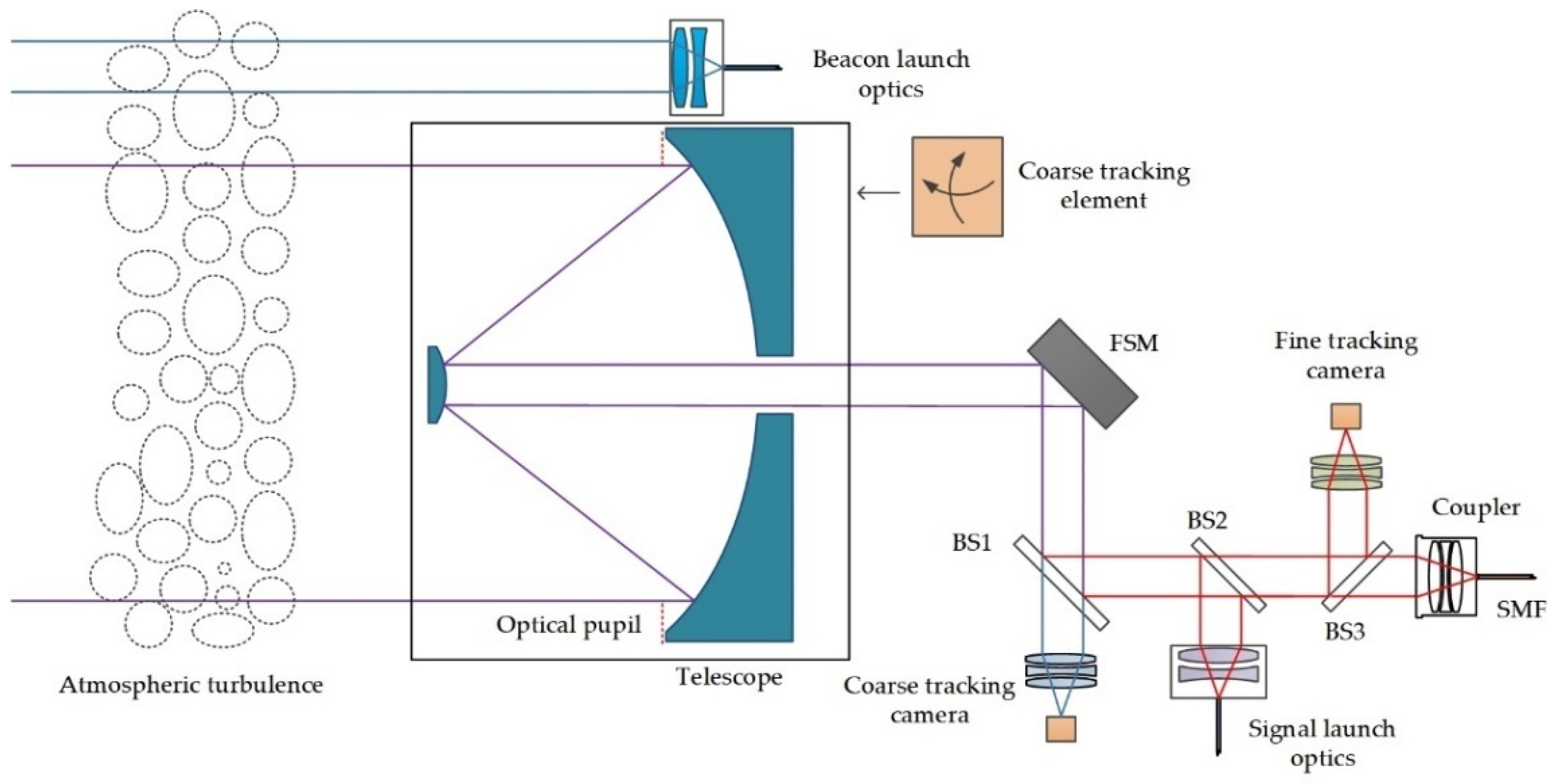
:1. Introduction
2. Theoretical Analysis
- (1)
- The speckles are independent of each other.
- (2)
- The phase distribution function is a Gaussian function related to .
3. Simulation Analysis
| Algorithm 1: The pseudo-code of the simulation progress |
| Input: System parameters and turbulence conditions (). Output: Distribution of CE |
| 1: Choose variable parameter (or ) |
| 2: Initialize (or ) with solid value. |
| 3: Initialize (or ) with the range chosen properly |
| 4: for episode = 1, 2… do as follows |
| 5: Calculate the intermediate variable , , , and |
| 6: Calculate the intermediate variable c and |
| 7: Analyze the PDF based the results of step 6 |
| 8: end for |
| 9: Analyze the distribution of CE |
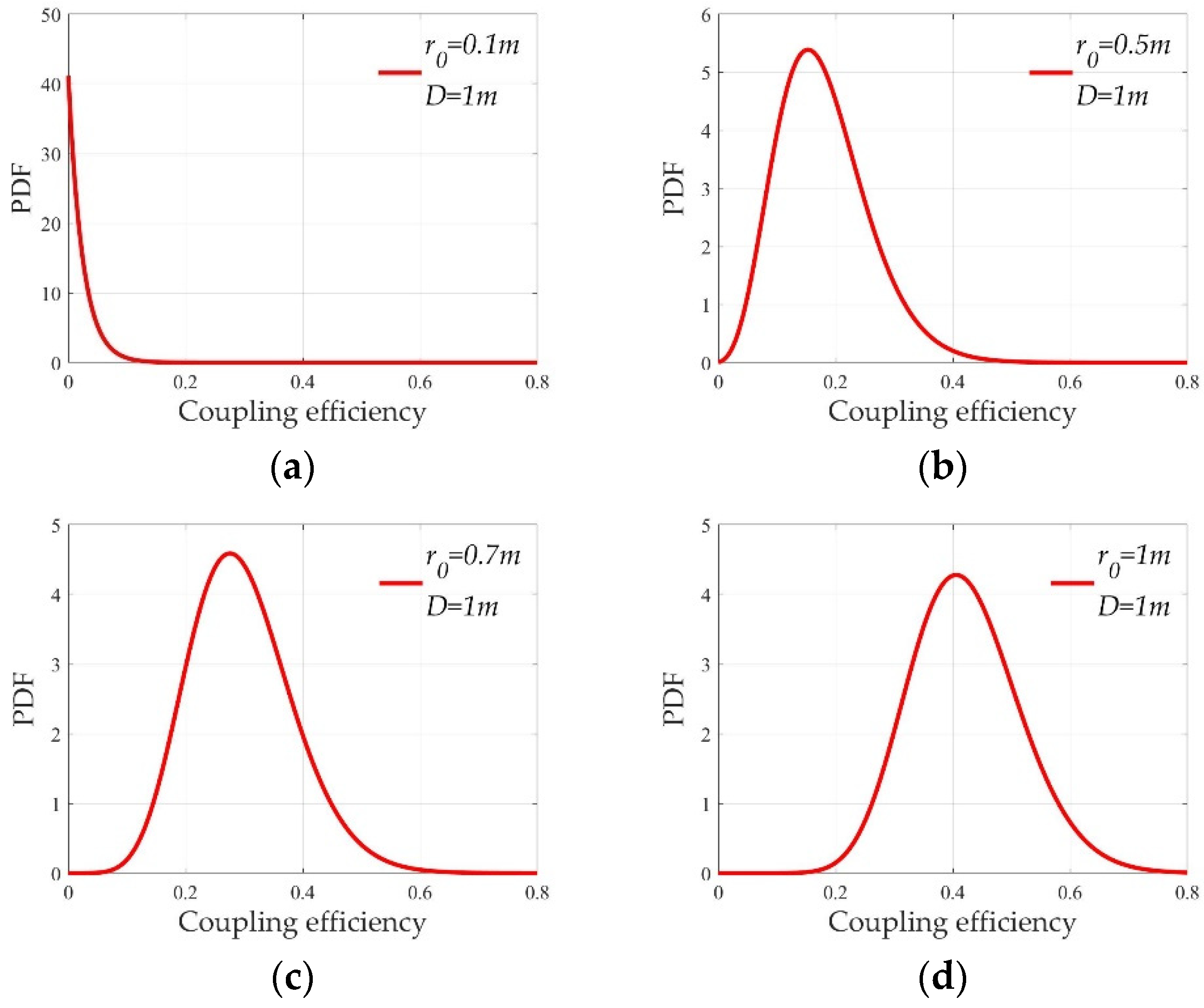
3.1. Solid with Variable
3.2. Solid with Variable
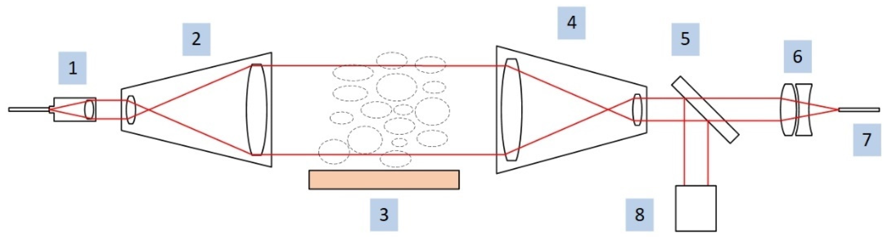
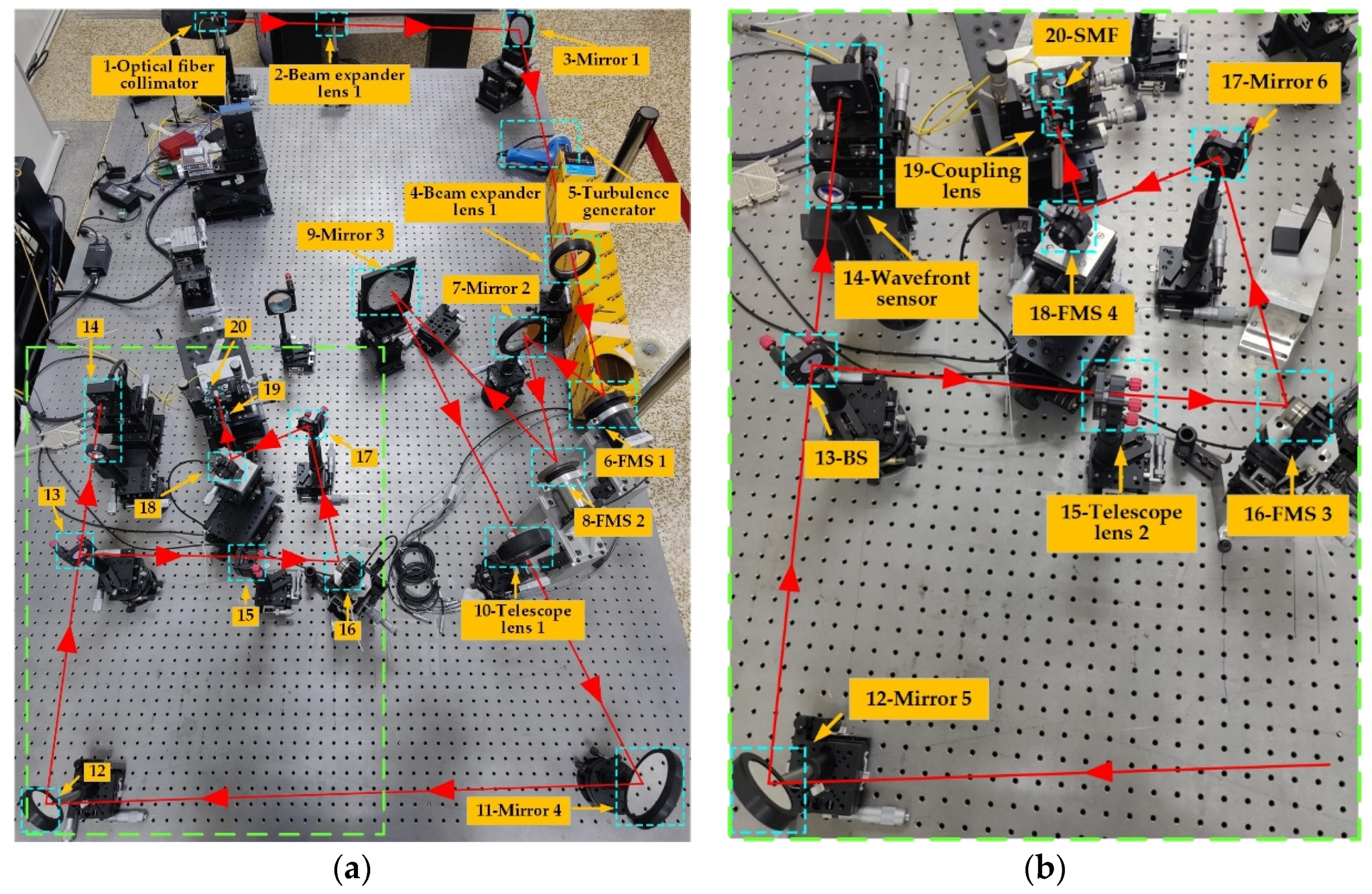
4. Experimental Verification
4.1. Experimental Instruments
4.2. Results and Discussion
5. Conclusions
Author Contributions
Funding
Institutional Review Board Statement
Informed Consent Statement
Conflicts of Interest
Appendix A. Calculation of
References
- Hauschildt, H.; Elia, C. Esas scylight programme: Activities and status of the high throughput optical network “hydron”. Proc. SPIE 2018, 11180, 111800G-1–111800G-8. [Google Scholar]
- Toyoshima, M. Recent trends in space laser communications for small satellites and constellations. J. Lightwave Technol. 2021, 39, 693–699. [Google Scholar] [CrossRef]
- Saathof, R. Optical satellite communication space terminal technology at tno. Proc. SPIE 2018, 11180, 111800K-1–111800K-10. [Google Scholar]
- Andrews, L.C.; Phillips, R.L. Laser Beam Propagation through Random Media, 2nd ed.; SPIE: Bellingham, WA, USA, 2005; pp. 57–60. [Google Scholar]
- Dikmelik, Y.; Davidson, F.M. Fiber-coupling efficiency for free-space optical communication through atmospheric turbulence. Appl. Opt. 2005, 44, 4946–4952. [Google Scholar] [CrossRef]
- Du, W.; Yuan, Q. Scintillation index of a spherical wave propagating through Kolmogorov and non-Kolmogorov turbulence along laser-satellite communication uplink at large zenith angles. J. Russ. Laser Res. 2021, 42, 198–209. [Google Scholar] [CrossRef]
- Be1en’kii, M.S.; Karis, S.J.; Brown, J.M.; Fugate, R.Q. Experimental evidence of the effects of non-Kolmogorov turbulence and anisotropy of turbulence. Proc. SPIE 1999, 3749, 50–51. [Google Scholar]
- Wang, G. A new random-phase-screen time series simulation algorithm for dynamically atmospheric turbulence wave-front generator. Proc. SPIE 2006, 6027, 602716. [Google Scholar]
- Wu, X.; Huang, Y.; Mei, H.; Shao, S.; Huang, H.; Qian, X.; Cui, C. Measurement of non-Kolmogorov turbulence characteristic parameter in atmospheric surface layer. Acta Opt. Sin. 2014, 34, 0601001. [Google Scholar]
- Cui, L.Y.; Xue, B.D. Influence of moderate-to-strong non-Kolmogorov turbulence on the imaging system by atmospheric turbulence MTF. Optik 2015, 126, 191–198. [Google Scholar] [CrossRef]
- Baykal, Y. Coherence length in non-Kolmogorov satellite links. Opt. Commun. 2013, 308, 105–108. [Google Scholar] [CrossRef]
- Yao, J.R. Oceanic non-Kolmogorov optical turbulence and spherical wave propagation. Opt. Express 2021, 29, 1340–1359. [Google Scholar] [CrossRef] [PubMed]
- El-Nahal, F.I. Coherent quadrature phase shift keying optical communication systems. Optoelectron. Lett. 2018, 14, 0372–0375. [Google Scholar] [CrossRef]
- Hu, B.; Zhang, Y. New model of the fiber coupling efficiency of a partially coherent Gaussian beam in an ocean to fiber link. Opt. Express 2018, 26, 25111–25119. [Google Scholar] [CrossRef]
- Chen, X.; Hu, X. High coupling efficiency technology of large core hollow-core fiber with single mode fiber. Opt. Express 2019, 27, 33135–33142. [Google Scholar] [CrossRef] [PubMed]
- Liu, N.; Zhang, J.; Zhu, Z. Efficient coupling between an integrated photonic waveguide and an optical fiber. Opt. Express 2021, 29, 27396–27403. [Google Scholar] [CrossRef] [PubMed]
- Chahine, Y.K.; Wroblewski, A.C. Laser beam propagation simulations of long-path scintillation and fade with comparison to ground-to-aircraft optical link measurements. Opt. Eng. 2021, 60, 036112-1–036112-15. [Google Scholar] [CrossRef]
- Farid, A.A. Outage capacity optimization for free-space optical links with pointing errors. J. Lightwave Technol. 2007, 25, 1702–1710. [Google Scholar] [CrossRef] [Green Version]
- Zhai, C.; Tan, L. Fiber coupling efficiency for a Gaussian-beam wave propagating through non-Kolmogorov turbulence. Opt. Express 2015, 23, 15242–15255. [Google Scholar] [CrossRef]
- Zhai, C.; Tan, L. Fiber coupling efficiency in non-Kolmogorov satellite links. Opt. Commun. 2015, 336, 93–97. [Google Scholar] [CrossRef]
- Hua, B.; Xu, Y. Coupling efficiency of a partially coherent laser beam from the anisotropy and non-Kolmogorov marine-atmosphere turbulence to fiber. Optik 2019, 183, 1–6. [Google Scholar] [CrossRef]
- Zhao, X.; Jiang, H.; Han, C. Fiber coupling efficiency on focal plane spot extension caused by turbulence. Optik 2013, 124, 1113–1115. [Google Scholar] [CrossRef]
- Wang, C.; Jiang, L. Fiber-coupling efficiency for a Gaussian-beam wave passing through weak fluctuation regimes. J. Laser Appl. 2017, 29, 032001-1–032001-7. [Google Scholar] [CrossRef]
- Chen, M.; Liu, C. Experimental demonstration of single-mode fiber coupling over relatively strong turbulence with adaptive optics. Appl. Opt. 2015, 54, 8722–8726. [Google Scholar] [CrossRef] [PubMed]
- Bian, Y.; Li, Y. Free-space to single-mode fiber coupling efficiency with optical system aberration and fiber positioning error under atmospheric turbulence. J. Opt. 2022, 24, 025703. [Google Scholar] [CrossRef]
- Li, Y.; Zhu, W. Equivalent refractive-index structure constant of non-Kolmogorov turbulence. Opt. Express 2015, 23, 23004–23012. [Google Scholar] [CrossRef]
- Zeng, A.P.; Huang, Y.P. Spreading of partially coherent polychromatic Hermite-Gaussian beams propagating through non-Kolmogorov turbulence. Opt. Commun. 2012, 285, 4825–4830. [Google Scholar] [CrossRef]
- Robert, J. Noll Zernike polynomials and atmospheric turbulence. J. Opt. Soc. Am. 1976, 66, 207–211. [Google Scholar]
- Boreman, G.D.; Dainty, C. Zernike expansions for non-Kolmogorov turbulence. J. Opt. Soc. Am. A 1996, 13, 517–522. [Google Scholar] [CrossRef]
- Cagigal, M.P.; Canales, V.F. Speckle statistics in partially corrected wave fronts. Opt. Lett. 1998, 23, 1072–1074. [Google Scholar] [CrossRef]
- Jing, M.; Lie, M. Statistical model of the efficiency for spatial light coupling into a single-mode fiber in the presence of atmospheric turbulence. Appl. Opt. 2015, 54, 9287–9293. [Google Scholar]
- Jing, M.; Fang, Z. Plane wave coupling into single-mode fiber in the presence of random angular jitter. Appl. Opt. 2009, 48, 5184–5189. [Google Scholar]


| Ref. | [19] | [20] | [21] | [22] | [23] | [24] | [25] | |
|---|---|---|---|---|---|---|---|---|
| Study type | Theory | √ | √ | √ | √ | √ | √ | √ |
| Simulation | √ | √ | √ | √ | √ | √ | √ | |
| Experiment | - | - | - | - | - | √ | - | |
| Turbulence model | Kolmogorov | - | - | - | √ | √ | √ | √ |
| Non-Kolmogorov | √ | √ | √ | - | - | - | - | |
| Result form | Analytical expression | - | - | - | - | - | - | - |
| Complex integral | √ | √ | √ | √ | √ | √ | √ | |
| Statistical distribution of CE | - | - | - | - | - | - | - | |
| m | 0 | 1 | 2 | 3 | |
|---|---|---|---|---|---|
| n | |||||
| 0 | |||||
| 1 | |||||
| 2 | |||||
| 3 | |||||
| Items | Value |
|---|---|
| Wavelength (λ) | 1550 nm |
| Pupil aperture (D) | 1 m |
| Focal length of coupling system (F) | 4.17 m |
| MFD of single-mode fiber (d) | 5.5 μm |
| 0.1~1 m | |
| β | 11/3 |
| Items | Value |
|---|---|
| Wavelength (λ) | 1550 nm |
| Pupil aperture (D) | 1 m |
| Focal length of coupling system (F) | 4.17 m |
| MFD of single-mode fiber (d) | 5.5 μm |
| ) | 0.5 m |
| β | 2.35~3.76 |
| Items | Value |
|---|---|
| Wavelength | 1550 ± 0.5 nm |
| Divergence angle of the fiber collimator | 1.2 mrad |
| Magnification of beam expander system (2 and 4) | 10× |
| Diameter of coupling lens | 12.7 mm |
| Focal length of coupling lens | 53 mm |
| Magnification of the receiving telescope (10 and 15) | 1/3× |
| Single-mode fiber | Corning SMF-28e |
| r0 (m) | Non-Kolmogorov Model | Kolmogorov Model Correlation Coefficients | |
|---|---|---|---|
| β | Correlation Coefficients | ||
| 0.134 | 2.79 | 0.9765 | 0.6546 |
| 0.105 | 2.89 | 0.9537 | 0.8378 |
| 0.035 | 3.78 | 0.9783 | 0.9213 |
| 0.023 | 3.95 | 0.9898 | 0.9762 |
| 0.016 | 3.61 | 0.9945 | 0.9908 |
Publisher’s Note: MDPI stays neutral with regard to jurisdictional claims in published maps and institutional affiliations. |
© 2022 by the authors. Licensee MDPI, Basel, Switzerland. This article is an open access article distributed under the terms and conditions of the Creative Commons Attribution (CC BY) license (https://creativecommons.org/licenses/by/4.0/).
Share and Cite
Ma, L.; Gao, S.; Chen, B.; Liu, Y. Theoretical and Experimental Analysis on Statistical Properties of Coupling Efficiency for Single-Mode Fiber in Free-Space Optical Communication Link Based on Non-Kolmogorov Turbulence. Appl. Sci. 2022, 12, 6075. https://doi.org/10.3390/app12126075
Ma L, Gao S, Chen B, Liu Y. Theoretical and Experimental Analysis on Statistical Properties of Coupling Efficiency for Single-Mode Fiber in Free-Space Optical Communication Link Based on Non-Kolmogorov Turbulence. Applied Sciences. 2022; 12(12):6075. https://doi.org/10.3390/app12126075
Chicago/Turabian StyleMa, Lie, Shijie Gao, Bo Chen, and Yongkai Liu. 2022. "Theoretical and Experimental Analysis on Statistical Properties of Coupling Efficiency for Single-Mode Fiber in Free-Space Optical Communication Link Based on Non-Kolmogorov Turbulence" Applied Sciences 12, no. 12: 6075. https://doi.org/10.3390/app12126075
APA StyleMa, L., Gao, S., Chen, B., & Liu, Y. (2022). Theoretical and Experimental Analysis on Statistical Properties of Coupling Efficiency for Single-Mode Fiber in Free-Space Optical Communication Link Based on Non-Kolmogorov Turbulence. Applied Sciences, 12(12), 6075. https://doi.org/10.3390/app12126075