Single Image Super-Resolution Method Based on an Improved Adversarial Generation Network

Abstract

Super-Resolution (SR) techniques for image restoration have recently been gaining attention due to their excellent performance. For powerful learning abilities, Generative Adversarial Networks (GANs) have been proven to have achieved great success. In this paper, we propose an Enhanced Generative Adversarial Network (EGAN) for improving its effects for a real-time Super-Resolution task. The main content of this paper are as follows: (1) We adopted the Laplacian pyramid framework as a pre-trained module, which is beneficial for providing multiscale features for our input. (2) At each feature block, a convolutional skip-connections network, which may contain some latent information, was significant for the generative model to reconstruct a plausible-looking image. (3) Considering that the edge details usually play an important role in image generation, a perceptual loss function was defined to train and seek the optimal parameters. Quantitative and qualitative evaluations were demonstrated so that our algorithm not only took full advantage of the Convolutional Neural Networks (CNNs) to improve the image quality, but also performed better than other algorithms in speed and performance for real-time Super-Resolution tasks.

1. Introduction

Super-Resolution (SR) has become a hot topic in the computer vision research community, since it reconstructs a high-resolution (HR) image from the low-resolution (LR) information provided. SR has a wide range of applications in medical imaging, and in security and surveillance, where high-frequency details are required on demand [1]. The dilemma of SR is that it is an ill-posed inverse problem, since multiple HR patches are consistent with the given LR patch. To address this issue, additional prior knowledge has to be made regarding the formation of the desired HR images.

Recently, deep-learning methods have exhibited excellent performance in SR tasks. The data-driven method has also been used with large improvements in accuracy; this includes convolutional neural network (CNN)-based methods [2]. For example, the pioneer CNN model for SR has gained considerable attention because of its portable architecture. This method [3], termed Super-Resolution Convolutional Neural Network (SRCNN), provides compelling quality and outperforms traditional non-deep-learning algorithms. Subsequently, many follow-up methods have shown their advantages for SR tasks. Kim et al. [4] deployed gradient clipping and residuals-learning to predict the residuals instead of actual pixels. Lai et al. [5] proposed the Deep Laplacian Pyramid Network (LapSRN) by upscaling from a small to a large upscaling factor. They progressively predicted the sub-band residuals ranging from coarse to fine levels. With the further development of CNNs, they deployed some skip-connections to improve the image quality. The Deep Recursive Residual Network (DRRN) jointly utilizes skip-connections to fully exploit the latent information [6]. At present, the real-time performances of existing networks are poor, the sample data are difficult to obtain, and the restoration effect is not ideal.

To date, convolutional neural networks have become increasingly powerful in computer vision applications. However, there has been less attention paid to CNNs that discriminate whether the extracted features are robust, based on their potential to train high-dimensional, complex real data [7]. There are two outstanding algorithms, Variational AutoEncoders (VAE) and Generative Adversarial Networks (GANs), that have excellent performances compared with state-of-the-art algorithms for image processing. The VAE [8] is an attractive model, since it learns complex probability distributions from training data. However, the high-quality images significantly depend on the expressiveness of the inference model. In other words, the VAE is not expressive enough when it is trained on true posterior distributions. The GANs [9] mimic the target distribution through the construction of a generative model. The networks represent two parts of the generator and discriminator to extract features for SR tasks. The algorithm of the GAN may be characterized as a two-player minimax game between the generative model, which tries to produce counterfeit data without detection, and the discriminative model, which learns to distinguish between the synthesized images from the generator and the real images from data distribution. On the one hand, a noise variable z can be defined as the generative model input. Goodfellow et al. then incorporated the noise z into the model G to generate the synthesized images G(z). Furthermore, the parameters of network G can be optimized constantly based on the feedback information given by the discriminator. On the other hand, the discriminative model D can be viewed as mappings from the data distribution: $D\left(x\right)\underset{\mathrm{dicriminator}}{⟶}(0,1)$. It determines whether the images are from the generator (false, close to 0) or from the data distribution (true, close to 1). For the discriminative model D, training the parameters of D via fixing the generator can classify images. Specifically, they achieve this strategy with the utility of two joint adversarial networks. This achieves a balance when the synthesized images G(z) are similar to real images from the data distribution, and the discriminator D predicts 0.5 between G(z) and the real images for most inputs. Both the networks of G and D have learned the capacity sufficiently, which is called the Nash equilibrium [10]. Unfortunately, some of the GAN structures are unstable during the training performance, which causes that lead generator to produce some artifacts and nonsensical outputs. Considering that the CNN architecture has a remarkable performance in terms of feature extraction, we take advantage of CNNs to construct our generator, and then utilize a discriminator to test whether the generated images satisfy the SR performance.

Quantitative and qualitative evaluations have been demonstrated so that our algorithm not only takes full advantage of the Convolutional Neural Networks (CNNs) to improve the image quality, but it also performs better than previous GAN algorithms for super-resolution tasks.

Super-resolution reconstruction is very important for acquiring image information and reconnaissance detection. Existing works have some problems, such as a weak generalization ability and a large space for the mapping function solution. Our framework improves the resolution detail of the image texture, which provides original materials for subsequent image processing.

In this paper, we propose Enhanced Generative Adversarial Networks (EGAN) in order to efficiently correct these issues. The main contributions of our network are as follows:

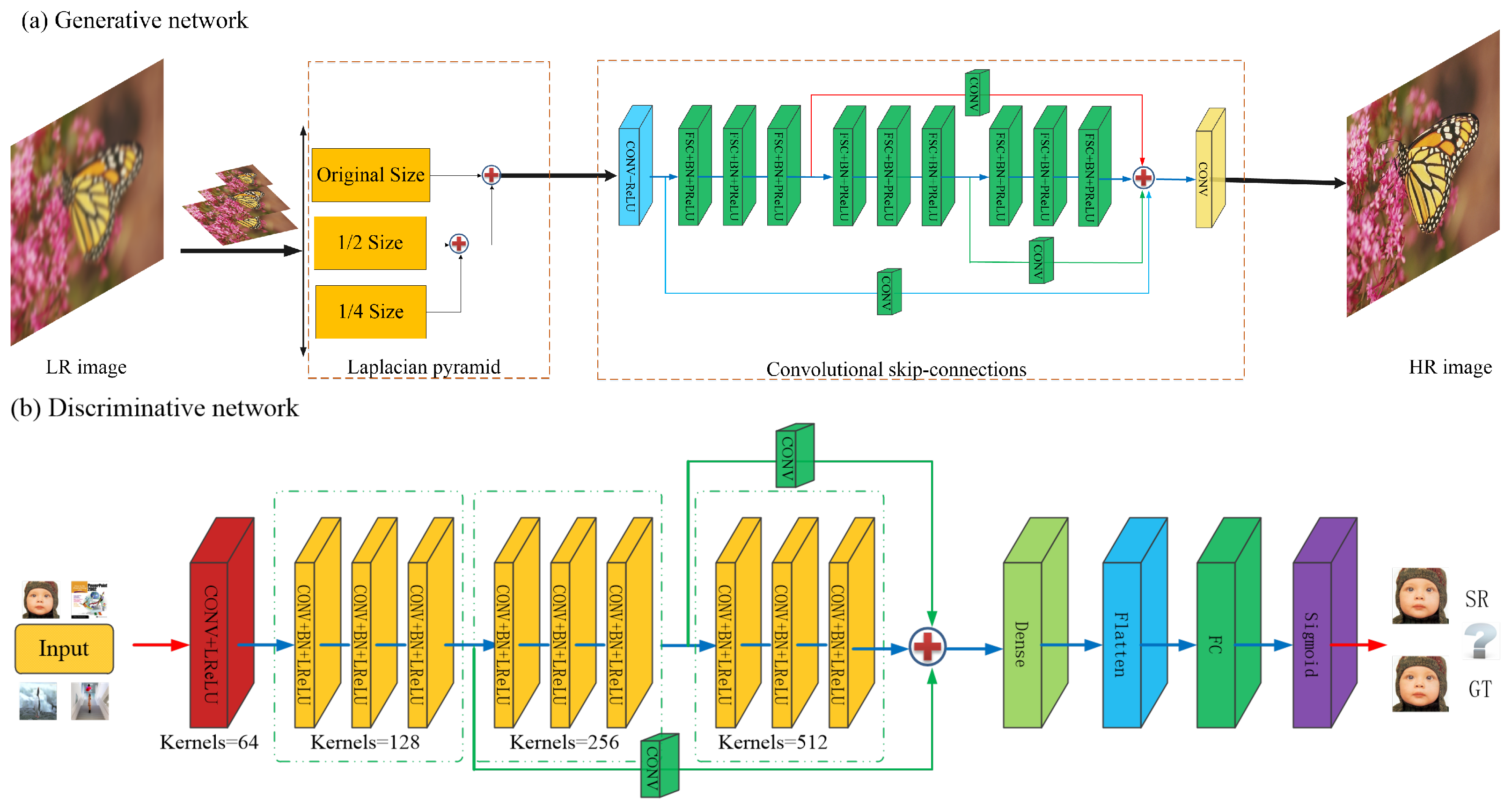
• Convolutional skip-connections: Some CNN algorithms show significant advantages for SR tasks. Different from cascade networks in typical methods, we design a convolutional skip-connections network based on an end-to-end manner. Note that feature maps from the intermediate layers may contain some latent information. It is crucial for the generative model to generate a plausible-looking image that relies on the convolutional skip-connections. Therefore, our generator can project some high-frequency details onto the synthesized images to fool the discriminator, D.
• Perceptual loss function: Normally, several GAN methods are limited by instability learning during training. We propose a perceptual loss function to penalize the samples in our adversarial network. Considering that the edge details usually play a significant role in image generation, the generator produces synthesized images that are closer to the real images via our loss function. Moreover, our loss function corrects the errors between the real images and the generated images, which improves the accuracy of the discriminator.

2. Related Work

In this section, we discuss some typical SR algorithms, i.e., deep-learning. This includes both CNN-based methods and GAN-based algorithms. Meanwhile, a brief introduction to SR techniques and some typical GAN algorithms are illustrated. The detailed information for SR will be discussed in the following sections.

2.1. Typical Image SR Algorithms

In generally, there are three categories for SR techniques. Earlier interpolation methods, such as bicubic interpolation and Lanczos resampling [11] can predict the center pixel using neighboring pixels. Although these interpolation methods are very fast, the edge information cannot be recovered effectively. To avoid edge artifacts, learning-based approaches [12,13,14] can improve the resolution with the help of prior knowledge. However, the prediction relies significantly on prior knowledge. This makes the effect in reconstruction drop dramatically while processing complex images. Due to its powerful learning ability, the deep-learning [15,16,17,18,19] algorithms have shown greater degrees of performance than the traditional methods in SR tasks. As the pioneer CNN model for SR, there are three convolutional blocks in SRCNN: feature extraction, non-linear mapping, and reconstruction. They learn implicit mapping through the CNN model and use this mapping to recover the HR image from an interpolated image. Unfortunately, considering the limitations of the network layers, there is some characteristic information that is not well introduced for the further improvement of image quality. Under its powerful calculating capabilities, an increasing number of CNN-based methods have attracted attention in SR tasks. These include Fast Super Resolution Convolutional Neural Networks (FSRCNN), Very Deep Convolutional Network (VDSR), Deeply Recursive Convolutional Network (DRCN), and Deep Recursive Residual Network (DRRN). Meanwhile, Goodfellow et al. [9] proposed a GAN that has become more popular and well-known in the deep-learning field. Various kinds of GANs have been proposed in recent years. Under the guidance of network structure, the Laplacian Pyramid of Generative Adversarial Network (LapGAN) produces sharp images using the Laplacian pyramid [20]. The Deep Convolutional Generative Adversarial Network (DCGAN) has demonstrated great feature representations using fully convolutional networks in the generator [21], instead of deterministic spatial pooling functions. Even more excellent and effective are the perceptual loss functions, including a content loss and an adversarial loss in Super-Resolution using a Generative Adversarial Network (SRGAN) [22], which achieves state-of-the-art performance. In addition, other deep-learning algorithms also achieve good results, such as the DRCN [23], InfoGAN [24], CGAN [25], and CycleGAN [26].

2.2. SR Based on Deep-Learning Algorithms

Recently, SR based on deep-learning algorithms have been proven to achieve great success. Many learning models have attracted increasing attention due to their powerful capabilities. To enrich the image details, a multiscale dictionary is presented by Zhang et al. [27]. The related methods for SR tasks originate in compressed sensing [28,29]. Under the mapping between the LR and HR images, Simonyan and Zisserman propose a deeper network architecture to increase the accuracy, relying on a high degree of complexity [30]. In Denton et al., the authors present a generative model with a Laplacian pyramid network (LAPGAN) that is similar to our pre-trained module. The RefineNet [15] fuses finer-grained features with semantic information through a multipath architecture, which generates semantic HR images, as given by Lin et al. This method also facilitates gradient propagation during end-to-end training. The skip-connections [23,31] as an effective design are used to tackle the gradient vanishing problem. Meanwhile, it is beneficial for skip-connections to carry significant information during the forward propagation. For these reasons, the DRRN adopts many skip-connections between the convolutional layers to improve the SR performance. In addition, Salimans [32] et al. present feature matching to accelerate convergence using the mean squared error (MSE). This assists the discriminator in handling some images that are poor in high-frequency details. In Ledig et al. [18], the authors use a perceptual loss function based on the VGG19 network to generate more photo-realistic images than typical algorithms. According to related work, an enhanced architecture is crucial for the GAN algorithm.

3. An Enhanced Generative Adversarial Network for SR

In this section, we begin to describe our network for SR tasks. As shown in Figure 1, the structure of our algorithm mainly consists of two networks, including the generative network structure and the adversarial network structure. According to the typical SR approach using GAN methods, our generative network can be divided into three modules. On the one hand, inspired by the LapGAN [20], we employ an improved input using the Laplacian pyramid as our pre-trained module to refine image features. Since the feature maps of convolutional extraction may be “influenced” by the next layer, we add some convolutional skip-connections to obtain more latent information. Additionally, the loss function is perceptual for our generative network to optimize its parameters. On the other hand, we improve the discriminative network summarized by Ledig et al. [18] to design our structure.

Our discriminative network is constantly trained to distinguish the synthesized images from the generator, and the real images from the data distribution.

3.1. Generative Network Structure

3.1.1. Laplacian Pyramid

Recently, the Laplacian pyramid framework has shown a powerful capability using a coarse-to-fine model as Figure 2 shown. Considering the remarkable performance, we adapt this framework as our pre-trained module. In our network, the generator takes a noise variable z as its input and produces an image, I. Normally, down(•) denotes a down-sample operator to blur and extract an s×s image, I, and down(I) becomes a new size, s/2 × s/2. Meanwhile, up(•) represents an up-sample operation to double the size of the image, so that up(I) turns into a larger image (2 s × 2 s).

Resampling can be used to keep specific information (so that target information is not lost) and to consciously change the distribution of the samples to suit the training and learning of subsequent models.

• We construct a Gaussian pyramid G(I) = [$I_1$, $I_2$, …, $I_N$]; here, $I_1$ = I and $I_N$ is N recursive applications of down(•) to I. The $I_N$ can be viewed as the Nth number of levels in the pyramid. In addition, the top level has to retain a certain size because the image has too few pixels to recover (we usually set N = 3 in the pre-trained module). We initialize the down-top levels with the Gaussian kernel w, and then remove the even lines:

  $$I_N(i,j)=\sum _{m=-2}^2\sum _{n=-2}^{2}w(m,n)·I_{N-1}(2i+m,2j+n)$$

  (1)
• The image $L_N$(I) denotes the Nth levels of the Laplacian pyramid, which is made up of two adjacent levels in the Gaussian pyramid. Then, we up-sample the smaller image with the up(•) operator, so that the image $L_N$(I) sizes can be expressed as:

  $$L_N\left(I\right)=G_N\left(I\right)-up\left(G_{N+1}\left(I\right)\right)=I_N-up\left(I_{N+1}\right)$$

  (2)

Obviously, each level corresponds to a scale image. As a low-frequency residual, the top-level image can be equal to the Gaussian pyramid, such as $G_N$(I) = $L_N$(I). The finest image in the pre-trained module is calculated by combining the Laplacian pyramid image with the backward recurrence, and the resultant $I_N$ can also be viewed as:

$$I_N=up\left(I_{N+1}\right)+L_N\left(I\right)$$

(3)

The initial image is $I_N=L_N\left(I\right)$, and the finest image is $I_1=I_N$. In summary, beginning with the coarsest level, we alternately up-sample and add a particular scale image, $L_N\left(I\right)$, from the following finer level. Finally, we can calculate the finest image in the pre-trained module.

3.1.2. Convolutional Skip-Connections

The typical CNN algorithms have been proven to exhibit great advantages for SR tasks [33]. These CNN-based algorithms extract effective and robust features from LR information using convolutional layers such as SRCNN, VDSR, and DRRN. The convolution and ReLU operator can be viewed as:

$$f\left(x\right)=max(w\otimes x+b,0)$$

(4)

However, some GAN methods are not successfully applied to image super-resolution. The authors of DCGAN utilize a cascade convolutional network to generate image representations. Although the above algorithm extracts the image features using a convolutional neural network, the cascade architecture limits the generator to learn deep semantic features. We argue that feature maps from the intermediate layers may contain some latent information that are crucial for image representations. Therefore, it is important for our generator to employ some convolutional skip-connections and then to extract feature maps from the intermediate layers, which effectively avoids deep semantic loss. The deployed convolutional skip-convolutions can be represented by the following in Figure 3.

The convolutional skip-connections play a significant role in both the forward propagation and the backward propagation. On the one hand, each convolutional skip-connection introduces a convolutional layer that is compared with traditional skip-connections, which slightly adjusts the feature maps that are extracted during the forward propagation. On the other hand, our convolutional skip-connections alleviate the gradient vanishing problem in the backward propagation, because the gradient is passed directly by our convolutional skip-connections.

Specifically, we use small 3 × 3 kernels for the convolutional layers, as inspired by Gross et al. [31], and we use the activation function ReLU as our first block. From the second to fourth blocks, a series of fractional-strided convolutions (FSC) are applied to all convolutional layers, as proposed by Radford. Considering that batch normalization (BN) is usually utilized to counteract the internal covariate shift [34], the BN helps to bridge between the fractional-strided convolutions and ParametricReLU. For the activation function PReLU, the mathematical formulation can be expressed as:

$$PReLU=max(x,0)+amax(0,x)$$

(5)

where x denotes the input signal, and the parameter a is learnable for the PReLU in the negative portion, which effectively alleviates the “dead feature” in the zero gradients [35]. In the fifth block, the convolutional layer generates a plausible-looking image, with the goal of fooling the discriminative model D.

3.2. Discriminative Network Structure

The discriminator constantly improves the learning ability to distinguish between generated images and real images during the training procedure. As shown in Figure 1, our discriminative network is optimized in structure compared with the traditional discriminator.

Specifically, we employ 10 convolutional layers sized at 3 × 3 kernels. To obtain more context, the size of the receptive field is increased by a factor of 2, from 64 to 512. Considering that the sizes are proportional to the layers, we follow the available framework of the VGG19 network. Similar to the generator, there are three CBL modules in our discriminative network. Each CBL module contains the convolutional layers BN and LReLU. We also employ two convolutional skip-connections after each CBL module, which can obtain more high-frequency details to distinguish the images. The convolutional layers are used to extract abundant features. The 512 results are followed by a dense layer and a flattened layer. These operations map each multidimensional input onto another one-dimensional vector. Then, the vectors are fed into fully connected layers to combine the features from the previous layers. Finally, a sigmoid function with one node produces a probability for the classification.

3.3. Perceptual Loss Function

A two-player minimax game proposed by Goodfellow et al. [9] has been proven to show a relatively good performance for loss functions. Firstly, the authors incorporate noise z from the distribution in the generative model G over data x as an input variable $p_z\left(z\right)$. Secondly, they map the input z to the data space $G(z;\theta )$ over the generative network. During the training procedure, the generator has enough capacity to fool the discriminative model in order to maximize the probability that the discriminator believes the fake samples from the real images. The generative model G is trained to minimize the $log(1-D(G\left(z\right)\left)\right)$. Thirdly, the discriminative model D constantly improves its learning ability, and then it distinguishes whether the images are from the generator or from the data distribution. Likewise, they maximize the $log\left(D\right(x\left)\right)$ for the discriminator. The value function for the GAN is composed as follows:

$$\underset{G}{min}\underset{D}{max}V(D,G)=E_{x\sim p_{\mathrm{data}}\left(x\right)}[logD\left(x\right)]+E_{z\sim p_z\left(z\right)}[log(1-D\left(G\left(z\right)\right))]$$

(6)

When G and D have been sufficiently trained, they will reach a stationary point where they both converge to a Nash equilibrium. Then, the discriminative model D can be denoted in Equation (7) via a fixed G.

$$D_G^{\#}\left(x\right)=\frac{p_{\mathrm{data}}\left(x\right)}{p_{\mathrm{deta}}\left(x\right)+p_g\left(x\right)}$$

(7)

When reaching a stationary Nash equilibrium for $p_g$ = $p_{data}$, we use $D_G^{\#}\left(x\right)$ to denote $D_{\left(x\right)}$ for simplicity, and Equation (8) can be reformulated as:

$$\begin{array}{cc}\hfill \underset{D}{max}V\left(D^{\#},G\right)& =E_{x\sim p_{\mathrm{data}}}\left[log{D}_G^{\#}\left(x\right)\right]+E_{z\sim p_z}\left[log\left(1-D_G^{\#}\left(G\left(z\right)\right)\right)\right]\hfill \end{array}$$

(8)

$$\begin{array}{cc}& =E_{x\sim p_{\mathrm{data}}}\left[log\frac{p_{\mathrm{data}}\left(x\right)}{p_{\mathrm{data}}\left(x\right)+p_g\left(x\right)}\right]+E_{z\sim p_z}\left[log\frac{p_g\left(x\right)}{p_{\mathrm{data}}\left(x\right)+p_g\left(x\right)}\right]\hfill \end{array}$$

(9)

$$\begin{array}{cc}& ={\int }_x{p}_{\mathrm{data}}\left(x\right)log\frac{\frac{0.5\times p_{\mathrm{data}}\left(x\right)}{p_{\mathrm{data}}\left(x\right)+p_g\left(x\right)}}{2}dx+{\int }_x{p}_g\left(x\right)log\frac{\frac{0.5\times p_g\left(x\right)}{p_{\mathrm{data}}\left(x\right)+p_g\left(x\right)}}{2}dx\hfill \end{array}$$

(10)

$$\begin{array}{cc}& =2log\frac{1}{2}+{\int }_x{p}_{\mathrm{data}}\left(x\right)log\frac{\frac{p_{\mathrm{data}}\left(x\right)}{p_{\mathrm{data}}\left(x\right)+p_g\left(x\right)}}{2}dx+{\int }_x{p}_g\left(x\right)log\frac{\frac{p_g\left(x\right)}{p_{\mathrm{data}}\left(x\right)+p_g\left(x\right)}}{2}dx\hfill \end{array}$$

(11)

$$\begin{array}{cc}& =2log\frac{1}{2}+2JSD\left(p_{\mathrm{data}}\left(x\right)\parallel p_g\left(x\right)\right)\hfill \end{array}$$

(12)

Here, the JSD(x||y) function is the abbreviation of the Jensen–Shannon Divergence between the generative model and the data distribution [26]. However, the above loss function exhibits some limitations. For instance, the discriminator only focuses on whether the input is effectively distinguished (true or false), but there is no penalty for D when it misclassifies those fake samples. This easily causes the gradient vanishing problem where a saddle point may be found. Inspired by LSGAN, Mao et al. [30] adopted the least squares loss function for the discriminative model. Based on this observation, we employed an energy-based regularization term as part of our loss function, to further improve the accuracy of the GAN. Since the center pixels in the synthesized images were correlated with their neighboring ones, we argued that the generator could autonomously converge to reach a point where there is lower energy and it is more stable, under the conditions of a regularization term.

In our adversarial network, the generator and discriminator have different perceptional loss functions, respectively. There are three parts for the generative loss function, which includes content loss, adversarial loss, and energy-based regularization. We define the content loss as the MSE between the synthesized images $G\left(z\right)$ from the generator and the real images x, from the data distribution. The content loss ensures the $G\left(z\right)$ and x are closer to perceptual similarity during the training. While having enough capacity to fool the discriminative model, this encourages the adversarial loss to minimize the error $\left(D\right(G\left(z\right))-1)$ as little as possible. Although each pixel $x_i$ in the images has more or less correlation with neighbors of $x_j$ in the batch $x_1$, …, $x_n$, there are significant differences between the pixels on the edge. According to [36], we adopt the energy-based regularization $E(z_i,z_j)$ to restrict the relationship between the center pixels and the neighboring ones generated by G. Our generative loss function can be formulated as follows:

$$L_G(x,z)=n_1{\parallel G\left(z\right)-x\parallel }_F^2+n_2{\parallel D\left(G\left(z\right)\right)-1\parallel }_F^2+n_3\sum _{i,j}E\left(z_i,z_j\right)$$

(13)

Here, $\left|\right|•{\left|\right|}_F$ denotes the Frobenius norm, and the coefficients $n_1$ = 1, $n_2$ = 0.1, and $n_3$ = 0.1 in our experiment. The energy-based regularization ${\sum }_{i,j}E\left(z_i,z_j\right)$ for the calculation is as follows:

$$\sum _{i,j}E\left(z_i,z_j\right)=\sum _{i=1}^{16}\sum _{j=1}^{16}G\left(z_i,z_j\right)·exp\left(-\frac{{∥z_i-z_j∥}^2}{2a^2}\right)+\left(1-G\left(z_i,z_j\right)\right)·exp\left(-\frac{{∥1-\mid z_i-z_j∥}^2}{2b^2}\right)$$

(14)

where $z_i$, $z_j$ represents the center pixel and its 16 connected pixels, respectively. $G(z_i,z_j)$ denotes the gradient to reduce the error probability. In the Equation (10), we set a = 1 and b = 1 for simplicity. Note:

$$\left\{\begin{array}{cc}G\left(z_i,z_j\right)=0\hfill & \mathrm{if}{z}_i=z_j\hfill \\ G\left(z_i,z_j\right)=1\hfill & \mathrm{otherwise}\hfill \end{array}\right.$$

(15)

Likewise, the discriminator as a classifier can determine whether the images are from the generator or the data distribution, if given training time. Our discriminative loss function not only calculates the MSE in the case of discriminator misclassification, but it also has enough capacity to distinguish between real images and generated images. Therefore, the discriminative loss function effectively avoids mode collapsing and increases the performance accuracy. Therefore, we have the following loss function:

$$L_D(x,G\left(z\right))=\frac{1}{2}{\parallel D\left(x\right)-1\parallel }^2+\frac{1}{2}{\parallel D\left(G\left(z\right)\right)\parallel }^2$$

(16)

In summary, our perceptual loss function, including the generative and discriminative parts, is significant for our network, since it refines the high-frequency details and corrects the errors between the real images and the generated images.

4. Experiments

In this section, we demonstrate the excellent perceptual performance of our network, and we make visual and quantitive comparisons with several state-of-the-art algorithms. There are three subsections as follows: First, we brief our algorithm; then, we introduce some details in the modified network structure, such as the Laplacian pyramid, convolutional skip-connections, and perceptual loss function; lastly, we compare the performance with several existing algorithms based on public datasets to illustrate the effectiveness of our algorithm.

4.1. Experimental Dataset and Setting

To increase the diversity of the training samples, flipping and rotation techniques are introduced into a large database. For example, we rotate the images by 0°, 90°, 180°, or 270° to generate different directions. Then, we randomly flip between the horizontal or vertical images. Additionally, there are four different scales, including ×0.9, ×0.8, ×0.7, and ×0.6 for the training images to enlarge the multiscale samples. After data augmentation, the dataset made up of 600,000 images from the ImageSet dataset [37] was divided into a validation set and training set, with a ratio of 8:2. For testing, the benchmark datasets, including Set5 [35], Set14 [38], BSD100 [36], and Urban100 [39] are adopted, respectively.

Most of the experiments are performed between the LR and HR images at a scale factor of ×2, ×3, and ×4. For a fair comparison, the averaged peak signal-to-noise ratio (PSNR), the structural similarity index (SSIM), and the information fidelity criterion (IFC) are calculated for quantitative evaluation. In addition, the SR images for the methods, which include SRCNN, VDSR, DRRN, and SRGAN, are obtained from Huang et al., and are available online.

Our network is conducted on a workstation with an Intel i9 12900K CPU, a Linux operating system, and two GeForce RTX3080Ti GPUs.

4.2. Implementation Details

4.2.1. Laplacian Pyramid Performance

Decreasing by a factor of 1/2 from the original size to 1/4 size in the Laplacian pyramid framework, we obtain the LR images by using a down-sample operator on the HR images. A multiscale Gaussian pyramid G(I) = [$I_1$, $I_2$, $I_3$] has been built. As shown in Figure 4, we use a bicubic kernel (3 × 3) with an up-sampling operation to match the size of the upper layer. Specifically, we first up-sample the 1/4 size image by a factor of 2, and then connect it to the 1/2 size image. Then, we up-sample the 1/2 size with a ×2 factor to match the original-sized image. The up-sample operator on the small images (1/4 size, 1/2 size) are from Equation (2). All path inputs that have the same size are fused into the Laplacian pyramid image.

As shown in

Table 1. Comparison with different sized inputs on BSD100 and Urban100.

		Dataset	BSD100	Urban100
	PSNR(dB)
Inputs
Original size			32.30	30.79
Original size + 1/2 size			32.38	30.88
Original size + 1/2 size +1/4 size			32.41	30.93

, we design different multipath inputs as contrast experiments. We utilize the same parameter configuration to test the representative datasets on B100 and Urban100. The quantitative results have shown that the more input paths, the higher the PSNR. The extra size inputs can provide potential information for the Laplacian pyramid image. Therefore, our pre-trained module not only exploits down-top levels of robust information, but it also produces high-frequency samples for the generative model.

4.2.2. Convolutional Skip-Connections Performance

Noting that the feature maps from the intermediate layers may contain some latent information, we compare the results from three different blocks of convolutional skip-connections (CSC), based on Set14. In

Table 2. Comparison with different convolutional skip connections in each input (for the color of CSC module, refer to Figure 3).

	CSC	1st CSC (Red)	2nd CSC (Blue)	3rd CSC (Green)
Inputs
(a)		√
(b)		√	√
(c)		√	√	√

, the red line represents the first convolutional skip-connection in Figure 3. Similarly, the blue line and green line denote the second convolutional skip-connection and the third convolutional skip-connection, respectively. These three convolutional skip-connections construct a parallel module, which can be expressed as:

$$I_{out}=FBP\left(I_{in}\right)+f_R\left(I_{in}\right)+f_B\left(I_{in}\right)+f_G\left(I_{in}\right)$$

(17)

Here, $I_{in}$ and $I_{out}$ denote the input and output image, respectively. The function FBP is made up of FSC, BN, and PReLU, and we use FBP($I_{in}$) to represent a cascade network. For example, the function $f_R$($I^{in}$) denotes the first convolutional skip-connection with a red line, which is similar to $f_B$($I_{in}$) and $f_G$($I_{in}$).

As shown in Figure 5, the image generated by the third CSC has richer details compared with the other two groups. Thus, our parallel module including three CSCs reconstructs the HR images with more semantic information and more refined feature maps.

4.2.3. Perceptual Loss Function Performance

As stated in Section 3.3, the implementation of the perceptual loss function can be trained to alleviate losses through the adversarial network. In our experiment, we evaluate the performance of three loss functions: SRGAN, EGAN without energy-based regularization, and EGAN with energy-based regularization. The results are shown in Figure 6. On one hand, EGAN has a smaller loss compared with SRGAN, which accelerates the convergence speed. On the other hand, the energy-based regularization overcomes overfitting effectively, and gives the generated images more robust details. When the epochs reach 5000, the loss caused by the generator and the discriminator becomes stable. The converging speed of EGAN with energy-based regularization is the fastest, indicating that the network has a better convergence speed. In other words, G obtained the capacity of generating fake images, and D can also provide real-time feedback for G, which is beneficial for tuning hyperparameters.

Although most GAN algorithms have momentum during the training progress, we use Adaptive Moment Estimation (Adam) [40] for all hyperparameters. This method not only stores the average exponential decay in AdaDelta, but also keeps the average exponential decay from the gradient $M\left(t\right)$, which is similar to the momentum method.

$$M^{*}\left(t\right)=\frac{M\left(t\right)}{1-{\beta }_1^t}$$

(18)

$$V^{*}\left(t\right)=\frac{V\left(t\right)}{1-{\beta }_2^t}$$

(19)

Here, $M\left(t\right)$ and $V\left(t\right)$ are the gradients of first-order and second-order moment estimations, respectively. We set the momentum to ${\beta }_1=0.9$ and ${\beta }_2=0.999$. The variables $M^{*}\left(t\right)$ and $V^{*}\left(t\right)$ can be used as unbiased estimation to correct $M\left(t\right)$, $V\left(t\right)$.

4.3. Comparisons with the State-of-the-Art Algorithms

We compare the proposed EGAN with four state-of-the-art SR algorithms: SRCNN, VDSR, DRRN, and SRGAN. Visual examples are shown from Figure 7, Figure 8, Figure 9 and Figure 10, and the quantitative results are provided in

Table 3. The average PSNR (dB) and SR time (s) for a magnification factor of ×4 is compared.

Algorithms	SRCNN [3]		VDSR [4]		DRRN [6]		SRGAN [22]		EGAN
Datasets	P(dB)	T(s)	P(dB)	T(s)	P(dB)	T(s)	P(dB)	T(s)	P(dB)	T(s)
Set5	30.48	0.25	31.35	0.15	31.54	2.30	30.91	1.82	31.53	1.12
Set14	27.50	0.46	28.01	0.28	28.19	4.88	27.40	3.56	28.15	2.46
BSD100	26.90	0.22	27.29	0.17	27.32	2.69	26.84	2.02	27.41	1.42
Urban100	24.52	3.56	25.18	3.02	25.21	10.52	24.79	6.87	25.28	4.98

and

Table 4. Benchmark results. Average PSNR, SSIM, and IFC on the datasets for comparison, increasing by factors of 2, 3, and 4. Bold fonts represent the best results for each category.

Datasets	Scale	SRCNN [3]	VDSR [4]	DRRN [6]	SRGAN [22]	EGAN
Set5	× 2	36.66/0.9542/8.04	37.53/0.9587/8.19	37.74/0.9571/8.67	35.63/0.9418/8.23	36.96/0.9553/8.43
	× 3	32.75/0.9090/4.66	33.66/0.9213/5.22	34.03/0.9244/5.40	31.82/0.8826/4.69	33.92/0.9234/5.47
	× 4	30.48/0.8628/3.00	31.35/0.8838 /3.50	31.68/0.8888/3.70	29.53/0.8304/3.12	31.64/0.8798/3.76
Set14	× 2	32.45/0.9067/7.79	33.03/0.9124/7.88	33.23/0.9136/8.32	31.04/0.9018/7.83	33.17/0.9123/8.25
	× 3	29.30/0.8215/4.34	29.77/0.8314/4.73	29.96/0.8349/4.88	28.76/0.8171/4.82	29.25/0.8324/4.99
	× 4	27.50/0.7513/2.75	28.01/0.7674/3.07	28.21/0.7720/3.25	26.52/0.7470/3.17	28.13/0.7602/3.29
BSD100	× 2	31.36/0.8879/7.24	31.90/0.8960/7.17	32.05/0.8973/7.70	30.85/0.8342/7.32	31.98/0.8921/7.74
	× 3	28.41/0.7863/3.37	28.82/0.7976/3.94	28.95/0.8004/4.21	27.80/0.7363/4.04	28.89/0.8005/4.35
	× 4	26.90/0.7101/2.41	27.29/0.7251/2.63	27.36/0.7284/2.77	25.43/0.6633/2.59	27.11/0.7186/2.82
Urban100	× 2	29.50/0.8946/8.00	30.76/0.9140/8.27	31.23/0.9188/8.92	29.75/0.9033/8.33	31.39/0.9202/9.01
	× 3	26.24/0.7989/4.58	27.14/0.8279/5.19	27.53/0.8076/5.32	27.15/0.7076/5.32	27.61/0.8441/5.54
	× 4	24.52/7.221/2.96	25.18/0.7524/3.41	25.44/0.7310/3.68	25.34/0.7310/3.51	25.40/0.7639/3.77

. These experimental results shown that the EGAN outperforms the other methods in terms of average PSNR, SSIM, and IFC metrics.

There is a trade-off between the speed (time) and the performance (PSNR) by a factor of 4 on the datasets, including Set5, Set14, BSD100, and Urban100. All algorithms are trained on the ImageNet dataset for a fair comparison. In Table 3, we find that our network solves the real-time SR task while displaying good performance. For example, our algorithm achieves a 0.6 dB higher average PSNR than the SRGAN, with the same SR time. Meanwhile, EGAN is also a fast method that is twice as fast as the DRRN, while reaching a stable point. As shown in Table 3, the proposed method has better experimental results compared with other algorithms under different scales. It shows that the convolutional skip-connections in the network structure of this paper are practical for dealing with super-resolution reconstruction problems. Our framework is beneficial for providing richer details for the pre-trained module compared to a single input method, and it shows better performance in real time.

As reported in the visual examples, the generative HR images not only express more pleasing effects, but they also have much sharper and more vivid contours under the deep supervision of the discriminator. In Table 4, our algorithm achieves a greater score when relying on the novel network structure. It is crucial for the plausible results, based on four benchmark datasets, to use the Laplacian pyramid and the convolutional skip-connections. In addition, the energy-based regularization strategy, which can capture high-frequency details, has been adopted in our loss function.

5. Conclusions

We propose a super-resolution algorithm based on the Enhanced Generative Adversarial Network (EGAN). To better learn the semantic features and to generate image representations, the Laplacian pyramid and convolutional skip-convolutions frameworks have been accepted. It is significant for the generative model to generate a plausible-looking image. In addition, we also present a perceptual loss function, which can further refine high-frequency details. Quantitative and qualitative evaluations in Table 3 and Table 4 have demonstrated that the proposed method performs better than other algorithms at the same speed. For example, our algorithm achieves a 0.6 dB higher average PSNR than the SRGAN, within the same SR time. Meanwhile, EGAN is also a fast method, and is twice as fast as DRRN in reaching a stable point. Therefore, our algorithm achieves the best score, considering both speed and performance. Nevertheless, our algorithm has some limitations, such as the production of some nonsensical outputs, and it is unstable to train. These problems will be studied in our future work.

References

1. Dong, J.; Hong, Z.; Yuan, D.; Chen, H.; You, Y. Fast video super-resolution via sparse coding. In Proceedings of the International Conference on Graphic & Image Processing, Singapore, 23–25 October 2015. [Google Scholar]
2. Dong, C.; Loy, C.C.; He, K.; Tang, X. Image Super-Resolution Using Deep Convolutional Networks. IEEE Trans. Pattern Anal. Mach. Intell. 2016, 38, 295–307. [Google Scholar] [CrossRef] [PubMed] [Green Version]
3. Chao, D.; Chen, C.L.; He, K.; Tang, X. Learning a Deep Convolutional Network for Image Super-Resolution. In Proceedings of the European Conference on Computer Vision (ECCV), Zurich, Switzerland, 6–12 September 2014. [Google Scholar]
4. Kim, J.; Lee, J.K.; Lee, K.M. Accurate Image Super-Resolution Using Very Deep Convolutional Networks. In Proceedings of the IEEE Conference on Computer Vision and Pattern Recognition, Las Vegas, NV, USA, 26 June–1 July 2016. [Google Scholar]
5. Lai, W.S.; Huang, J.B.; Ahuja, N.; Yang, M.H. Deep Laplacian Pyramid Networks for Fast and Accurate Super-Resolution. In Proceedings of the IEEE Conference on Computer Vision and Pattern Recognition, Honolulu, HI, USA, 21–26 July 2017; pp. 5835–5843. [Google Scholar]
6. Ying, T.; Jian, Y.; Liu, X. Image Super-Resolution via Deep Recursive Residual Network. In Proceedings of the IEEE Conference on Computer Vision & Pattern Recognition, Honolulu, HI, USA, 21–26 July 2017. [Google Scholar]
7. Hong, Y.; Hwang, U.; Yoo, J.; Yoon, S. How Generative Adversarial Nets and its variants Work: An Overview of GAN. ACM Comput. Surv. 2017, 52, 10. [Google Scholar]
8. Doersch, C. Tutorial on Variational Autoencoders. arXiv 2016, arXiv:1606.05908. [Google Scholar]
9. Goodfellow, I.; Pouget-Abadie, J.; Mirza, M.; Xu, B.; Warde-Farley, D.; Ozair, S.; Courville, A.; Bengio, Y. Generative Adversarial Nets; MIT Press: Cambridge, MA, USA, 2014. [Google Scholar]
10. Lucic, M.; Kurach, K.; Michalski, M.; Gelly, S.; Bousquet, O. Are GANs Created Equal? A Large-Scale Study. arXiv 2017, arXiv:1711.10337. [Google Scholar]
11. Blu, T.; Thévenaz, P.; Unser, M. Linear interpolation revitalized. IEEE Trans. Image Process. 2004, 13, 710. [Google Scholar] [CrossRef] [PubMed] [Green Version]
12. Timofte, R.; Desmet, V.; Vangool, L. A+: Adjusted Anchored Neighborhood Regression for Fast Super-Resolution. In Proceedings of the Asian Conference on Computer Vision, Singapore, 1–5 November 2014. [Google Scholar]
13. Wang, Z.; Liu, D.; Yang, J.; Han, W.; Huang, T. Deep Networks for Image Super-Resolution with Sparse Prior. In Proceedings of the IEEE International Conference on Computer Vision, Las Vegas, NV, USA, 27–30 June 2016. [Google Scholar]
14. Agustsson, E.; Timofte, R. NTIRE 2017 Challenge on Single Image Super-Resolution: Dataset and Study. In Proceedings of the 2017 IEEE Conference on Computer Vision and Pattern Recognition Workshops (CVPRW), Honolulu, HI, USA, 21–26 July 2017. [Google Scholar]
15. Shi, W.; Caballero, J.; Huszár, F.; Totz, J.; Wang, Z. Real-Time Single Image and Video Super-Resolution Using an Efficient Sub-Pixel Convolutional Neural Network. In Proceedings of the IEEE Conference on Computer Vision and Pattern Recognition, Las Vegas, NV, USA, 27–30 June 2016. [Google Scholar]
16. Lin, G.; Shen, C.; Anton, V.; Reid, I. Exploring Context with Deep Structured models for Semantic Segmentation. IEEE Trans. Pattern Anal. Mach. Intell. 2016, 40, 1352–1366. [Google Scholar] [CrossRef] [PubMed] [Green Version]
17. Radford, A.; Metz, L.; Chintala, S. Unsupervised Representation Learning with Deep Convolutional Generative Adversarial Networks. arXiv 2015, arXiv:1511.06434. [Google Scholar]
18. Ledig, C.; Theis, L.; Huszar, F.; Caballero, J.; Cunningham, A.; Acosta, A.; Aitken, A.; Tejani, A.; Totz, J.; Wang, Z. Photo-Realistic Single Image Super-Resolution Using a Generative Adversarial Network. In Proceedings of the IEEE Conference on Computer Vision and Pattern Recognition, Las Vegas, NV, USA, 26 June–1 July 2016. [Google Scholar]
19. Kim, J.; Lee, J.K.; Lee, K.M. Deeply-Recursive Convolutional Network for Image Super-Resolution. In Proceedings of the IEEE Conference on Computer Vision and Pattern Recognition, Las Vegas, NV, USA, 26 June–1 July 2016. [Google Scholar]
20. Denton, E.; Chintala, S.; Szlam, A.; Fergus, R. Deep Generative Image Models Using a Laplacian Pyramid of Adversarial Networks. In Proceedings of the 28th International Conference on Neural Information Processing Systems, Sanur, Bali, Indonesia, 8–12 December 2015; Volume 1, pp. 1486–1494. [Google Scholar]
21. Chen, X.; Duan, Y.; Houthooft, R.; Schulman, J.; Sutskever, I.; Abbeel, P. InfoGAN: Interpretable Representation Learning by Information Maximizing Generative Adversarial Nets. arXiv 2016, arXiv:1606.03657. [Google Scholar]
22. Mirza, M.; Osindero, S. Conditional Generative Adversarial Nets. arXiv 2014, arXiv:1411.1784. [Google Scholar]
23. Zhu, J.Y.; Park, T.; Isola, P.; Efros, A.A. Unpaired Image-to-Image Translation using Cycle-Consistent Adversarial Networks. In Proceedings of the IEEE International Conference on Computer Vision, Venice, Italy, 22–29 October 2017. [Google Scholar]
24. Zhang, K.; Gao, X.; Tao, D.; Li, X. Multi-scale dictionary for single image super-resolution. In Proceedings of the 2012 IEEE Conference on Computer Vision and Pattern Recognition, Providence, RI, USA, 16–21 June 2012; pp. 1114–1121. [Google Scholar]
25. Yang, J.; Wright, J.; Huang, T.S.; Yi, M. Image super-resolution as sparse representation of raw image patches. In Proceedings of the 2008 IEEE Computer Society Conference on Computer Vision and Pattern Recognition (CVPR 2008), Anchorage, AK, USA, 24–26 June 2008. [Google Scholar]
26. Zeyde, R.; Elad, M.; Protter, M. On Single Image Scale-Up Using Sparse-Representations; Springer: Berlin/Heidelberg, Germany, 2010. [Google Scholar]
27. Simonyan, K.; Zisserman, A. Very Deep Convolutional Networks for Large-Scale Image Recognition. arXiv 2014, arXiv:1409.1556. [Google Scholar]
28. Lin, G.; Milan, A.; Shen, C.; Reid, I. RefineNet: Multi-path Refinement Networks for High-Resolution Semantic Segmentation. In Proceedings of the IEEE Conference on Computer Vision and Pattern Recognition, Honolulu, HI, USA, 21–26 July 2017. [Google Scholar]
29. He, K.; Zhang, X.; Ren, S.; Jian, S. Identity Mappings in Deep Residual Networks; Springer: Cham, Switzerland, 2016. [Google Scholar]
30. Mao, X.; Li, Q.; Xie, H.; Lau, R.; Smolley, S.P. Least Squares Generative Adversarial Networks. In Proceedings of the IEEE International Conference on Computer Vision, Venice, Italy, 22–29 October 2017. [Google Scholar]
31. Gross, S.; Wilber, M. Training and Investigating Residual Nets. Torch. 2016. Available online: http://torch.ch/blog/2016/02/04/resnets.html (accessed on 9 June 2022).
32. Ioffe, S.; Szegedy, C. Batch Normalization: Accelerating Deep Network Training by Reducing Internal Covariate Shift. In Proceedings of the International Conference on Machine Learning, Lille, France, 6–11 July 2015. [Google Scholar]
33. Gulrajani, I.; Ahmed, F.; Arjovsky, M.; Dumoulin, V.; Courville, A. Improved Training of Wasserstein GANs. In Proceedings of the 31st International Conference on Neural Information Processing Systems, Long Beach, CA, USA, 4–9 December 2017; pp. 5769–5779. [Google Scholar]
34. Chen, L.C.; Papandreou, G.; Kokkinos, I.; Murphy, K.; Yuille, A.L. DeepLab: Semantic Image Segmentation with Deep Convolutional Nets, Atrous Convolution, and Fully Connected CRFs. IEEE Trans. Pattern Anal. Mach. Intell. 2018, 40, 834–848. [Google Scholar] [CrossRef] [PubMed] [Green Version]
35. Bevilacqua, M.; Roumy, A.; Guillemot, C.; Morel, A. Low-Complexity Single Image Super-Resolution Based on Nonnegative Neighbor Embedding. In Proceedings of the 23rd British Machine Vision Conference (BMVC), Surrey, UK, 3–7 September 2012. [Google Scholar] [CrossRef] [Green Version]
36. Martin, D.; Fowlkes, C.; Tal, D.; Malik, J. A database of human segmented natural images and its application to evaluating segmentation algorithms and measuring ecological statistics. In Proceedings of the Eighth IEEE International Conference on Computer Vision, Vancouver, BC, Canada, 7–14 July 2001; Volume 2, pp. 416–423. [Google Scholar]
37. Deng, J.; Dong, W.; Socher, R.; Li, L.J.; Li, K.; Fei-Fei, L. ImageNet: A large-scale hierarchical image database. In Proceedings of the 2009 IEEE Conference on Computer Vision and Pattern Recognition, Miami, FL, USA, 20–25 June 2009; pp. 248–255. [Google Scholar] [CrossRef] [Green Version]
38. Zeyde, R.; Elad, M.; Protter, M. On single image scale-up using sparse-representations. In Proceedings of the International Conference on Curves and Surfaces, Avignon, France, 24–30 June 2010; pp. 711–730. [Google Scholar]
39. Huang, J.B.; Singh, A.; Ahuja, N. Single image super-resolution from transformed self-exemplars. In Proceedings of the IEEE Conference on Computer Vision and Pattern Recognition, Boston, MA, USA, 7–12 June 2015; pp. 5197–5206. [Google Scholar]
40. Kingma, D.; Ba, J. Adam: A Method for Stochastic Optimization. arXiv 2014, arXiv:1412.6980. [Google Scholar]
Figure 1. Our architecture of the Enhanced Generative Adversarial Network. The structure of the generative network and the discriminative network are depicted in (a,b), where (a) contains the Laplacian pyramid framework and the convolutional skip-connections, and (b) contains three modules of the convolutional layers, BN and LReLU.
Applsci 12 06067 g001
Figure 2. The sample of the Gaussian pyramid and the Laplacian pyramid, where the upward arrow denotes an up-sample operator, and the downward arrow represents a down-sample operator.
Applsci 12 06067 g002
Figure 3. The convolutional skip-connections for our parallel architecture, with 5 blocks in the network. The 1st block can extract some coarse features, and 3 convolutional skip-connections (from the 2nd to the 4th blocks) are used to carry semantic information for the generated images. The last convolutional layer generates the synthesized images in the 5th block.
Applsci 12 06067 g003
Figure 4. The Laplacian pyramid framework for our pre-trained module, which contains three convolutional layers with 3 × 3 filter kernels, and two up-sampled operators by a factor of 2.
Applsci 12 06067 g004
Figure 5. Visual comparison with different inputs on the convolutional skip connections. (a) The generative network has only red convolutional skip-connections. (b) There are 2 convolutional skip-connections, including red and blue, in the generative network. (c) Our generative network is a parallel architecture, which contains red, blue, and green convolutional skip-connections.
Applsci 12 06067 g005
Figure 6. Convergence analysis on the loss functions between SRGAN and EGAN. Our loss function with energy-based regularization shows powerful performance, as well as a relatively fast convergence.
Applsci 12 06067 g006
Figure 7. Visual comparisons for ×2, ×3, and ×4 SR on Set5, image “woman” with scale factor ×2, image “baby” with scale factor ×3, and image “butterfly” with scale factor ×4 are shown, respectively, in the 3 lines.
Applsci 12 06067 g007
Figure 8. Visual comparisons for ×2, ×3, and ×4 SR on Set14, image “lenna” with scale factor ×2, image “ppt3” with scale factor ×3, and image “baboon” with scale factor ×4 are shown, respectively, in the 3 lines.
Applsci 12 06067 g008
Figure 9. Visual comparisons for ×2, ×3, and ×4 SR on BSD100, image “101087” with scale factor ×2, image “148026” with scale factor ×3, and image “302008” with scale factor ×4 are shown, respectively, in the 3 lines.
Applsci 12 06067 g009
Figure 10. Visual comparisons for ×2, ×3, and ×4 SR on BSD100, image “img009” with scale factor ×2, image “img007” with scale factor ×3, and image “img077” with scale factor ×4 are shown, respectively, in the 3 lines.
Applsci 12 06067 g010