1. Introduction
Over the past years, climate change has become a major concern due to recent major carbon dioxide emission increase. Global warming has become the major cause of extreme weather, and one of the United Nations’ reports specifies that by the end of the 21st century, the global average temperature will increase by 6.4 °C compared to the recorded temperature at the end of the 20th century. Continuing to use fossil fuel-based technology, instead of environmentally friendly technology, will further deteriorate the global environment. Research seeking functional models of various environmentally-friendly products and high-temperature superconductors has progressed over recent decades.
Superconductivity has remained an important field of study since its discovery in 1911. Heike Kamerlingh Onnes discovered that mercury cooled to a temperature close to zero Kelvin degrees exhibited a state in which the conductor lost its electrical resistance [
1]. An illustration of this characteristic is presented below in
Figure 1.
Recently, many cryogenic-based applications have emerged as measures to address concerns regarding climate change as a global issue. Models for aircraft hydrogen storage systems have been developed and included in more complex designs, namely fuel cell-based aircraft [
3], in which hydrogen oxidation occurs, based on redox chemical reactions. In fuel cell systems, chemical energy is converted into electrical energy, and for many automotive applications, this energy is used in electric power motors, which would achieve higher efficiency using superconductors. Cryogenic cooling has recently found even more applications, including biogas purification. Here, due to different condensing temperatures of gases resulting from organic material decomposition, separation is possible by gradual liquefaction of each chemical element [
4].
State-of-the-art medical applications also use low-temperature operating devices to detect magnetic particles as small as 50 nanometers in length, using non-invasive procedures [
5]. Superconductive applications are not only limited to improving electric motor efficiency in the automotive domain. Fuel cell systems and superconductive motors were successfully used in powering aircraft, as mentioned in [
6].
Estimations regarding the available liquefied gas can be made if we have a functional black-box model of a cryogenic cooler. Other factors could be calculated considering the hydrogen consumption of a fuel cell-based system, such as power consumption and vehicle range [
7].
Recently, superconductors were also evaluated for their distribution in neutron stars [
8]. Similar distributions may further be studied in star accelerators, where an intense magnetic field is required to guide the colliding particles. Such magnetic fields could be obtained using superconductive inductors.
Since most cryogenic processes could be modeled based on physical thermodynamics equations, discretizing heat transfer provides a useful means for temperature measurements at different points of this process. Critical temperatures much higher than the condensing point of a certain gas could be more closely matched during different stages of discrete heat transfer.
1.1. Superconductor Applications for Vehicles
1.1.1. Automotive Applications
As for the main application this study considers, magnetic levitation has recently become a research topic. Meissner found it remarkable that some metallic elements, forming a magnetic field close to the surface, will expel the magnetic field lines when cooled down to reach the superconductivity state [
9]. It has been discovered that intense currents will enclose the superconductor surface during the superconductive state and, in the presence of a magnetic field [
10], cause it to expel the magnetic field lines, as shown below in
Figure 2.
Most conventional transport vehicles use certain amounts of fossil fuels. Despite the recent increase in the efficiency of internal combustion engines, the sustained use of non-renewable energy sources will eventually deplete the corresponding deposits, such as the crude oil used in manufacturing fossil fuels.
Certain research studies mention an electric vehicle prototype equipped with a superconductive motor. This prototype was developed to test the superconducting material windings to verify the potential limitations of these materials. It was verified that the superconducting motor prototype has an output torque of 70 Newton-meters at a power of 18 kilowatts and a maximum speed of 70 km per hour. The maximum torque can be reached at low angular velocities, and, therefore, a smooth start and acceleration are possible. The prototype was tested over six months and reported no problems [
11].
The schematic diagram of such a vehicle is shown below in
Figure 3. The schematic of a conventional electric vehicle is shown on the left side, while, on the right side, the figure shows a possible implementation for a superconductive electric vehicle. To increase the efficiency of the electric motor, a cryogenic cooling system, and a superconducting material were used to build the cooling mechanism, and to make the windings of the electric motor, respectively.
A common aspect of this superconductive electric vehicle is that it uses stored electric energy to convert into kinetic energy by means of the electric motor. Creating a superconductor is the key to developing low-cost, highly efficient electric motors. Due to recent improvements in high-temperature superconductor performance and adiabatic cooling technology, it is possible to implement such electric motors.
1.1.2. The Hyperloop Concept
The Hyperloop concept is an electric vehicle that uses magnetic attraction or repulsion to achieve levitation over the designed track. The vehicle is often operational in a vacuum tube, which leads to increased efficiency while driving by lowering the drag resistance. Compared to the vehicles found in the aviation industry, the energy used by Hyperloop represents only a fraction.
The Maglev system was developed to replace conventional means of transport, which uses the properties of magnetic attraction or repulsion to propel a vehicle at high speed. In contrast with the Hyperloop concept, Maglev does not use a vacuum tube. This vehicle levitates above the track by using magnetic forces, as shown in
Figure 4, thus eliminating the frictional forces on the rail.
There are several different means of levitation and propulsion based on the principles of magnetism. The first option is using a magnetic attraction topology, also known as electromagnetic suspension (EMS), which provides a higher attraction force from the rail to the vehicle to compensate for the gravitational force. The second option represents an electrodynamic suspension (EDS) that uses magnetic repulsion to achieve levitation above the rail; it is also used by the Maglev vehicle and certain currently implemented Hyperloop topologies [
13].
Several possible applications of cryogenic cooling and black-box modeling have been put forward, including transport industries, medical applications, and other scientific research topics. Over the next sections, theoretical principles, experimental results, and further limitations are covered.
2. Materials and Methods
2.1. Heuristic Optimization Algorithms
The Particle Swarm Optimization algorithm is a heuristic optimization algorithm, which means that reaching the global optimum point is not guaranteed, but, through the use of mathematical relations which describe the interaction between particles, a value close to this optimum is often reached and considered acceptable. This algorithm can solve various optimization problems, such as nonlinear programming, multi-objective optimization, stochastics, various programming problems, and combinatorial optimization.
This algorithm is used in optimizing complex processes, in which the use of less complex algorithms, such as “Gradient Descent”, does not yield the desired result because, due to the nonlinearity of the optimized system, the best result found by a “Gradient Descent” algorithm will be a local optimum. The system performance is significantly improved if the overall minimum is reached, also known as the global optimum point.
Such an algorithm can be easily implemented, and the required hardware resources are less demanding than for other optimization algorithms, the single exception being for parallel processing. The minimum system requirements are, for example, small amounts of ‘random access’ memory, and a relatively low processing speed. In addition, information such as the shape of the objective function or other parameters is not required. All that is required is the output value resulting from the objective function evaluation. The PSO algorithm has proven to be an effective method for solving many global optimization problems, and in some cases, it does not face the limitations faced by other algorithms.
The following section will be a comprehensive review of the PSO algorithm, a brief introduction to particle behavior, basics, and algorithm development.
2.1.1. PSO Algorithm Principles
To better understand this optimization algorithm, one can make an analogy between particles and a swarm of bees passing through an open field in which several groups of flowers can be found. The swarm tends to locate the position with the highest density of flowers for a minimum area in this field. The group of particles which, in this case, is represented by bees, initially has no knowledge of solving this problem. One can say that the optimization agents found in this algorithm learn based on a set of defined rules.
A mathematical approach for this algorithm is shown below in
Figure 5.
From the figure presented above, the following components can be distinguished:
The inertia factor is represented by the result obtained during the previous iteration;
The memory factor, for which the component is calculated according to the best result corresponding to that optimization agent (particle), is called the personal optimum;
The cooperation factor, the value of which is calculated using the most favorable point determined by the whole particle group, is a point named global optimum.
2.1.2. Mathematical Description for PSO
This algorithm can optimize processes with “n” variables, having the searching space defined by these dimensions. At a certain time-step, defined by “k”, the position of a certain particle can be determined using Equation (1) [
14]:
the speed can be calculated as follows, using Equation (2) [
14]:
while the parameters from Equation (3) represent the cognitive scaling factors and are usually chosen as constant values:
with the variables’ meanings as follows:
—Position for particle number “i” at time-step “k + 1”;
—Particle velocity;
—Personal best for particle “i”;
—Global optimum point at time-step “k”;
,—Uniformly distributed random variables, values between 0 and 1.
2.2. Superconductors
A superconductor is a material that can be used as a conductor without electrical resistance; it does not dissipate energy in the form of heat or other ways if the material is at a temperature below the critical superconducting temperature.
Category I superconductors consist of basic conductive elements, such as zinc, lead, or aluminum used in many devices and circuits, from electrical harness wiring to computer microchips. At normal pressures, the critical temperature of these superconductors is up to 8 K, requiring some of the lowest temperatures. They are also called soft superconductors, and the transition to the superconducting state is sudden;
Category II superconductors usually consist of complex compounds with a much higher critical temperature than category I superconductors. These compounds can have a critical temperature higher than 273 K, and the electrical resistance transition is smooth; at the critical temperature, the conductive state is superimposed on the superconducting state.
Following some studies, several hybrid elements were found that, under certain conditions, become superconductors, as mentioned in [
15].
2.3. The Joule-Thomson Effect
The restricted flow of a liquid or gas due to encountering an obstacle, such as an expansion valve, orifice, or porous plug, will cause the gas to experience a pressure drop. Since the transfer of external heat and the changes in kinetic energy are usually negligible, and because there is no transfer of mechanical work to and from the liquid or gas flow, the resulting expansion can be considered an isenthalpic process. An ideal liquid or gas will therefore experience a temperature change. This fundamental phenomenon is called the Joule-Thomson effect (denoted J-T), and it allows the obtaining of very low temperature levels through the isenthalpic expansion of liquids or gases.
The effect of temperature variation for an isenthalpic pressure change is represented by the Joule-Thomson coefficient, defined by Equation (4):
having these variables’ meanings:
The Joule-Thomson coefficient equals the isenthalpic lines’ slope, as shown in
Figure 6. In the region where the J-T coefficient is less than zero, the isenthalpic expansion of the gas or liquid (negative pressure variation) increases temperature, while in the region where the J-T coefficient is greater than zero, that expansion results in a decrease in temperature. The curve that separates the two regions is called the inversion curve. The Joule-Thomson coefficient is zero along the inversion curve because the slope of the isenthalpic line is zero.
Due to the absence of intermolecular forces, an ideal gas will have its J-T coefficient null compared to a real gas that can have a positive, negative or null coefficient.
2.4. The Hampson-Linde Cycle
The liquefaction process is similar to the Joule-Thomson effect described in
Section 2.3, and in this case, a gas with a positive Joule-Thomson coefficient is used. The following steps are distinguished from
Figure 7:
The process starts with the decompressed gas;
Compression of gas and cooling down to ambient temperature;
Decompression (decrease in temperature) and heat transfer to the compressed gas;
Adiabatic and isentropic expansion leads to liquefaction of decompressed gas;
Decompression and heat transfer.
As shown later, the proposed model aims to model a pre-cooled Hampson-Linde topology [
18], having considered the high-pressure line gas at ambient temperature.
2.5. Validation of Parallel PSO Algorithm
Implementing the parallel PSO algorithm is based on the formulae previously presented in
Section 2.1. The block diagram of this algorithm is presented below in
Figure 8.
When using variables from the Matlab workspace, it was necessary for each parallel instance of this algorithm to access them. The Matlab workspace is different from the ones used by each parallel instance. Considering that the CPU core can handle one Simulink simulation for each physical core, the total optimization time could be calculated using Equation (5), which reduced the optimization time when many CPU cores were used. The optimization time increased based on the model complexity (simulation time), the number of agents given as input for PSO, and the maximum iteration number—these factors increased the chance for an acceptable result. The total optimization time was:
by considering the simulation time, the number of agents, maximum iteration number, and the number of CPU (Central Processing Unit) cores. For validating the parallel PSO algorithm, the function from Equation (6) was used, obtaining the result from
Figure 9 by using 5 optimization agents over 20 iterations:
For evaluating the error returned to the PSO algorithm in Matlab, the formula used in Simulink has to correspond to the topology chosen inside the PSO algorithm, the global optimum could be global minimum or global maximum. In this case, the search was run for global minimum, both for the validation stage and the Hampson-Linde system.
Both this function and the Hampson-Linde system model implemented the following objective function in Simulink, which will be evaluated for minimum by each particle, as shown in Equation (7):
where:
—Computed error at the end of model simulation;
—Reference signal or value, which, in most cases, remain unchanged until the optimization is finished;
—Model output for randomly initialized particles; the initialization space is given as input by the user and defines the upper and lower boundaries of the searching space for each dimension.
For the previous formula, the Equation used in defining the objective function would cause the model and reference outputs to almost superimpose when an acceptable result had been obtained.
2.6. Hampson-Linde System Thermodynamics Model
2.6.1. Congruence to Ohm’s Thermal Law
The heat transfer prototypes were obtained by translating several variables from the electric domain to the thermal domain, as shown in
Table 1. In addition, all voltage sources model fixed temperature points while current sources describe dissipated power.
The relation between the last two variables from
Table 1 and the mass of a certain substance is shown in Equation (8).
giving the equivalent thermal capacitance, as translated from the electrical domain.
As for the ideal current sources’ translation, the international standardized measurement unit is the Watt, also expressed as Joule per second; such a component was used as a model for the Joule-Thomson valve. Thus, there was a correlation between Ohm’s Law for thermal circuits and the amount of energy released during decompression, as shown below using Equation (9). This resulted in several limitations, which will be discussed further in
Section 4.
with the meaning of the corresponding terms:
—Dissipated power corresponding to Ohm’s Law for thermal circuits;
—Stored heat (amount of transferred thermal energy);
—Rate of heat transfer;
—Volumetric flow of compressor;
—Square of compensation density is used to predict the dynamics more accurately upon heuristic optimization;
—Nitrogen density as a function of pressure and current temperature;
—Specific heat capacity of nitrogen;
—Input pressure;
—Joule-Thomson coefficient as a function of pressure and temperature;
From this Equation, except for the compressor’s volumetric flow, which is measured in liters per hour, and pressure variables expressed in bars, all other variables use international system measurement units. The dissipated power is measured in watts only if one translates the volumetric flow in cubic meters per second.
2.6.2. Hampson-Linde Dynamics Equivalent Prototype
As for the thermodynamics of this system, a non-adiabatic process, with external heat transfer, based on the enthalpy-temperature chart of nitrogen, was implemented, meaning that the starting model for a real gas was used from
Figure 10. During decompression, the amount of energy stored between the discretized heat transfer stages was considered to be released only at the Joule-Thomson valve.
The heat exchanger block was initially implemented, as shown below in
Figure 11, similar to the schematic from
Section 2.4.
A heat transfer occurs between the high-pressure line and the low-pressure line. A decrease in temperature occurs at the Joule-Thomson valve, causing the low-pressure line to experience a drop in temperature, thus cooling the highly pressurized gas. The J-T coefficient becomes greater for nitrogen as it cools down, making liquefaction possible even with external heat transfer.
At the Joule-Thomson throttle valve, Equation (9) was used to model the heat transfer during decompression, which considered the density of nitrogen as a function of temperature and pressure. This dependence is illustrated in
Figure 12.
Another translation was done by dividing all capacitances from the “Heat Exchanger” block by 60, in the hypothesis of a process influenced only by resistances and capacitances. Other capacitances were considered negligible, having an insignificant influence on the process. Thus, the simulation rate results in one minute of functionality every second compared to one second of functionality each second of simulation. The additional density from Equation (9) was included in the decompression equation for compensation.
Upon covering theoretical aspects of both PSO and Joule-Thomson effect principles and several translations and models, including the throttle valve model, consistent results and one deviation were obtained and further discussed in the following sections.
3. Results
In
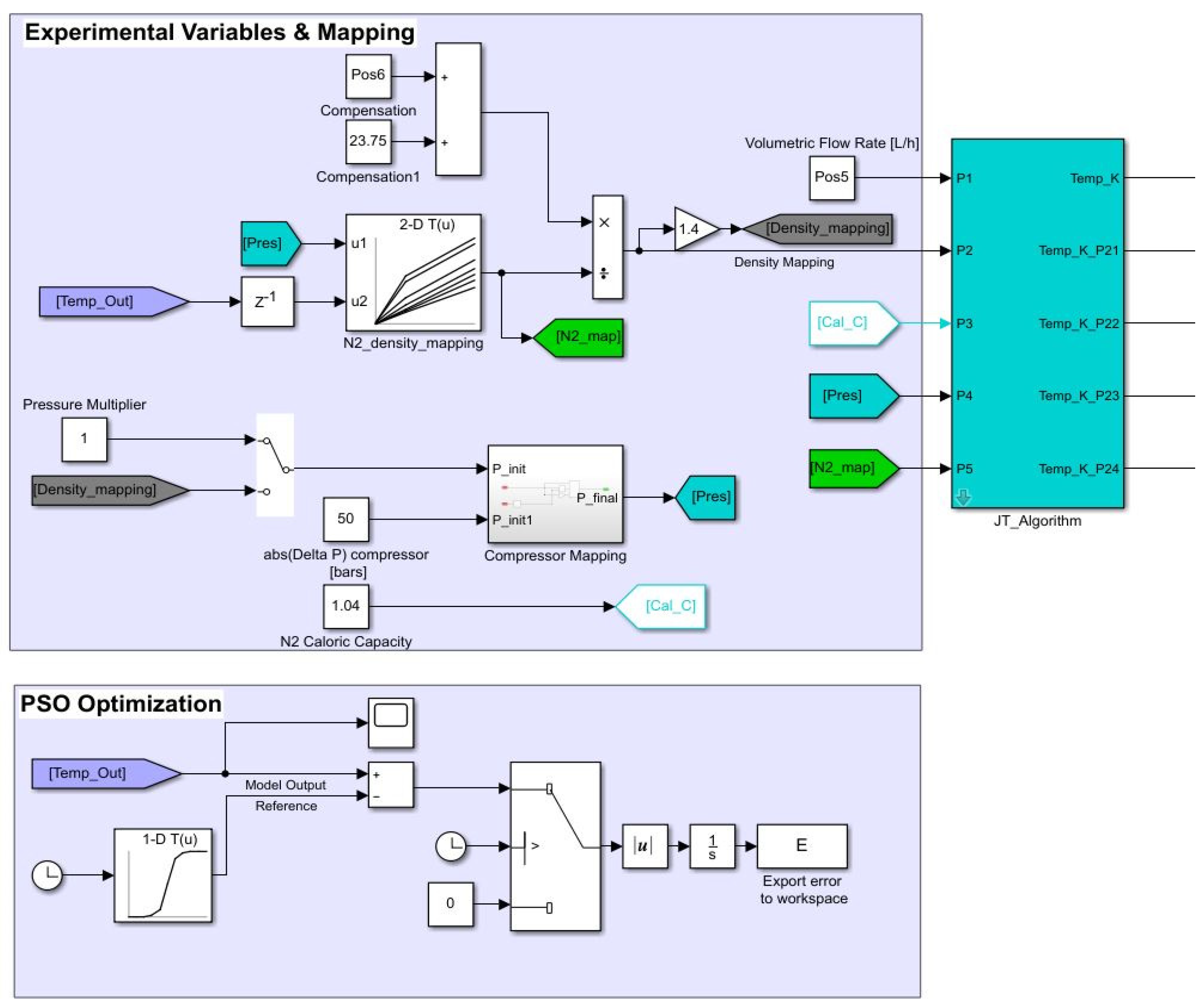
Figure 13, the resulting Hampson-Linde cryogenic cooler model diagram is presented. The schematic from this figure is linked to the Simulink/Simscape model from
Figure 14, where all sections were highlighted.
The following sections can be distinguished from
Figure 14:
Pressurized gas heat transfer;
External heat exchange;
External heat exchange;
Heat exchanger heat transfer;
Infinite resistance was used to set the bias (initial point of simulation) of temperature to the ambient temperature;
Decompressed gas heat transfer;
Decompression at the Joule-Thomson valve.
The previous part of the model was used to predict the temperature change, while the part from
Figure 15 modeled the behavior of decompression and other prototypes previously implemented during experimental stages.
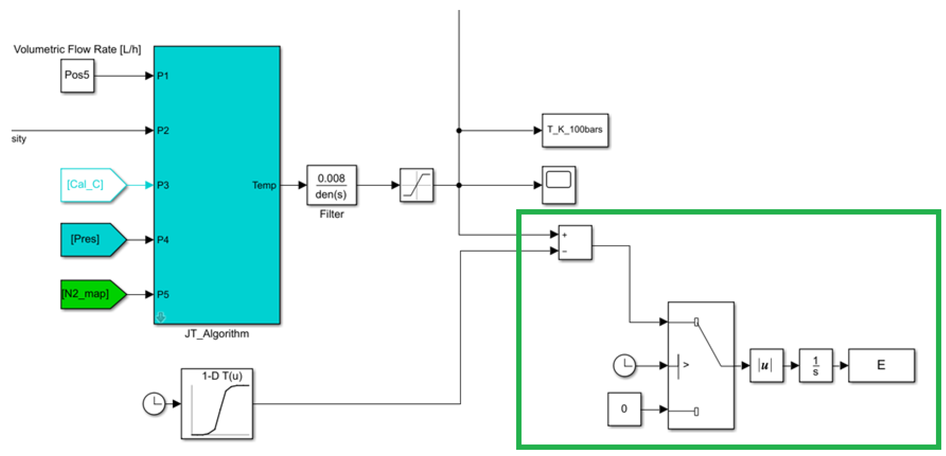
As for the optimization criteria, the heuristic optimization was run to superimpose the model’s output characteristic with a reference signal, an asymptotic signal which decreased gradually to a target value. The section used in determining the objective function value through the absolute value of an integral is presented below in
Figure 16, highlighted in green.
The output temperature characteristic is presented below in
Figure 17. The chart shows an asymptotic decrease in temperature at the Joule-Thomson valve, which corresponded to a heat transfer model based on differential equations. Due to the absence of data from
Figure 12, the linear lookup table extrapolation caused the last illustrated characteristic to vary non-linearly.
The superconductive reference compound was Y-Ba-Cu-O, having a critical temperature of 92 K [
19]. The previously presented result showed that the superconductive state for this category II superconductor could be obtained since its temperature was below the previously mentioned value.
All values resulting from the particle swarm optimization algorithm are listed below in
Table 2.
Comparing the obtained characteristics and results with studies mentioned in [
20], even with the limitation, which will be further discussed within the next section, results were comparable to cryogenic coolers using all or any Brayton cycle, Claude and Kapitza cycle.
Figure 17 and
Figure 18 show a characteristic that opposed external heat transfer (non-adiabatic gas expansion) and an adiabatic gas expansion temperature characteristic.
Following the description of the prototype model and results after PSO, consistent results were obtained from a heat transfer point of view, for example, high thermal resistor values for external heat exchanger and cooling dynamics corresponding to existing studies. However, several limitations occurred using these methods, covered in the next section.
4. Discussion
4.1. General Aspects
Further validation of this methodology and model would be made by comparing and optimizing the model based on a real, physical prototype. The values found by the parallel PSO algorithm represent discretized components. Based on the obtained values after optimization, one could determine the correctness of model implementation only by comparing the obtained values with mathematical estimations, due to the absence of physical data. A certain tolerance would result because two translations were made, from which one was for complexity reduction, allowing the PSO algorithm to provide an acceptable output for a discrete model, with a smaller number of parameters (whose values were used multiple times due to discretization), in a reduced amount of time. Also, another nonlinearity occurred due to the mathematics from Ohm’s Law adapted for thermal circuits.
4.2. Limitations
4.2.1. The Parallel PSO Algorithm
While maintaining a constant particle (optimizing agent) density along individual axes, the total time required to finish one iteration increased exponentially, as shown in
Figure 19. During PSO, each optimization variable defined one dimension and had “N” parameters to optimize for every model. One can say the optimizing agents searched inside an N-dimensional space.
As shown above, a limitation of each heuristic algorithm occurred due to the agents moving through the searching space defined by a certain number of dimensions. Multiple variables could be optimized without having this issue, only by grouping them when implementing discrete models.
4.2.2. Mathematical Model
In contrast to a Joule-Thomson valve, this component was modeled as a translated current source, or power dissipation source, during the current implementation. This power dissipation source implemented a Peltier element, as shown below in
Figure 20, since, between the two points of heat transfer, no heat exchange took place through this component.
One main difference between the actual functionality and the implemented solution is that, by choosing the same thermal resistor value overall pressure lines, a temperature increase occurred for probes P1.1 to P1.4. In contrast, probes’ values would indicate a temperature below the ambient value in a real Hampson-Linde topology. This suggests better results would be obtained by further dividing and grouping the model variables and improving the throttle valve model.
Moreover, the Joule-Thomson coefficient gives the maximum temperature difference before and after the valve in a Hampson-Linde system. As an ideal decompression, power dissipation was described from Equation (9), and due to both variable grouping and functional dissimilarity, dissipated power caused a temperature deviation in the high-pressure line. However, as shown below in
Figure 21, consistent results were obtained for the low-pressure line.
Overall, consistency in results was maintained except for the high-pressure line, for which occurring deviations were mentioned and explained, occurring because of discrete variables grouped over all gas heat transfer contribution prototypes, and due to the throttle valve model.
5. Conclusions
First, in contrast to other models based on adiabatic liquid storage during the liquefaction process, the presented study involved implementing a non-adiabatic process-based decompression, predicting a physical prototype behavior more accurately upon further optimizing. However, modeling such a process with thermodynamic equations also allows considering the phase transition, whereas further improvement would be needed to model such a factor in the black box Simulink model.
The initial step in developing the Hampson-Linde cryogenic cooler model was implementing a parallel PSO algorithm. A prototype model was developed afterward, based on Ohm’s Law for thermal circuits, which discretized thermal transfer, followed by two mathematical simplifications—the thermal to electric domain transfer for components and the time domain model translation for heat transfer. However, a certain tolerance would occur between the actual model and the physical implementation using these two translations and resulting from grouping the discrete optimized parameters. Also, since the model was optimized using data based on estimations for discrete components, further calibration would be needed compared with real prototypes.
Once a model predicted such temperature characteristics, a superconductive state for category II superconductors could be predicted in materials used in more complex concepts, such as the Hyperloop concept and other applications which use similar requirements. Last, but not least, further validation of this methodology would be implementing a lambda-point generator cryogenic cooler for category I superconductors.
Author Contributions
Conceptualization, methodology, validation, supervision, project administration, funding acquisition, review and editing was done by L.A.S.; Conceptualization, methodology, validation, software, investigation, data curation, writing—original draft preparation, visualization was done by M.A.C. All authors have read and agreed to the published version of the manuscript.
Funding
This research was funded by the Romanian Ministry of Education and Research, grant number PN-III-P2-2.1-PED-2019-2601, “REGRENPOS”.
Conflicts of Interest
The authors declare no conflict of interest.
References
- Snitchler, G. Progress on High Temperature Superconductor Propulsion Motors and Direct Drive Wind Generators. In Proceedings of the 2010 International Power Electronics Conference—ECCE ASIA, Sapporo, Japan, 21–24 June 2010; pp. 5–10. [Google Scholar] [CrossRef]
- Tipparach, U. Fabrication of And Transport Studies On YBa2Cu3O7/PrBa2(Cu1-xMx)3O7 Type Multilayers. Ph.D. Thesis, University of North Dakota, Grand Forks, ND, USA, 2002. [Google Scholar] [CrossRef]
- Winnefeld, C.; Kadyk, T.; Bensmann, B.; Krewer, U.; Hanke-Rauschenbach, R. Modelling and Designing Cryogenic Hydrogen Tanks for Future Aircraft Applications. Energies 2018, 11, 105. [Google Scholar] [CrossRef] [Green Version]
- Paglini, R.; Gandiglio, M.; Lanzini, A. Technologies for Deep Biogas Purification and Use in Zero-Emission Fuel Cells Systems. Energies 2022, 15, 3551. [Google Scholar] [CrossRef]
- Ichkitidze, L.P.; Belodedov, M.V.; Gerasimenko, A.Y.; Telyshev, D.V.; Selishchev, S.V. Possibility Noninvasive Detection Magnetic Particles in Biological Objects. Eng. Proc. 2021, 6, 61. [Google Scholar] [CrossRef]
- Hartmann, C.; Nøland, J.K.; Nilssen, R.; Mellerud, R. Dual Use of Liquid Hydrogen in a Next-Generation PEMFC-Powered Regional Aircraft with Superconducting Propulsion. IEEE Trans. Transp. Electrif. 2022. [Google Scholar] [CrossRef]
- Bizon, N.; Carcadea, E.; Iliescu, M.; Raboaca, M.S.; Manta, I.; Sorlei, S.I. Estimation of Hydrogen Consumption for Proton-Exchange Membrane Fuel Cells Systems. In Proceedings of the 2021 13th International Conference on Electronics, Computers and Artificial Intelligence (ECAI), Pitesti, Romania, 1 July 2021; pp. 1–7. [Google Scholar] [CrossRef]
- Wood, T.S.; Graber, V. Superconducting Phases in Neutron Star Cores. Universe 2022, 8, 228. [Google Scholar] [CrossRef]
- Huebener, R.P. The Path to Type-II Superconductivity. Metals 2019, 9, 682. [Google Scholar] [CrossRef] [Green Version]
- Fagaly, R. Superconducting quantum interference device instruments and applications. Rev. Sci. Instrum. 2006, 77, 101101. [Google Scholar] [CrossRef] [Green Version]
- Oyama, H.; Shinzato, T.; Hayashi, K.; Kitajima, K.; Ariyoshi, T.; Sawai, T. Application of superconductors for automobiles. SEI Tech. Rev. 2008, 67, 22–26. [Google Scholar]
- Lim, J.; Lee, C.; Choi, S.; Lee, J.; Lee, K. Design Optimization of a 2G HTS Magnet for Subsonic Transportation. IEEE Trans. Appl. Supercond. 2020, 30, 1–5. [Google Scholar] [CrossRef]
- Cheema, M.A.M.; Fletcher, J.E.; Xiao, D.; Rahman, M.F. A Direct Thrust Control Scheme for Linear Permanent Magnet Synchronous Motor Based on Online Duty Ratio Control. IEEE Trans. Power Electron 2016, 31, 4416–4428. [Google Scholar] [CrossRef]
- El-Shorbagy, M.; Hassanien, A.E. Particle Swarm Optimization from Theory to Applications. Int. J. Rough Sets Data Anal. 2018, 5, 1–24. [Google Scholar] [CrossRef]
- Flores-Livas, J.A.; Boeri, L.; Sanna, A.; Profeta, G.; Arita, R.; Eremets, M. A per-spective on conventional high-temperature superconductors at high pressure: Methods and materials. Phys. Rep. 2020, 856, 1–78. [Google Scholar] [CrossRef]
- Windmeier, C.; Barron, R. Ullmann’s Encyclopedia of Industrial Chemistry: Cryogenic Technology; Wiley-VCH Verlag GmbH & Co. KGaA: Weinheim, Germany, 2013; pp. 1–71. [Google Scholar] [CrossRef]
- Lerou, P.P.P.M.; Jansen, H.V.; Venhorst, G.C.F.; Burger, J.; Veenstra, T.; Holland, H.J.M.; Brake, H.J.M.; Elwenspoek, M.; Rogalla, H. Progress in Micro Joule-Thomson Cooling at Twente University; Springer: Boston, MA, USA, 2005; Volume 13, pp. 489–496. [Google Scholar] [CrossRef]
- Dadsetani, R.; Sheikhzadeh, G.A.; Safaei, M.R.; Alnaqi, A.A.; Amiriyoon, A. Exergoeconomic optimization of liquefying cycle for noble gas argon. Heat Mass Transf. 2019, 55, 1995–2007. [Google Scholar] [CrossRef]
- Gholipour, S.; Daadmehr, V.; Rezakhani, A. Khosroabadi, H. Shahbaz, F.; Akbarnejad, R. Structural Phase of Y358 Superconductor Comparison with Y123. J. Supercond. Nov. Magn. 2012, 25, 2253–2258. [Google Scholar] [CrossRef]
- Yang, S.; Liu, Z.; Fu, B. Simulation and Evaluation on the Dynamic Performance of a Cryogenic Turbo-Based Reverse Brayton Refrigerator. Appl. Sci. 2019, 9, 531. [Google Scholar] [CrossRef] [Green Version]
Figure 1.
Superconductive characteristic of mercury [
2].
Figure 1.
Superconductive characteristic of mercury [
2].
Figure 2.
Magnetic field lines around normal state conductor and superconductive state conductor. (a) A temperature higher than the critical temperature of a superconductor does not influence magnetic field lines; (b) During the superconductive state, magnetic field lines induce a surface current through the superconductor. This leads to magnetic levitation, since incident magnetic field lines are expelled.
Figure 3.
A comparison between a conventional electric vehicle and a vehicle using a superconductive electric motor. (a) Block diagram for conventional electric vehicles; (b) Possible topology for superconductive motor electric vehicles.
Figure 3.
A comparison between a conventional electric vehicle and a vehicle using a superconductive electric motor. (a) Block diagram for conventional electric vehicles; (b) Possible topology for superconductive motor electric vehicles.
Figure 4.
Hyperloop concept [
12].
Figure 4.
Hyperloop concept [
12].
Figure 5.
Illustration of PSO algorithm principles and mathematical description.
Figure 5.
Illustration of PSO algorithm principles and mathematical description.
Figure 6.
Pressure to temperature chart of a real gas [
16].
Figure 6.
Pressure to temperature chart of a real gas [
16].
Figure 7.
Hampson-Linde cryogenic cooler functional diagram [
17].
Figure 7.
Hampson-Linde cryogenic cooler functional diagram [
17].
Figure 8.
Parallel PSO algorithm block diagram.
Figure 8.
Parallel PSO algorithm block diagram.
Figure 9.
Global best cost value over several iterations for the previous function.
Figure 9.
Global best cost value over several iterations for the previous function.
Figure 10.
Prototype of gas heat transfer contribution.
Figure 10.
Prototype of gas heat transfer contribution.
Figure 11.
Prototype of the heat exchanger contribution.
Figure 11.
Prototype of the heat exchanger contribution.
Figure 12.
Nitrogen density as a function of pressure and temperature.
Figure 12.
Nitrogen density as a function of pressure and temperature.
Figure 13.
Hampson-Linde process block diagram.
Figure 13.
Hampson-Linde process block diagram.
Figure 14.
Simulink/Simscape model of the Joule-Thomson-based cryogenic cooler process. Three sections of discrete heat exchanger thermal transfer can be distinguished, each containing a thermal capacitance. All corresponding sections are explained below.
Figure 14.
Simulink/Simscape model of the Joule-Thomson-based cryogenic cooler process. Three sections of discrete heat exchanger thermal transfer can be distinguished, each containing a thermal capacitance. All corresponding sections are explained below.
Figure 15.
Density mapping and decompression behavior. All outputs were filtered using first order filters for further smoothing of characteristics, having the first filtered output, “Temp_K”, corresponding to the “Temp_Out” tag.
Figure 15.
Density mapping and decompression behavior. All outputs were filtered using first order filters for further smoothing of characteristics, having the first filtered output, “Temp_K”, corresponding to the “Temp_Out” tag.
Figure 16.
Optimization criteria.
Figure 16.
Optimization criteria.
Figure 17.
Cooling characteristic of the model prototype at expander outlet.
Figure 17.
Cooling characteristic of the model prototype at expander outlet.
Figure 18.
Turbo-compressor-based refrigerator dynamic cooling characteristic [
20].
Figure 18.
Turbo-compressor-based refrigerator dynamic cooling characteristic [
20].
Figure 19.
Maintaining a constant optimizing density of 3 agents per axis versus total optimizing time. In this case, a significant increase in optimizing time occurs for a linear increase in the number of particles, limiting the number of variables that can be optimized. Simulation time is 0.1 s, while the total time is shown for one single iteration of PSO.
Figure 20.
Thermal analysis and further functionality description of the prototype. Gradient intensity shows the temperature difference in comparison with ambient temperature. The red color shows temperatures above ambient value, while blue shows temperatures below ambient. All heat exchanger discrete sections correspond to
Figure 14.
Figure 21.
End of simulation temperature values for probes P2.1 to P2.4 function of input pressure and proximity towards the decompression point. An increase in proximity corresponds to an even closer probe towards the Joule-Thomson throttle valve.
Figure 21.
End of simulation temperature values for probes P2.1 to P2.4 function of input pressure and proximity towards the decompression point. An increase in proximity corresponds to an even closer probe towards the Joule-Thomson throttle valve.
Table 1.
Electrical to thermal domain translation.
Table 1.
Electrical to thermal domain translation.
| Physical Variable | Description | Measurement Unit |
|---|
| Q | Heat transfer rate | J (Joule) |
| T | Temperature | K (Kelvin degree) |
| Rth | Thermal resistance | K/W (Kelvin per watt) |
| Cth | Thermal capacitance | J/K (Joule per Kelvin) |
| c | Specific heat capacity | J/kgK (Joule per kilogram Kelvin) 1 |
Table 2.
Cryogenic cooler model parameters.
Table 2.
Cryogenic cooler model parameters.
| Parameter | Value |
|---|
| Nitrogen thermal resistance | 8.0540612 K/W |
| Heat exchanger internal thermal capacitance | 7.1426119 J/K (428.556714 J/K) 1 |
| Heat Exchanger internal thermal resistance | 53.550687 K/W |
| External heat exchange thermal resistance | 9135.2208 K/W |
| Compressor volumetric flow | 3682.3641 L/h |
| Square of compensation density | 33.2700 (kg/m3)2 2 |
| Publisher’s Note: MDPI stays neutral with regard to jurisdictional claims in published maps and institutional affiliations. |
© 2022 by the authors. Licensee MDPI, Basel, Switzerland. This article is an open access article distributed under the terms and conditions of the Creative Commons Attribution (CC BY) license (https://creativecommons.org/licenses/by/4.0/).


