Application of Statistical Process Control for Structural Health Monitoring of a High-Speed Railway Track System

Abstract

To make full use of the massive monitoring data accumulated in China high-speed railways, an improved statistical process control (SPC) framework was introduced to analyze the discontinuous monitoring data of the track system on a high-speed railway elevated station. Multilinear regression models and time series difference equation (TSDE) models were first developed to separate common-cause variations in the monitoring data. Then, individual control charts, moving range control charts, and exponentially weighted moving average control charts were constructed to detect special-cause variations. Results showed that the variations of girder displacement and track slab–girder relative displacements mainly resulted from temperature effects and linear trends related with material damages. Moreover, visible serial dependence was found in the regression model residuals, which could be effectively captured by the TSDE model. Numerous outliers were detected at the measuring points of rail–track slab displacement 15 and track slab–girder relative displacement 17 by more than three control charts, implying higher sensitivity to special causes. With respect to the special causes triggering the anomalous responses of local and overall track systems, sixteen and twenty-eight significant special events were detected, respectively.

1. Introduction

High-speed railways have been widely applied in various countries during the past several decades. Compared with normal-speed railways, the high-speed railways place high requirements on track systems. Under the actions of external factors such as cyclic temperature loadings and train impact loadings, various diseases easily emerge in the parts of the track systems during operation [1,2]. To ensure safe operation, several monitoring systems have been constructed to monitor the service status of track systems in real time. Massive monitoring data were accumulated in this process [3,4,5]. Due to a range of reasons, including external environmental actions, poor installation, and hardware problems, data loss occurred during wireless transmission and led to lots of discontinuous monitoring data [6,7,8,9]. Data loss decreases the quality of analysis results and adds challenges to the data processing and analysis. Researchers have proposed several methods to recover the data loss, including acknowledgments [10,11], forward error correction [12], convolutional neural networks [13], compressive sensing [8,9], etc. However, these methods are effective only under certain conditions. The in-depth analysis and full utilization on discontinuous data play essential roles in optimizing monitoring technology, evaluating the service status and prolonging the life of track systems [14,15].

A statistical process control (SPC) framework was proposed to fulfil the efficient monitoring and management of structures. The framework was built based on the SPC notion [16,17], in which changes in the output of a stochastic process consist of common- cause variation, special-cause variation, and inherent random variation. In the case of a track system, the common-cause variation is produced by usual environmental and operational conditions, such as normal weather and train loadings. The special-cause variation is attributed to special events, including extreme weather, unusual loads, structural damage, etc. The inherent random variation is related to the cumulative effects of many small, unavoidable causes [18]. Importantly, the detection of special events could deepen the understanding of decision-makers on the monitoring data, thereby initiating immediate management of infrastructure [19].

In the past several decades, SPC has been widely applied in the structural health monitoring (SHM) of civil engineering infrastructure [19,20,21,22,23,24,25]. Sohn et al. [20] applied an X-bar control chart of SPC in the vibration-based damage diagnosis of a concrete bridge column. Fugate et al. [21] utilized an autoregressive (AR) model to fit the acceleration time histories of a concrete bridge column and employed X-bar and S control charts to monitor the mean and variance of the AR model residual. Lu et al. [22] validated the damage detection ability of the Shewhart control chart based on the predamage and postdamage data of a bridge. Magalhães et al. [23] identified the damage of a concrete arch bridge with the construction of T² control charts. Chen et al. [24,25] developed a two-part SPC framework to excavate the continuous monitoring data of the Hurley Bridge, that is, separating common-cause variation by using statistical models at first and then detecting special-cause variation with the use of univariate and multivariate control charts. Kosnik et al. [19] extended the two-part SPC framework and analyzed continuous delamination data of the Grace Church building. However, so far, little research has used the SPC framework to analyze the discontinuous monitoring data of high-speed railway track systems.

Responses of track systems include static and dynamic responses determined by whether the trains pass by or not. Evaluation of the anomalies in track systems by dynamic responses is featured with high sensitivity but also high complexity. Moreover, the train impacting in a turnout leads to relatively large dynamic responses [26], which brings interference to data analysis. Therefore, this paper focuses on the output-only monitoring of track systems in static condition, with emphasis on the long-term structural changes and sustainable anomalies.

In this study, the two-part SPC framework was improved by introducing a time series difference equation (TSDE) model to capture the serial dependence in monitoring sequences. Based on the improved SPC framework, discontinuous monitoring data of a high-speed railway track system were analyzed in depth. Firstly, the common-cause variations in the monitoring data were separated sequentially by multilinear regression models and TSDE models. Then, the special-cause variations in the monitoring data were detected by the control charts composed of individual control charts, moving range control charts, and exponentially weighted moving average (EWMA) control charts. Finally, the locations of the track system that are sensitive to special causes were recognized, and significant special events were determined. This study is expected to assist decision-makers to understand and excavate the monitoring data of railway track and provide a guidance for the maintenance of track systems.

2. Research Approach

2.1. Statistical Models

As mentioned above, the changes of monitoring data in track systems are induced by complex causes. Statistical models are developed to support the infrastructure management and focus on characterization of common-cause variation [24,25]. In this section, statistical models were used to control the common-cause variations in the monitoring data of a track system. In statistical models, multilinear regression models have been commonly used for time series analysis in civil structures [24,25,27,28,29]. It correlates the data variations with the changes in explanatory variables, thereby facilitating structural analysis of the influences of the explanatory variables on the structural responses. Thus, the multilinear regression model was first applied to explain the effects of temperature and linear trend on the response measurements. As carryover effects from earlier measurements, serial dependence can lead to common-cause variation unexplained by the regression model. Considering the strong discontinuity of monitoring data, the time series difference equation model was then utilized to capture the autocorrelation in the regression model residuals.

2.1.1. Multilinear Regression Model

Two or more independent variables were used in a multilinear regression model to represent the dependent variable linearly. Air temperature and linear trends were selected to be explanatory variables, and the regression equations are formulated as follows:

$$y_t={\beta }_0+{\beta }_{1}t+{\beta }_2{T}_t+{\in }_t,$$

(1)

where t = 1, …, t_max are used to indicate the days in the analysis period. $T_t$ corresponds to the average air temperature on day t. The coefficients ${\beta }_0$, ${\beta }_1$, and ${\beta }_2$ represent the intercept, the slope of the linear trend, and the slope of the air temperature, respectively. ${\in }_t$ denotes the residuals.

2.1.2. Time Series Difference Equation Model

The equation of the time series difference equation model is formulated as follows:

$${\in }_t={\phi }_0+{\sum }_{i=1}^p{\phi }_i·{ϵ}_{t-i}+x_t,$$

(2)

where t = 1, …, t_max are used to indicate the days in the analysis period. p represents the order of the time series difference equation. ${ϵ}_t, {ϵ}_{t-1}, \dots , {ϵ}_{t-p}$ correspond to the time t, t − 1, …, t − p regression model residuals. ${\phi }_i$ represents the coefficient of difference equation. $x_t$ is the residual of the difference equation.

2.2. Control Charts

In this section, control charts were used to detect the special-cause variations in the monitoring data of a track system. The control charts are graphical representations of the evolution of system quality characteristics with time. They are used to judge whether the system quality characteristics are in a stable state and to recognize the random fluctuation and abnormal fluctuation. A special-cause will lead to the deviation of statistical model residuals from the normal independent and identically distributed data generated by a stochastic process. Specifically, the deviation includes shifts and drifts, which refer to sudden/discrete changes and gradual/continuous changes, respectively. The control charts are designed to identify the shifts/drifts and thus detect the special events [24].

Firstly, individual control charts and moving range control charts were used to detect the deviations in the mean and variance of monitoring sequences, respectively. Supplementary runs rules were then used to detect abnormal sequences in the individual control chart, while EWMA control charts were used to detect small-amplitude continuous shifts or drifts during monitoring. Afterwards, special events were detected based on the analysis results of control charts.

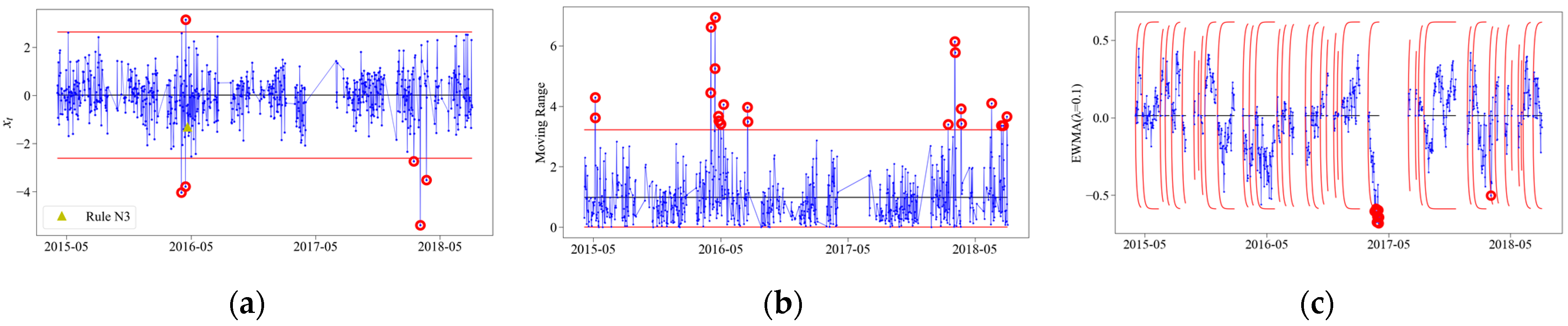
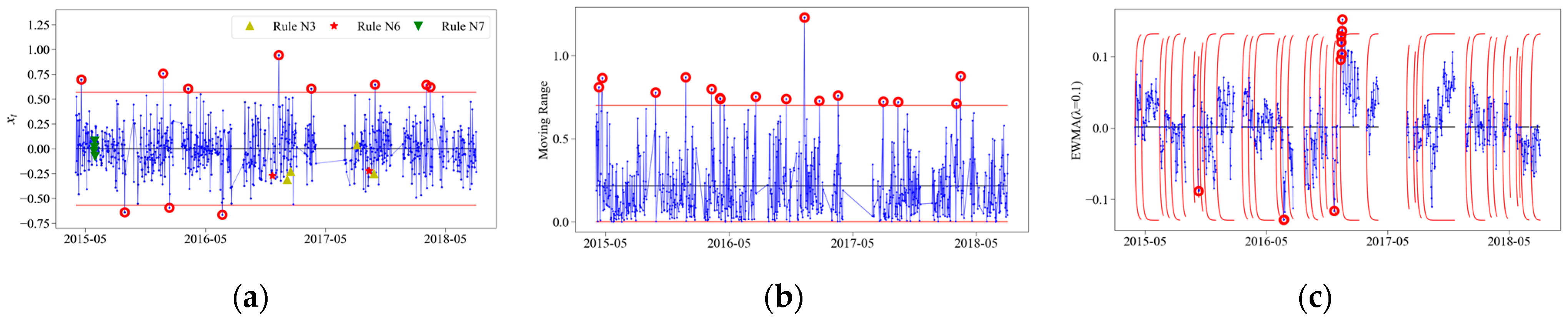
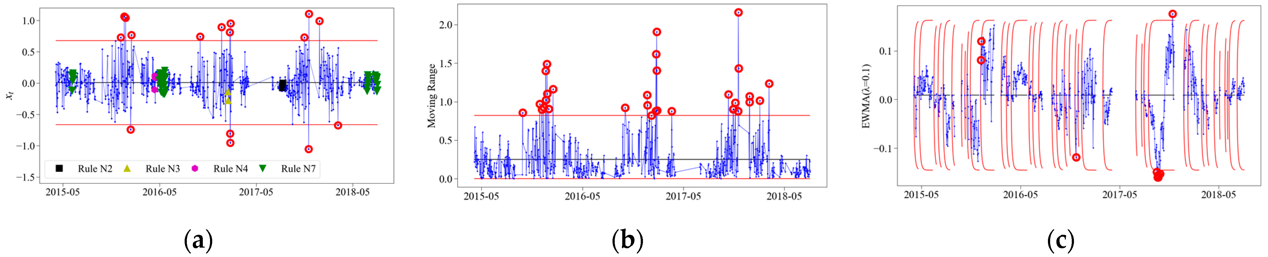
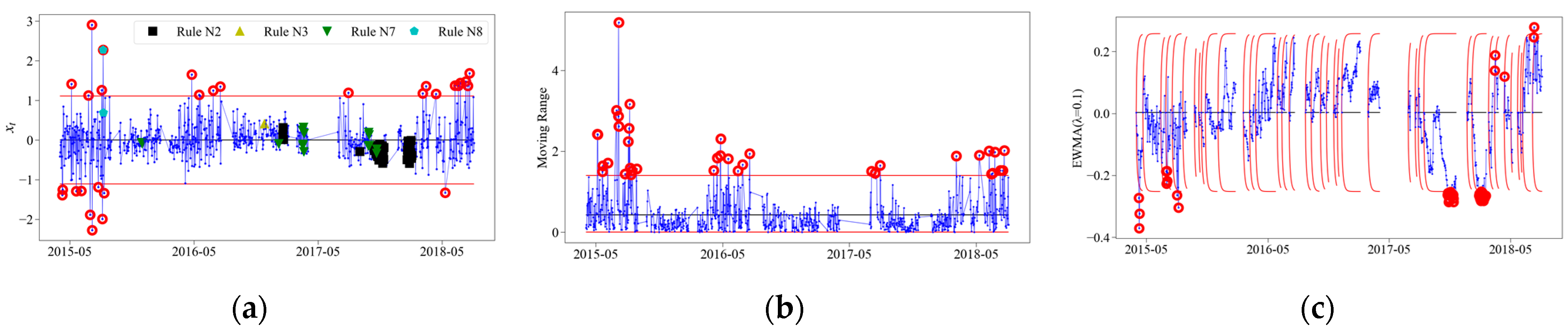
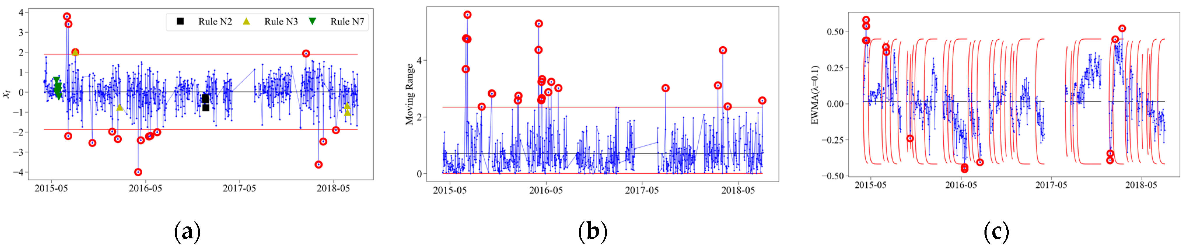
2.2.1. Individual Control Chart

The centerline (CL) of an individual control chart corresponds to the sample average.

$$\mathrm{CL}=\widehat{\mu }=\overline{x}=\frac{1}{T}{\displaystyle \sum }_{t=1}^T{x}_t$$

(3)

As described in reference [16], an unbiased estimate $\widehat{\sigma }$ of sample standard deviation is obtained as follows:

$$\widehat{\sigma }=\frac{\overline{\mathrm{MR}}}{d_2}$$

(4)

where ${\mathrm{MR}}_t=\left|x_t-x_{t-1}\right|$ is the individual moving range for the pair of consecutive measurements at t − 1 and t, and $\overline{\mathrm{MR}}={\displaystyle \sum }_{t=2}^T{\mathrm{MR}}_t/\left(T-1\right)$ is the mean individual moving range. When two consecutive measurements are used to calculate the moving ranges, d₂ = 1.128 [18].

Following common practice in SPC, a distance L from the CL is set to 3 to specify the upper and lower control limits of individual control charts, as follows:

$$\mathrm{UCL}=\widehat{\mu }+L\widehat{\sigma }$$

(5)

$$\mathrm{LCL}=\widehat{\mu }-L\widehat{\sigma }$$

(6)

2.2.2. Moving Range Control Chart

The reference line and upper and lower control limits of a moving range control chart are computed by

$$\mathrm{CL}=\overline{\mathrm{MR}}$$

(7)

$$\mathrm{UCL}=D_4-\overline{\mathrm{MR}}$$

(8)

$$\mathrm{LCL}=D_3-\overline{\mathrm{MR}}$$

(9)

where D₄ and D₃ are parameters relying on the number of measurements used to calculate the moving ranges MR_t. When two consecutive measurements are used to calculate the moving ranges, $D_4=3.27$, $D_3=0$ [18]. The control limits are designed so that interpretation of the chart is analogous to the individual control chart.

2.2.3. Supplementary Runs Rules

The supplementary runs rules are used to detect the abnormal sequence in the individual control charts, that is, the sustained shift or drift of the mean and variance of the measurement. Nelson [30] proposed eight runs rules for the individual control charts, as follows:

• Rule N1: 1 measurement above (or below) the upper (or lower) control limit.
• Rule N2: 9 consecutive measurements on one side of CL.
• Rule N3: 6 consecutive measurements increasing or decreasing.
• Rule N4: 14 consecutive measurements alternating up and down.
• Rule N5: 2 out of 3 measurements beyond CL ± $2\sigma$ on same side.
• Rule N6: 4 out of 5 measurements beyond CL ± $2\sigma$ on same side.
• Rule N7: 15 consecutive measurements between ±$1\sigma$ from CL.
• Rule N8: 8 consecutive measurements beyond CL ± $\sigma$ on both sides.

Rule N1 is the basic rule of the individual control chart to trigger the outliers. Rules N2–N8 are considered the supplementary detection of special events. Rules N2 and N3 are designed to detect sustained shifts and drifts in the means of monitoring sequences, respectively. Rule N4 is designed to detect the abnormal periodic changes of monitoring sequences. Rules N5–N8 are designed to detect sustained shifts in the variances of monitoring sequences.

2.2.4. EWMA Control Chart

The detection of small-magnitude (sustained) shifts or drifts indicating early damage is important. However, the individual control chart and moving range control chart cannot always identify these changes due to their reflection of sample information at a specific time. Hence, EWMA control charts with memory characteristics were implemented [24]. The EWMA control chart monitors the exponentially weighted moving-average value ${\mathrm{EWMA}}_t$ of the monitoring sequence. The ${\mathrm{EWMA}}_t$ is defined as

$${\mathrm{EWMA}}_t=\lambda ·x_t+\left(1-\lambda \right)·{\mathrm{EWMA}}_{t-1}$$

(10)

where $\lambda$ is an adjustable parameter to control the sensitivity of the EWMA control chart and its value is between 0 and 1. x_t is the measurement. ${\mathrm{EWMA}}_0$ is set to $\overline{x}$.

The reference levels of the EWMA control chart are given by

$$\mathrm{CL}=\overline{x}$$

(11)

$${\mathrm{UCL}}_t=\overline{x}+3\sigma ·\sqrt{\frac{\lambda }{2-\lambda }[1-{\left(1-\lambda \right)}^{2t}]}$$

(12)

$${\mathrm{LCL}}_t=\overline{x}-3\sigma ·\sqrt{\frac{\lambda }{2-\lambda }[1-{\left(1-\lambda \right)}^{2t}]}$$

(13)

where an unbiased estimate of $\sigma$ is as shown in Equation (4). Moreover, since $0<\lambda \le 1$, ${\left(1-\lambda \right)}^{2t}$ converges quickly to 0 as t increases. Therefore, the control limits converge to

$$\mathrm{UCL}=\overline{x}+3·\frac{\overline{MR}}{d_2}·\sqrt{\frac{\lambda }{2-\lambda }}$$

(14)

$$\mathrm{LCL}=\overline{x}-3·\frac{\overline{MR}}{d_2}·\sqrt{\frac{\lambda }{2-\lambda }}$$

(15)

Since the monitoring data of a track system are discontinuous, the exponentially weighted moving-average process is performed for each data segment and the ${\mathrm{EWMA}}_0$ of each data segment is set to the mean of whole monitoring data.

3. Data and Analysis

3.1. Acquisition and Preprocessing of Data

Monitoring data used here were collected from the long-term monitoring system of a No. 42 turnout near the Jin-Hu station of the Beijing–Shanghai high-speed railway. This area contains a track system of welded turnout, ballastless track, and continuous girder from top to bottom. Under the coupling actions of environmental factors and train loadings, premature degradation or damage emerges in the track system due to the complicated interaction between structures. Therefore, a long-term monitoring system of the track system was installed and operated in this area and its schematic is presented in Figure 1. One measuring point of air temperature, six measuring points of rail–track slab relative displacement, four measuring points of track slab–girder relative displacement and two measuring points of girder displacement were placed. All the measurements were monitored by the fiber Bragg grating sensors due to their advantages of lightweight, small size, high sensitivity, and so on [31]. The measurement accuracies of temperature and displacements are 0.1 °C and 0.1 mm, and the sampling interval is 15 min.

The analyzed temperature and displacement data were collected from 1 May 2015 to 2 September 2018. In summer and winter, the monitoring system has a potential risk of failure due to extremely high temperature and low temperature. Moreover, short-term artificial maintenance, failure of acquisition system, and interruption of transmission process also lead to short-term or long-term loss of monitoring data. Therefore, the raw data collected by the monitoring system need to be preprocessed. Firstly, the data with abnormal amplitudes are eliminated, including data with very large or very small amplitudes and flat signal data generated by the malfunction of sensors [32]. After removing these data with abnormal amplitude, four measuring points were abandoned because of few residual data, and only eight measuring points were reserved. Then, the daily data of the eight measuring points were averaged to form a new time series for analysis.

3.2. Analysis of Common-Cause Variation

3.2.1. Application of Multilinear Regression Model

The parameter estimation results of multilinear regression models are shown in

Table 1. Multilinear regression model: parameter estimates.

Measuring Point	Abbreviation	Intercept		Linear Trend		Air Temperature		R2
		${\mathbf{\beta }}_{\mathbf{0}}$	t-stat	${\mathbf{\beta }}_1$	t-stat	${\mathbf{\beta }}_2$	t-stat
Rail–track slab relative displacement 10	R-S-R-D10	6.3372	55.5	0.0025	18.4	−0.2355	−51.8	0.767
Rail–track slab relative displacement 13	R-S-R-D13	−0.5130	−10.2	−0.0001	−2.3	0.0394	19.7	0.308
Rail–track slab relative displacement 14	R-S-R-D14	−1.0387	−24.4	−0.0002	−4.3	−0.0228	−13.5	0.196
Rail–track slab relative displacement 15	R-S-R-D15	−0.6734	−20.1	−0.0011	−26.8	0.0341	25.6	0.591
Track slab–girder relative displacement 16	S-G-R-D16	−23.0683	−91.5	−0.0040	−13.5	0.9166	91.4	0.906
Track slab–girder relative displacement 17	S-G-R-D17	−6.4153	−123.9	−0.0009	−15.5	0.2408	117.0	0.940
Track slab–girder relative displacement 18	S-G-R-D18	10.2280	98.2	0.0017	13.7	−0.4057	−97.9	0.917
Girder displacement 21	G-D21	57.5937	145.6	0.0154	33.2	−2.0303	−129.1	0.952

. All absolute values of t-stat are larger than 1.96, indicating that corresponding variables are statistically significant at a 95% confidence level. In terms of fit goodness, the R² in the models of S-G-R-D16, S-G-R-D17, S-G-R-D18, and G-D21 are over 0.9, which means that the variations of monitoring data are mainly caused by temperature effects and linear trends. The R² of the models for the remaining measuring points are between 0.15 and 0.80, which may be related to the direct train loadings on rails.

Taking the girder displacement 21 (G-D21) in Figure 2 as an example, a monitoring sequence can be decomposed into a linear trend, temperature effect, and residual, according to the multilinear regression model. During the whole period of analysis, the girder at G-D21 moves to one side at an average speed of 0.0154 mm/day. The displacement variations of the observation are consistent with the one caused by the temperature effect, which indicates that the temperature is a key factor for the displacement variation at G-D21.

The total data variations caused by the linear trend and temperature effect are calculated as Equations (16) and (17). The results for four measuring points closely related to the temperature effects together with linear trends are listed in

Table 2. Comparison of total data variations caused by the linear trends and temperature effects.

Measuring Point	Data Variation Caused by the Linear Trend (mm)	Data Variation Caused by the Temperature Effect (mm)	Proportion (%)
S-G-R-D16	4.884	42.426	11.51%
S-G-R-D17	1.099	11.146	9.86%
S-G-R-D18	2.076	18.778	11.05%
G-D21	18.803	93.975	20.01%

. The proportions of data variations caused by the linear trends to the ones caused by the temperature effects almost exceed 10%, suggesting that linear trends are also unneglectable components of the measurement sequences. The linear trends may be related to the changes of material properties [24], including concrete creep in the girder, the aging and deterioration of girder bearings, etc. Moreover, the proportion at G-D21 is the largest and demonstrates that the changes of material properties have more effects on the rail–track slab relative displacement than the track slab–girder relative displacement.

$$D_{\mathrm{LT}}={\beta }_1\times T$$

(16)

$$D_{\mathrm{TT}}={\beta }_2\times {\Delta }_T$$

(17)

where $D_{\mathrm{LT}}$ and $D_{\mathrm{TT}}$ are the total data variations explained by the linear trend and temperature effect, respectively. $T$ is the whole period of analysis and ${\Delta }_T$ is the difference between maximum and minimum temperatures throughout the whole period of analysis.

3.2.2. Application of Time Series Difference Equation Model

The monitoring data of the track system are discontinuous, so the autocorrelation, partial autocorrelation, Akaike’s information criteria, and Bayesian information criteria are no longer suitable for selecting the order of difference equation. The coefficient of R² is adopted as the selection standard of model order and should satisfy the following two conditions: (1) the variation of R² with the model order is stable; (2) the t-stat of each coefficient is greater than 1.96 (with 95% significance level). When the R² of the model is greater than 0.7, the first order of R² > 0.7 is selected. Since the monitoring data of the track system were averaged, the remnant effects of early measurements are relatively small. The lowest order of the model should be selected once the above conditions are achieved. Figure 3 presents the relationship between R² and the order of the difference equation model. The model order of each measuring point is selected as 3, 1, 1, 3, 1, 1, 1, 1. The parameter estimation results of the time series difference equation models are shown in

Table 3. Time series difference equation model: parameter estimates.

Measuring Point	${\mathbf{\phi }}_1$	t-stat	${\mathbf{\phi }}_2$	t-stat	${\mathbf{\phi }}_3$	t-stat	R2
R-S-R-D10	0.8562	23.943	−0.2224	−4.854	0.1348	3.813	0.596
R-S-R-D13	0.9586	96.654	-	-	-	-	0.919
R-S-R-D14	0.9233	67.120	-	-	-	-	0.845
R-S-R-D15	0.8964	25.545	−0.3436	−7.484	0.2429	7.156	0.616
S-G-R-D16	0.8565	48.274	-	-	-	-	0.738
S-G-R-D17	0.7028	29.630	-	-	-	-	0.515
S-G-R-D18	0.8159	42.707	-	-	-	-	0.688
G-D21	0.7227	32.142	-	-	-	-	0.555

.

Serial dependence in the regression residuals and difference equation residuals is evaluated by analyzing the corresponding autocorrelation functions (ACFs). The longest continuous segment (97 days) of the monitoring sequence is selected to verify the feasibility of the aforementioned method for capturing the serial dependence. Figure 4 shows the ACFs of the regression residuals and difference equation residuals for R-S-R-D13. In terms of a stationary and serially-independent time series, the values of ACF are small, with lag ≥ 1, and vary irregularly with lags. By comparison, the time series difference equation model effectively eliminates the autocorrelation in the monitoring data. In addition, the ACF values of the difference equation residuals fall mostly in the blue shaded area in Figure 4b. The blue shaded area represents the 95% confidence interval. Therefore, the existence of serial dependence in the difference equation residual is rejected with 95% confidence.

3.3. Analysis of Special-Cause Variation

3.3.1. Example of Control Chart

Figure 5 and Figure 6 show the individual control chart and moving range control chart for R-S-R-D13, where sixteen and twenty-two outliers are detected, respectively. For a stationary normal independent and identical distribution process, the individual control chart is expected to produce three outliers for each measuring point, and the moving range control chart is expected to produce eight outliers [24]. More detected outliers suggest the presence of special causes.

Figure 7 exhibits the individual control chart for R-S-R-D13 with supplementary runs rules. Rule N2 detects an upward shift in the mean of the monitoring sequence during April 2017. Rule N3 detects downward drifts in the mean of the monitoring sequence during June and December 2015, and February 2018. Rule N7 detects increases in the variance of the monitoring sequence occurring in October 2017 and July 2018. Rule N8 detects a decrease in the variance of the monitoring sequence occurring in September 2015.

The adjustable parameter of EWMA control charts can be customized in the range $0<\lambda \le 1$. The smaller the $\lambda$ is, the smoother the corresponding control chart. That is, more attention is paid to the sustained changes of the mean instead of outliers [24]. According to the characteristics of the required control chart and the discontinuous monitoring data of the track system, λ = 0.1 is selected. From the EWMA control chart with λ = 0.1 for R-S-R-D13 shown in Figure 8, it is noted that a small continuous shift from 19 September 2015 to 26 September 2015 is detected.

3.3.2. Analysis of All Measuring Points

Complying with the analysis process of the control charts for R-S-R-D13 in Section 3.3.1, the control charts for R-S-R-D10, R-S-R-D14, R-S-R-D15, S-G-R-D16, S-G-R-D17, S-G-R-D18, and G-D21 are presented in Figure 9, Figure 10, Figure 11, Figure 12, Figure 13, Figure 14 and Figure 15.

Table 4. Summary of control chart outliers.

Measuring Point	Individual Control Chart	Supplementary Runs Rules	Moving Range Control Chart	EWMA Control Chart	Total
R-S-R-D10	6	1	21	10	38
R-S-R-D13	16	18	22	8	64
R-S-R-D14	11	10	16	10	47
R-S-R-D15	16	64	31	10	121
S-G-R-D16	13	7	21	15	56
S-G-R-D17	29	67	37	43	176
S-G-R-D18	16	17	23	15	71
G-D21	14	31	24	10	79
Total	121	215	195	121	652

summarizes the outliers detected by the individual control chart, moving range control chart, and EWMA control chart (λ = 0.1). It is clearly seen that 121, 215, 195, and 121 outliers are, respectively, detected by the individual control charts, supplementary runs rules, moving range control charts, and EWMA control charts. According to the discussion in Section 2.2, the individual control chart, moving range control chart, and supplementary runs rules are expected to produce 19 outliers (878 × 8 × 0.0027), 63 outliers (878 × 8 × 0.009), and 163 outliers (878 × 8 × 0.02321) [33]. The detected outliers exceed the expected value obviously, which indicates the existence of special events. These special events change the mean and variance of the monitoring data. The numbers of outliers detected by control charts for R-S-R-D15 and S-G-R-D17 are much larger than those detected by control charts for other measuring points. This suggests that the track system at these two measuring points is sensitive to special causes, such as cold waves, extreme high temperatures, structural deterioration, and damage, and should be paid more attention.

To heighten the reliability of detection results, significant special events are further determined by using two methods. With regard to the special causes triggering anomalous responses of the local track system, significant special events are determined by outliers of at least three control charts or rules in Table 4 at each measuring point. Usually, it is easy for a special event to cause the outliers in two control charts (individual control chart and moving range control chart), whereas the simultaneous triggers of outliers in the three control charts or rules are rarely found. In that case, the overlap of various control charts increases the credibility of special events. A total of sixteen significant special events are determined and listed in

Table 5. Significant special events determined by outliers of at least three control charts or rules at each measuring point.

Measuring Point	Date	Control Charts	Measuring Point	Date	Control Charts
R-S-R-D10	2018.4.3	I, MR, EWMA	S-G-R-D17	2017.11.19	I, N2, N7
R-S-R-D13	2015.9.19	I, MR, EWMA		2017.11.20	I, N2, N7
R-S-R-D14	2017.1.9	I, MR, EWMA		2018.8.9	I, MR, EWMA
R-S-R-D15	2016.1.5	I, MR, EWMA	S-G-R-D18	2015.7.30	I, MR, EWMA
S-G-R-D16	2015.7.30	I, MR, EWMA		2015.11.6	I, MR, EWMA
	2015.8.5	I, MR, EWMA	G-D21	2015.7.30	I, MR, EWMA
R-S-R-D10	2015.7.30	I, MR, EWMA		2015.9.1	I, N3, EWMA
	2015.9.6	I, N8, MR		2015.11.6	I, MR, EWMA

.

As for the special causes triggering anomalous responses of the overall track system, significant special events are decided by outliers of the control charts at more than three measuring points. Detections of multiple sensors can effectively reduce the probability of outliers induced by sensor failure and increase the confidence of significant special events. A total of twenty-eight significant special events are determined and listed in

Table 6. Significant special events determined by outliers of the control charts at more than three measuring points.

Date	Measuring Points with Outliers Detected	Number of Measuring Points	Date	Measuring Points with Outliers Detected	Number of Measuring Points
2015.6.27~2015.6.29	R-S-R-D14, S-G-R-D16, S-G-R-D18, G-D21	4	2016.6.8	R-S-R-D10, R-S-R-D15, S-G-R-D16, S-G-R-D18, G-D21	5
2015.7.30~2015.7.31	S-G-R-D16, S-G-R-D17, S-G-R-D18, G-D21	4	2016.6.19	R-S-R-D15, S-G-R-D16, S-G-R-D18, G-D21	4
2015.8.4~2015.8.5	R-S-R-D13, S-G-R-D16, S-G-R-D17, S-G-R-D18, G-D21	5	2017.1.20	R-S-R-D13, R-S-R-D15, S-G-R-D18, G-D21	4
2015.8.6	S-G-R-D16, S-G-R-D17, S-G-R-D18, G-D21	4	2017.2.20	R-S-R-D13, R-S-R-D15, S-G-R-D16, G-D21	4
2015.9.1	S-G-R-D16, S-G-R-D17, S-G-R-D18, G-D21	4	2017.4.19	R-S-R-D10, R-S-R-D13, R-S-R-D15, S-G-R-D17	4
2016.1.23	R-S-R-D13, R-S-R-D14, R-S-R-D15, S-G-R-D16	4	2017.8.28	S-G-R-D16, S-G-R-D17, S-G-R-D17, G-D21	4
2016.1.24	R-S-R-D14, R-S-R-D15, S-G-R-D16, G-D21	4	2018.3.15	R-S-R-D10, S-G-R-D16, S-G-R-D17, S-G-R-D18, G-D21	5
2016.5.2~2016.5.3	R-S-R-D10, S-G-R-D16, S-G-R-D18, G-D21	4	2018.4.3	R-S-R-D10, R-S-R-D14, S-G-R-D16, S-G-R-D18, G-D21	5
2016.5.12~2016.5.13	R-S-R-D15, S-G-R-D16, S-G-R-D18, G-D21	4	2018.4.4	R-S-R-D10, R-S-R-D13, S-G-R-D16, S-G-R-D17, G-D21	5
2016.5.14	R-S-R-D10, S-G-R-D16, S-G-R-D18, G-D21	4	2018.4.21	R-S-R-D10, S-G-R-D16, S-G-R-D18, G-D21	4
2016.5.15	R-S-R-D10, S-G-R-D16, S-G-R-D17, S-G-R-D18, G-D21	5	2018.7.24	R-S-R-D13, R-S-R-D15, S-G-R-D17, S-G-R-D18	4

. Among them, the durations of significant special events from 27 June 2015 to 29 June 2015 and from 12 May 2016 to 15 May 2016 are more than three days, which should be paid special attention.

4. Conclusions

During the past several decades, statistical process control has been proven to support safe and efficient management and operations of transportation infrastructure. However, the existing research mainly applied the statistical process control to the analysis of continuous monitoring data. The high-speed railway track systems are large-span structures with complicated forms. In SHM of the track systems, data loss is an unavoidable consequence of wireless sensor networks. While several methods have been proposed to recover the data loss, reconstruction of signals is effective only under certain conditions. Hence, in this study, an improved SPC framework was introduced to analyze the discontinuous monitoring data of a high-speed railway track system. Based on this framework, common-cause variations in the discontinuous monitoring data were first separated by using statistical models, and special events were then detected by the utilization of control charts. The main conclusions are drawn as follows:

(1)

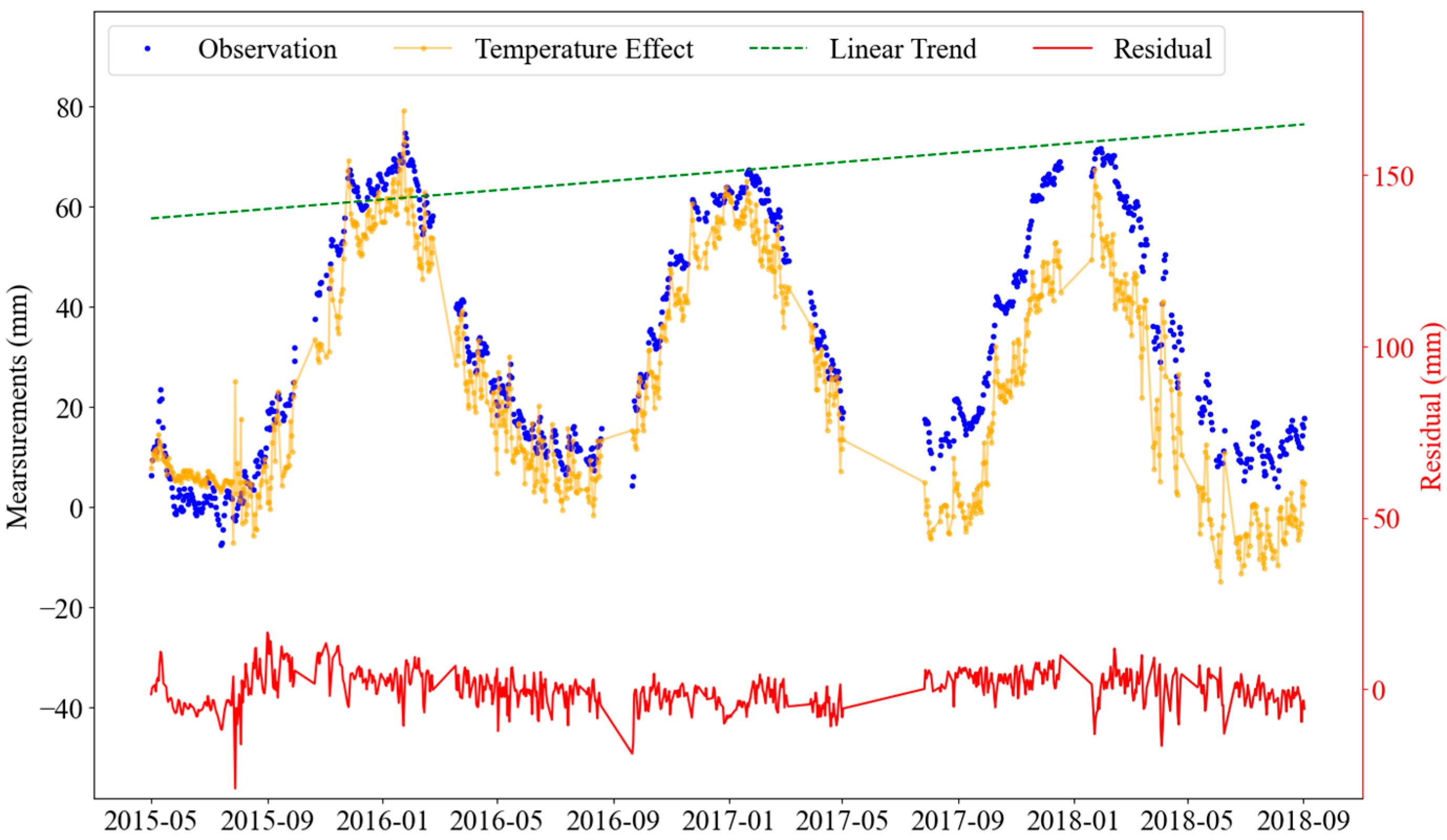
With respect to the girder displacement and track slab–girder relative displacements, the displacement variations were mainly caused by the temperature effects and linear trends. The variations of the observation were consistent with the one caused by the temperature effects, indicating that temperature is a key factor for the displacement variations. The proportions of these variations caused by the linear trends to the ones caused by the temperature effects almost exceed 10%, suggesting that linear trends were also unneglectable components in the measurement sequences.

(2)

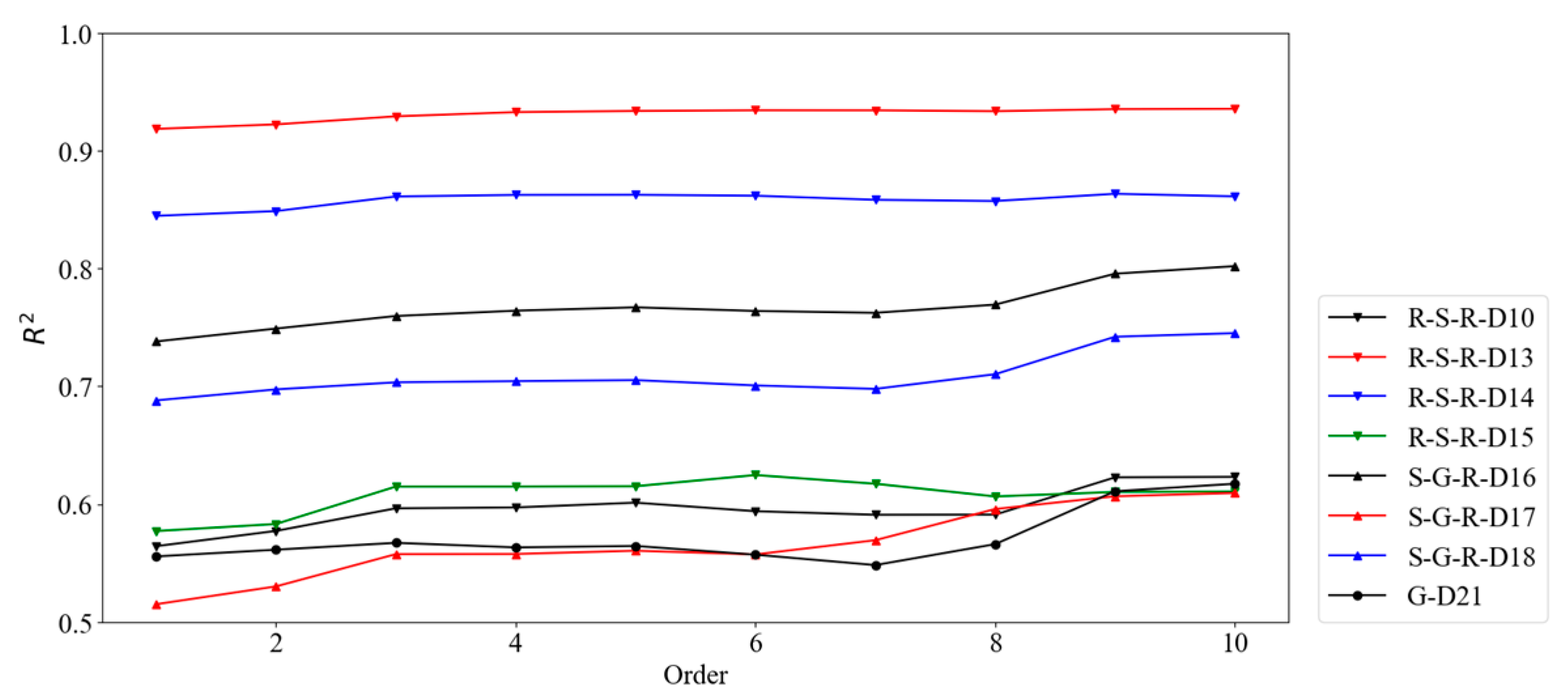
The ACF values of regression residuals were large with lag ≥ 1, and vary regularly with lags, indicating the serial dependence in the discontinuous monitoring data. The ACF values of difference equation residuals showed the opposite variation rules with lags, and fell mostly in the 95% confidence interval, which validates the feasibility of the TSDE model for capturing the serial dependence.

(3)

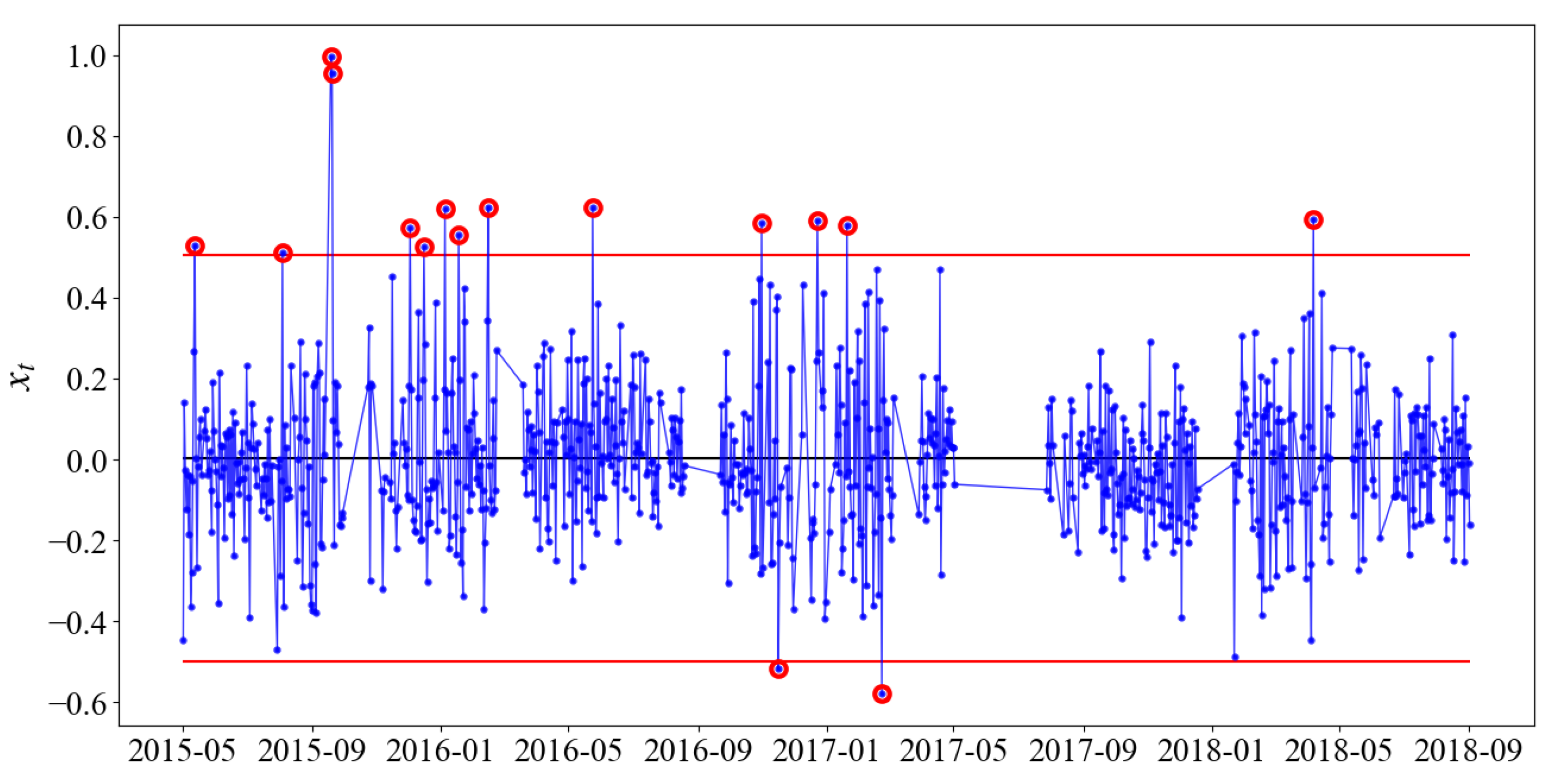
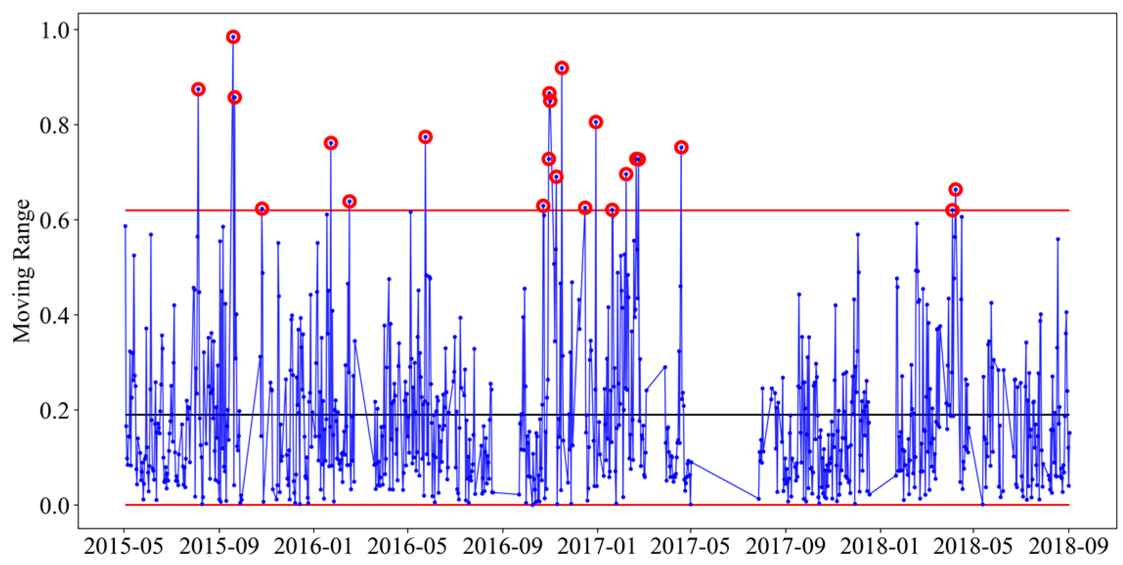
As for the rail–track slab relative displacement 15 and track slab–girder relative displacement 17, numerous outliers were detected by control charts. This suggested that the track system at these two measuring points was sensitive to special causes. With regard to the special causes triggering the anomalous responses of local and overall track systems, sixteen and twenty-eight significant special events were detected, respectively. Among these events, the durations of special events from 27 June 2015 to 29 June 2015 and from 12 May 2016 to 15 May 2016 exceeded three days, which should be paid special attention.

This improved SPC framework is necessary, for in the last years, several monitoring systems have been constructed for track systems. It can be used to explain the progression of measurements under ordinary conditions, and to detect special events generating automated alerts for online monitoring of SHM results. It is important to note that the developed framework is applicable for detection in static conditions. In order to be more suitable to other railway track systems, the framework here can be considered as a part of output-only monitoring. By integrating this framework with other analysis techniques (such as methods proposed by reference [34,35,36]), the information for the structural state will be collected more completely, and a more reliable SHM strategy of track systems may be promised.

References

1. Zhong, Y.L.; Gao, L.; Zhang, Y.R. Effect of Daily Changing Temperature on the Curling Behavior and Interface Stress of Slab Track in Construction Stage. Constr. Build. Mater. 2018, 185, 638–647. [Google Scholar] [CrossRef]
2. Cai, X.P.; Luo, B.C.; Zhong, Y.L.; Zhang, Y.R.; Hou, B.W. Arching Mechanism of the Slab Joints in CRTSII Slab Track under High Temperature Conditions. Eng. Fail. Anal. 2019, 98, 95–108. [Google Scholar] [CrossRef]
3. Cai, X.P.; Gao, L.; Liu, C.; Zhang, C.; Xin, T.; Sun, G.L. Monitoring Data Management Information System for Ballastless Track Turnout on Elevated Station. J. Railw. Eng. Soc. 2016, 33, 52–57. [Google Scholar]
4. Ye, X.W.; Ni, Y.Q.; Yin, J.H. Safety Monitoring of Railway Tunnel Construction Using FBG Sensing Technology. Adv. Struct. Eng. 2013, 16, 1401–1409. [Google Scholar] [CrossRef]
5. Ni, Y.Q.; Xia, H.W.; Ko, J.M. Structural Performance Evaluation of Tsing Ma Bridge Deck Using Long-Term Monitoring Data. Mod. Phys. Lett. B 2008, 22, 875–880. [Google Scholar] [CrossRef]
6. Wang, H.P.; Gong, X.S.; Wang, X.Z.; Feng, S.Y.; Yang, T.L.; Guo, Y.X. Discrete Curvature-Based Shape Configuration of Composite Pipes for Local Buckling Detection Based on Fiber Bragg Grating Sensors. Measurement 2022, 188, 110603. [Google Scholar] [CrossRef]
7. Gao, H.W.; Li, H.M.; Liu, B.; Zhang, H.; Luo, J.H.; Cao, Y.; Yuan, S.Z.; Zhang, W.G.; Kai, G.Y.; Dong, X.Y. A Novel Fiber Bragg Grating Sensors Multiplexing Technique. Opt. Commun. 2005, 251, 361–366. [Google Scholar] [CrossRef]
8. Zou, Z.L.; Bao, Y.Q.; Li, H.; Spencer, B.F.; Ou, J.P. Embedding Compressive Sensing-Based Data Loss Recovery Algorithm Into Wireless Smart Sensors for Structural Health Monitoring. IEEE Sens. J. 2015, 15, 797–808. [Google Scholar] [CrossRef]
9. Bao, Y.Q.; Li, H.; Sun, X.D.; Yu, Y.; Ou, J.P. Compressive Sampling–Based Data Loss Recovery for Wireless Sensor Networks Used in Civil Structural Health Monitoring. Struct. Health Monit. 2012, 12, 78–95. [Google Scholar] [CrossRef]
10. RFC 3517; A Conservative Selective Acknowledgment (SACK)-based Loss Recovery Algorithm for TCP. IETF: Fremont, CA, USA, 2003.
11. Kim, B.; Lee, J. Retransmission Loss Recovery by Duplicate Acknowledgment Counting. IEEE Commun. Lett. 2004, 8, 69–71. [Google Scholar] [CrossRef]
12. Spyrou, E.D.; Kappatos, V. Application of Forward Error Correction (FEC) Codes in Wireless Acoustic Emission Structural Health Monitoring on Railway Infrastructures. Infrastructures 2022, 7, 41. [Google Scholar] [CrossRef]
13. Fan, G.; Li, J.; Hao, H. Lost Data Recovery for Structural Health Monitoring Based on Convolutional Neural Networks. Struct. Control. Health Monit. 2019, 26, e2433. [Google Scholar] [CrossRef]
14. Ma, Z.R.; Gao, L. Predicting Mechanical State of High-Speed Railway Elevated Station Track System Using a Hybrid Prediction Model. KSCE J. Civ. Eng. 2021, 25, 2474–2486. [Google Scholar] [CrossRef]
15. Ma, Z.R.; Gao, L.; Zhong, Y.L.; Ma, S.; An, B.L. Arching Detection Method of Slab Track in High-Speed Railway Based on Track Geometry Data. Appl. Sci. 2020, 10, 6799. [Google Scholar] [CrossRef]
16. Shewhart, W.A. Economic Control of Quality of Manufactured Products; D. Van Nostrand Company: New York, NY, USA, 1931. [Google Scholar]
17. Deming, W.E. On Probability as a Basis for Action. Am. Stat. 1975, 29, 146–152. [Google Scholar] [CrossRef]
18. Montgomery, D.C. Introduction to Statistical Quality Control; John Wiley & Sons: Hoboken, NJ, USA, 2009. [Google Scholar]
19. Kosnik, D.E.; Zhang, W.Z.; Durango-Cohen, P.L. Application of Statistical Process Control for Structural Health Monitoring of a Historic Building. J. Infrastruct. Syst. 2014, 20, 05013002. [Google Scholar] [CrossRef]
20. Sohn, H.; Czarnecki, J.A.; Farrar, C.R. Structural Health Monitoring Using Statistical Process Control. J. Struct. Eng. 2000, 126, 1356–1363. [Google Scholar] [CrossRef]
21. Fugate, M.L.; Sohn, H.; Farrar, C.R. Vibration-Based Damage Detection Using Statistical Process Control. Mech. Syst. Signal Process. 2001, 15, 707–721. [Google Scholar] [CrossRef] [Green Version]
22. Lu, P.; Phares, B.M.; Greimann, L.; Wipf, T.J. Bridge Structural Health–Monitoring System Using Statistical Control Chart Analysis. Transp. Res. Rec. 2010, 2172, 123–131. [Google Scholar] [CrossRef]
23. Magalhães, F.; Cunha, A.; Caetano, E. Vibration Based Structural Health Monitoring of an Arch Bridge: From Automated OMA to Damage Detection. Mech. Syst. Signal Process. 2012, 28, 212–228. [Google Scholar] [CrossRef]
24. Chen, Y.K.; Corr, D.J.; Durango-Cohen, P.L. Analysis of Common-Cause and Special-Cause Variation in the Deterioration of Transportation Infrastructure: A Field Application of Statistical Process Control for Structural Health Monitoring. Transp. Res. Part B Methodol. 2014, 59, 96–116. [Google Scholar] [CrossRef]
25. Chen, Y.K.; Durango-Cohen, P.L. Development and Field Application of a Multivariate Statistical Process Control Framework for Health-Monitoring of Transportation Infrastructure. Transp. Res. Part B Methodol. 2015, 81, 78–102. [Google Scholar] [CrossRef]
26. Cao, Y.; Wang, P.; Zhao, W. Dynamic Responses Due to Irregularity of No. 38 Turnout for High-Speed Railway. In Proceedings of the ICTE, Chengdu, China, 23–25 July 2011; pp. 2544–2549. [Google Scholar] [CrossRef]
27. Worden, K.; Sohn, H.; Farrar, C.R. Novelty Detection in a Changing Environment: Regression and Interpolation Approaches. J. Sound Vib. 2002, 258, 741–761. [Google Scholar] [CrossRef]
28. Peeters, B.; De Roeck, G. One-Year Monitoring of the Z24-Bridge: Environmental Effects Versus Damage Events. Earthq. Engng. Struct. Dyn. 2001, 30, 149–171. [Google Scholar] [CrossRef]
29. Ni, Y.Q.; Hua, X.G.; Fan, K.Q.; Ko, J.M. Correlating Modal Properties with Temperature Using Long-Term Monitoring Data and Support Vector Machine Technique. Eng. Struct. 2005, 27, 1762–1773. [Google Scholar] [CrossRef]
30. Nelson, L.S. The Shewhart Control Chart—Tests for Special Causes. J. Qual. Technol. 2018, 16, 237–239. [Google Scholar] [CrossRef]
31. Yun, C.B.; Min, J. Smart sensing, Monitoring, and Damage Detection for Civil Infrastructures. KSCE J. Civ. Eng. 2010, 15, 1–14. [Google Scholar] [CrossRef]
32. Xu, Y.L.; Chen, B.; Ng, C.L.; Wong, K.Y.; Chan, W.Y. Monitoring Temperature Effect on a Long Suspension Bridge. Struct. Control. Health Monit. 2010, 17, 632–653. [Google Scholar] [CrossRef]
33. Griffiths, D.; Bunder, M.; Gulati, C.; Onizawa, T. The Probability of an Out of Control Signal from Nelson’s Supplementary Zig-Zag Test. J. Stat. Theory Pract. 2010, 4, 609–615. [Google Scholar] [CrossRef] [Green Version]
34. Domaneschi, M.; Niccolini, G.; Lacidogna, G.; Cimellaro, G.P. Nondestructive Monitoring Techniques for Crack Detection and Localization in RC Elements. Appl. Sci. 2020, 10, 3248. [Google Scholar] [CrossRef]
35. Domaneschi, M.; Sigurdardottir, D.; Glisic, B. Damage Detection on Output-Only Monitoring of Dynamic Curvature in Composite Decks. Struct. Monit. Maint. 2017, 4, 1–15. [Google Scholar] [CrossRef]
36. Morgese, M.; Domaneschi, M.; Ansari, F.; Cimellaro, G.P.; Inaudi, D. Improving Distributed Fiber-Optic Sensor Measures by Digital Image Correlation: Two-Stage Structural Health Monitoring. ACI Struct. J. 2021, 118, 91–102. [Google Scholar] [CrossRef]
Figure 1. Schematic of the monitoring system of a track system. The “number#” represents the serial number of the sensor.
Applsci 12 06046 g001
Figure 2. Structural decomposition of girder displacement 21 (G-D21).
Applsci 12 06046 g002
Figure 3. R2 of the time series difference equation model with various orders.
Applsci 12 06046 g003
Figure 4. R-S-R-D13: Autocorrelation functions of (a) the regression residual and (b) the difference equation residual.
Applsci 12 06046 g004
Figure 5. Individual control chart: R-S-R-D13. Black line is the centerline. Red lines are the control limits. Red circles indicate the values beyond the control limits.
Applsci 12 06046 g005
Figure 6. Moving range control chart: R-S-R-D13. Black line is the centerline. Red lines are the control limits. Red circles indicate the values beyond the control limits.
Applsci 12 06046 g006
Figure 7. Individual control chart with supplementary runs rules: R-S-R-D13. Black line is the centerline. Red lines are the control limits. Red circles indicate the values beyond the control limits.
Applsci 12 06046 g007
Figure 8. EWMA control chart: R-S-R-D13. Black line is the centerline. Red lines are the control limits. Red circles indicate the values beyond the control limits.
Applsci 12 06046 g008
Figure 9. Control charts: R-S-R-D10. (a) Individual control chart; (b) moving range control chart; (c) EWMA control chart. Black line is the centerline. Red lines are the control limits. Red circles indicate the values beyond the control limits.
Applsci 12 06046 g009
Figure 10. Control charts: R-S-R-D14. (a) Individual control chart; (b) moving range control chart; (c) EWMA control chart. Black line is the centerline. Red lines are the control limits. Red circles indicate the values beyond the control limits.
Applsci 12 06046 g010
Figure 11. Control charts: R-S-R-D15. (a) Individual control chart; (b) moving range control chart; (c) EWMA control chart. Black line is the centerline. Red lines are the control limits. Red circles indicate the values beyond the control limits.
Applsci 12 06046 g011
Figure 12. Control charts: S-G-R-D16. (a) Individual control chart; (b) moving range control chart; (c) EWMA control chart. Black line is the centerline. Red lines are the control limits. Red circles indicate the values beyond the control limits.
Applsci 12 06046 g012
Figure 13. Control charts: S-G-R-D17. (a) Individual control chart; (b) moving range control chart; (c) EWMA control chart. Black line is the centerline. Red lines are the control limits. Red circles indicate the values beyond the control limits.
Applsci 12 06046 g013
Figure 14. Control charts: S-G-R-D18. (a) Individual control chart; (b) moving range control chart; (c) EWMA control chart. Black line is the centerline. Red lines are the control limits. Red circles indicate the values beyond the control limits.
Applsci 12 06046 g014
Figure 15. Control charts: G-D21. (a) Individual control chart; (b) moving range control chart; (c) EWMA control chart. Black line is the centerline. Red lines are the control limits. Red circles indicate the values beyond the control limits.
Applsci 12 06046 g015