UAV Attitude Angle Measurement Method Based on Magnetometer-Satellite Positioning System

Featured Application

Authors are encouraged to provide a concise description of the specific application or a potential application of the work. This section is not mandatory.

Abstract

To improve the measurement accuracy of unmanned aerial vehicles (UAVs), in this study, we proposed a method for measuring the attitude angle of a UAV by the combination of a magnetometer and satellite positioning system. Based on the measurement principle, we established a combined measurement error model, analyzed the root cause of the measurement error, and calibrated the magnetometer using the least-squares algorithm. For handling external or system interference effects, we designed a compensation algorithm that does not depend on environmental information. For handling measurement errors, a “current” statistical model was established, and the continuous-discrete Kalman filter algorithm was used to eliminate measurement errors. The test results showed that after using the compensation algorithm, the measurement error was reduced from 17.80% to 6.86% compared to the average absolute error of the local magnetic field intensity, and the absolute measurement error was reduced by 61.49%. The absolute measurement error was compared after using the compensation + filtering algorithm, and the error after compensation was further reduced by 42.36%. Hence, we proved the feasibility and effectiveness of our method.

1. Introduction

With the advancement of technology, the performance and reliability of microelectromechanical systems (MEMS) have been considerably improved, and the cost of manufacturing and application has also been considerably reduced [1,2]. Therefore, various types of MEMS sensors with small sizes, low power consumption, and low cost are widely used in domains such as navigation [1], aviation [3], weapon equipment [4], and robotics [5]. Although MEMS devices have many advantages, they also have problems such as large accumulated errors and serious zero drift caused by long-term operations. Additionally, they are susceptible to carrier motion acceleration and magnetic field environment interference, resulting in low accuracy of measurement results, poor stability and poor reliability [6,7]. When UAVs make large maneuvers, the gyroscope and accelerometer also face problems such as insufficient anti-overload ability [8,9]. Therefore, for UAV attitude measurement, several researchers have investigated the use of a magnetometer and other sensors to measure the fusion to improve the reliability and measurement accuracy of the measurement program. One of the most commonly used methods is the combination of a magnetometer and satellite system to measure the attitude angle of a UAV.

A magnetometer is a device that uses the Earth’s magnetic field to attain relatively stable magnetic field strength and direction characteristics in a large range of values to measure the motion parameters of moving objects. The measurement signal of the satellite system can provide geographic coordinates to determine the reference information of the local magnetic field strength and eliminate magnetometer drift, interference errors, and other issues. Therefore, the combination of a magnetometer and satellite system to measure the attitude angle can satisfy large-scale, long-term, and high-precision measurement requirements in engineering applications [10,11]. However, in practical applications, the method of measuring the attitude angle by the fusion of magnetometer and satellite positioning information leads to problems such as the influence of three-axis sensitivity deviation, zero-point deviation, environmental influence, measurement error, and other factors, resulting in a certain error in measurement accuracy. Demanding requirements such as high accuracy and high reliability, make it difficult to meet engineering requirements [12,13]. To improve the measurement accuracy [14], a complementary filtering method [15], Kalman filter [16], and gradient descent method [17] have been extensively studied, and a series of good results have been achieved in practical applications. However, these research results may lead to problems such as reduced attitude angle measurement accuracy and slow error convergence under conditions such as large maneuvering flight and strong magnetic interference, which can cause carrier oscillation and spin, thereby affecting flight safety. In view of the above problems, the Kalman filter method can eliminate the measurement noise of different sensors and can estimate and compensate for the error of the sensor. It is one of the most commonly used filtering methods in engineering applications.

In this study, we aim to address the problems of external interference and measurement errors in magnetometer-satellite systems in engineering applications. To achieve this, we established an error model of the combined measurement program and analyzed the impact of measurement accuracy. Based on the calibration of the magnetometer through the least squares fitting algorithm, an interference compensation algorithm and a continuous-discrete Kalman filter algorithm based on the current model were proposed. Finally, UAV attitude angle measurements were conducted and accurate results were achieved.

2. Measurement Principle and Error Analysis

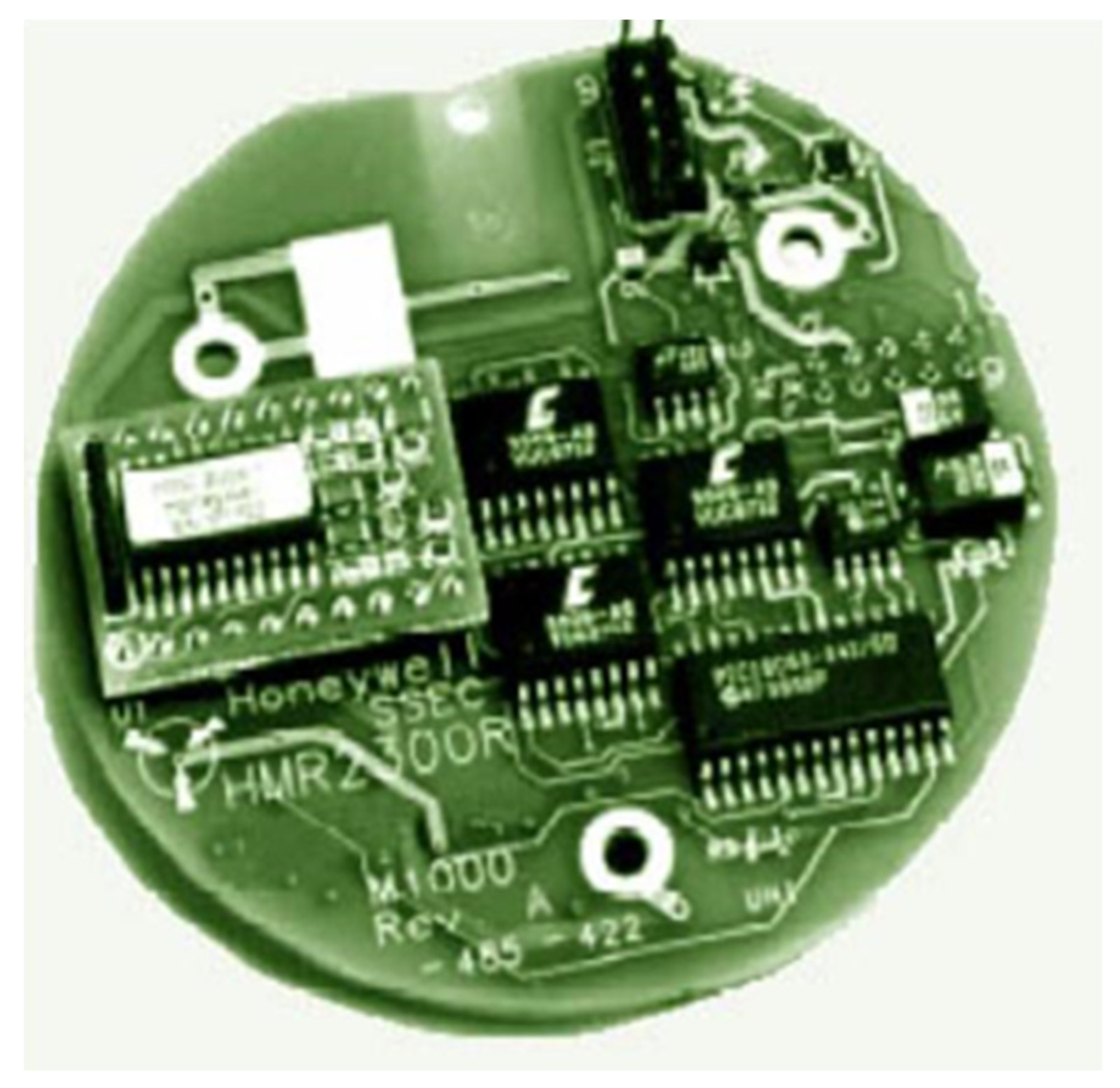
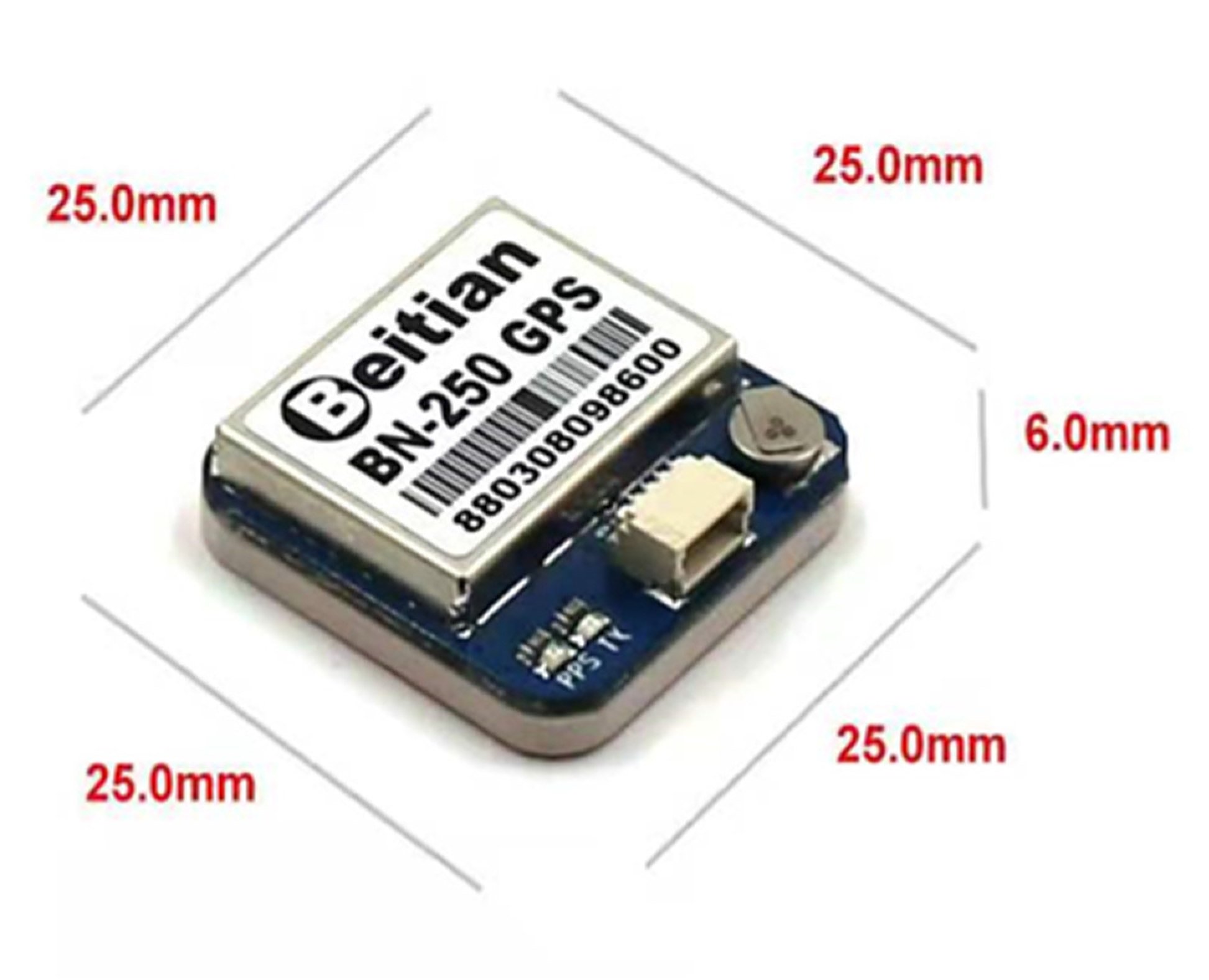
2.1. Principle of Measurement of Attitude Angle Information by the Magnetometer and Satellite System

The basic principle of using a magnetometer and satellite data to measure the attitude angle of a UAV is as follows. The three-axis magnetometer and UAV body are installed by strapdown inertial navigation, and the direction of the sensitive axis of the magnetometer is the same as that of the body coordinate system. During the flight, the magnetometer measures geomagnetic data in real-time. The relationship matrix between the magnetometer measurement data, geomagnetic data, and body attitude angle is:

$$\left[\begin{array}{c}{h}_{bx}\\ h_{by}\\ h_{bz}\end{array}\right]=\left[\begin{array}{ccc}\cos \theta \cos \psi & \cos \theta \sin \psi & -\sin \theta \\ -\cos \gamma \sin \psi +\sin \gamma \sin \theta \cos \psi & \cos \gamma \cos \psi +\sin \gamma \sin \theta \sin \psi & \sin \gamma \cos \theta \\ \sin \gamma \sin \psi +\cos \gamma \sin \theta \cos \psi & -\sin \gamma \cos \psi +\cos \gamma \sin \theta \sin \psi & \cos \gamma \cos \theta \end{array}\right]\left[\begin{array}{c}{h}_{nx}\\ h_{ny}\\ h_{nz}\end{array}\right]$$

(1)

where $h_{nx},h_{ny},h_{nz}$ are the geomagnetic components in the navigation coordinate system; $h_{bx},h_{by},h_{bz}$ are the projection components of the geomagnetic vector in the body coordinate system; and $\psi ,\theta ,\gamma$ are the yaw angle, pitch angle, and roll angle, respectively, in the navigation coordinate system.

According to Equation (1), the attitude angle of the body can be obtained using numerous feasible solutions, which cannot meet measurement requirements in engineering practice. Therefore, the fusion of satellite measurement data is required to measure the UAV attitude angle.

In the actual stable flight of a UAV, the angle of attack and angle of sideslip are both relatively small. Therefore, in the body coordinate and speed coordinate systems, the following relationship is satisfied:

$$\begin{array}{l}\theta \approx \alpha +{\theta }_v\\ \psi \approx \beta +{\psi }_v\end{array}$$

(2)

where $\alpha$ and $\beta$ are the angles of attack and sideslip, respectively, and ${\theta }_v$ and ${\psi }_v$are the pitch angle and sideslip angle of the body, respectively.

Satellite measurement equipment can measure the longitude, latitude, altitude, and speed of the position of a UAV in real-time. In the speed and navigation coordinate system, the pitch and sideslip angles of the body can be obtained using the speed information provided by the measuring equipment, as shown in the following equation:

$$\begin{array}{l}{\theta }_v=\arctan (v_z/\sqrt{v_x^2+v_y^2})\\ {\psi }_v=\arctan (v_y/v_x)\end{array}$$

(3)

where $v_x,v_y,v_z$ are the northward, eastward, and ground speed, respectively.

As the flight angle of attack is small, the pitch and sideslip angles of the body can be approximated as the measurement data of the pitch and yaw angles, respectively.

For low-spin application scenarios, when the yaw angle and pitch angle are known, the value of the roll angle can be uniquely determined using Equation (1):

$$\gamma =\arctan \left(\frac{n{h}_{by}-m{h}_{bz}}{m{h}_{by}+n{h}_{bz}}\right)$$

(4)

where:

$$\begin{array}{l}m=-\sin \psi h_{nx}+\cos \psi h_{ny}\\ n=\cos \psi \sin \theta h_{nx}+\sin \psi \sin \theta h_{ny}+\cos \theta h_{nz}\end{array}$$

2.2. Combined Measurement Error Model

In the combined measurement scheme of the magnetometer and satellite measurement system, the measurement of the pitch angle and yaw angle relies only on the data provided by the satellite measurement system, which is relatively simple. However, the measurement of the roll angle depends on the combination of the magnetometer and satellite measurement system. Hence, the data and measurement accuracy are affected more. To examine this, the roll-angle error model is established in this study.

The measurement method represented by Equation (4) is expressed in the following form:

$$\gamma =F(h_{by},h_{bz},h_{nx},h_{ny},\theta ,\psi )$$

(5)

In the roll angle measurement method represented by Equation (5), in addition to the measurement error of the sensor itself and random error, the main error is derived from the hypothesis of a small angle of attack. The pitch and sideslip angles of the body are considered to be equal to the pitch and yaw angles, respectively. In other words, the pitch and yaw angles used in this method have certain errors. Here, the small angle of attack error and measurement error increment are expressed in the following form:

$$\begin{array}{l}\delta \theta =\theta -{\theta }_v\\ \delta \psi =\psi -{\psi }_v\\ \delta h_{by}=h_{by}-h_{byv}\\ \delta h_{bz}=h_{bz}-h_{bzv}\end{array}$$

(6)

The roll angle error in Equation (5) can be expressed as:

$$\delta \gamma =\frac{\partial F}{\partial \psi }\partial \psi +\frac{\partial F}{\partial \theta }\partial \theta +\frac{\partial \delta F}{\partial \delta h_{by}}\partial h_{by}+\frac{\partial F}{\partial h_{bz}}\partial h_{bz}$$

(7)

where:

$$\frac{\partial F}{\partial \psi }=\frac{\frac{\partial n}{\partial \psi }m-\frac{\partial m}{\partial \psi }n}{a^2+b^2}$$

$$\frac{\partial m}{\partial \psi }=\cos \psi \sin \theta h_{ny}-\sin \psi \sin \theta h_{nx}$$

$$\frac{\partial n}{\partial \psi }=-\cos \psi h_{nx}-\sin \psi h_{ny}$$

$$\frac{\partial F}{\partial \theta }=\frac{\frac{\partial n}{\partial \theta }m-\frac{\partial m}{\partial \theta }n}{a^2+b^2}$$

$$\frac{\partial n}{\partial \theta }=\cos \psi \cos \theta h_{nx}+\sin \psi \cos \theta h_{ny}-\sin \theta h_{nz}$$

$$\frac{\partial m}{\partial \theta }=0$$

$$\frac{\partial F}{\partial h_{by}}=\frac{1}{1+w^2}\frac{n(v-u)}{v^2}$$

$$\frac{\partial F}{\partial h_{bz}}=\frac{1}{1+w^2}\frac{m(v-u)}{v^2}$$

$$u=n{h}_{by}-m{h}_{bz}$$

$$v=m{h}_{by}+n{h}_{bz}$$

$$w=\frac{u}{v}$$

2.3. Measurement Error Analysis

In Equation (7), the roll angle error depends on the $h_{by}$ and $h_{bz}$ errors, pitch angle $\theta$, yaw angle $\psi$, and incremental errors $\delta \theta$ and $\delta \psi$ measured by the magnetometer.

The measurement errors of the magnetometer mainly include the inconsistency of the sensitivity of each axis, zero drift of the measuring device, interference of external magnetic field sources, interference of internal circuits, the magnetization material of the application object (iron, chromium, nickel and its alloys), and occasional measurement errors and jump points.

The errors in the pitch angle $\theta$ and yaw angle $\psi$ mainly originate from the errors of the satellite measurement equipment, including system positioning errors caused by an insufficient number of satellites, external environment interference errors, and system jump points. There are various random errors in the measurement process of satellite positioning systems, which mainly include ephemeris error and satellite clock error related to the performance of the satellite itself; factors related to the propagation path such as stratospheric delay, ionospheric delay, and multiple path effects; receiver-related factors such as receiver antenna phase center deviation and change, receiver clock deviation, and signal delay deviation between different signal channels.

The errors in the pitch angle rate $\dot{\theta }$ and yaw angle rate $\dot{\psi }$ are high-frequency errors, and the incremental errors $\delta \theta$ and $\delta \psi$ of the pitch angle $\theta$ and yaw angle $\psi$ are algorithmic errors.

Generally, errors include the following: external or system interference (external magnetic field source interference, internal circuit interference, and magnetization influence), measurement error (high-frequency error, noise interference, jump points, etc.), system error (different axial sensitivity, zero drift, etc.), and algorithm errors (deviations caused by the assumption of a small angle of attack).

Different solutions must be adopted for different error characteristics to improve the accuracy of the system. Compensation algorithms can be used to compensate for external interference, electromagnetic and magnetization interference of the system itself, and other external or system interferences. These can be processed by filtering algorithms, and system errors can be corrected by data fitting. After processing by various methods, good measurement accuracy can be achieved to meet the needs of engineering practice. This study focuses on methods to eliminate external or system interference and measurement errors.

3. Magnetometer Calibration Based on Least-Squares Fitting Algorithm

In a certain region, the magnetic field of the Earth is uniform. If the three magnetic sensitive devices of the magnetometer are installed in three mutually perpendicular directions along the axis of the UAV body, after collecting sufficient data in each azimuth, the spatial distribution of these data should theoretically be such that the center of a sphere is at the origin of the coordinate sphere. However, owing to the influence of factors such as zero drift of the sensitive device and the different sensitivities of each axis, the originally collected data are neither at the center of the coordinate nor the sphere. To synchronize the measured data relative to the theoretical model, calibration of the original data is necessary. Generally, the calibration process includes two aspects: ellipsoid calibration and spherical calibration.

3.1. Ellipsoid Model

For magnetometers with three sensitive axes installed perpendicular to each other, the originally collected data represents a spatial ellipsoid that is roughly distributed along three axes parallel to the body axis. The aim of ellipsoid calibration is to use statistical methods to determine the ellipsoid equation with the smallest average variance of the collected data. In this study, we used the least-squares method to calibrate the magnetometer.

The general equation of the ellipsoid can be expressed as:

$$a_1{x}^2+a_2{y}^2+a_3{z}^2+a_{4}xy+a_{5}xz+a_{6}yz+a_{7}x+a_{8}y+a_{9}z=1$$

(8)

We write the standard equation in the following form:

$$1=(x^2\hspace{1em}{y}^2\hspace{1em}{z}^2\hspace{1em}xy\hspace{1em}xz\hspace{1em}yz\hspace{1em}xy\hspace{1em}z)\left(\begin{array}{c}{a}_1\\ ⋮\\ a_9\end{array}\right)$$

(9)

From a geometric perspective, the points distributed on the ellipsoid can be expressed in the following matrix form:

$$\begin{gathered} \left[\begin{array}{ccc}x-c_x& y-c_y& z-c_z\end{array}\right]{\left[\begin{array}{ccc}{r}_{11}& r_{12}& r_{13}\\ r_{21}& r_{22}& r_{23}\\ r_{31}& r_{32}& r_{33}\end{array}\right]}^T\left[\begin{array}{ccc}{\lambda }_1& 0& 0\\ 0& {\lambda }_2& 0\\ 0& 0& {\lambda }_3\end{array}\right]\left[\begin{array}{ccc}{r}_{11}& r_{12}& r_{13}\\ r_{21}& r_{22}& r_{23}\\ r_{31}& r_{32}& r_{33}\end{array}\right]\left[\begin{array}{c}x-c_x\\ y-c_y\\ z-c_z\end{array}\right] \\ =1+\left[\begin{array}{ccc}{c}_x& c_y& c_z\end{array}\right]{\left[\begin{array}{ccc}{r}_{11}& r_{12}& r_{13}\\ r_{21}& r_{22}& r_{23}\\ r_{31}& r_{32}& r_{33}\end{array}\right]}^T\left[\begin{array}{ccc}{\lambda }_1& 0& 0\\ 0& {\lambda }_2& 0\\ 0& 0& {\lambda }_3\end{array}\right]\left[\begin{array}{ccc}{r}_{11}& r_{12}& r_{13}\\ r_{21}& r_{22}& r_{23}\\ r_{31}& r_{32}& r_{33}\end{array}\right]\left[\begin{array}{c}{c}_x\\ c_y\\ c_z\end{array}\right] \end{gathered}$$

(10)

The above equation can be expressed as:

$$\begin{array}{cc}\left[X-C\right]M& \left[X-C\right]T=1+CM{C}^T\hfill \\ & XM{X}^T-2CM{X}^T+CM{C}^T=1+CM{C}^T\hfill \end{array}$$

(11)

where:

$X=\left[\begin{array}{ccc}x& y& z\end{array}\right]$ represents a point on the ellipsoid and $C=\left[\begin{array}{ccc}{c}_x& c_y& c_z\end{array}\right]$ is the coordinate of the center of the ellipsoid.

$$M=R^{T}BR={\left[\begin{array}{ccc}{r}_{11}& r_{12}& r_{13}\\ r_{21}& r_{22}& r_{23}\\ r_{31}& r_{32}& r_{33}\end{array}\right]}^T\left[\begin{array}{ccc}{\lambda }_1& 0& 0\\ 0& {\lambda }_2& 0\\ 0& 0& {\lambda }_3\end{array}\right]\left[\begin{array}{ccc}{r}_{11}& r_{12}& r_{13}\\ r_{21}& r_{22}& r_{23}\\ r_{31}& r_{32}& r_{33}\end{array}\right]=\left[\begin{array}{ccc}{a}_1& a_4/2& a_5/2\\ a_4/2& a_2& a_6/2\\ a_5/2& a_6/2& a_3\end{array}\right]$$

According to the ellipsoid model, the following ellipsoid parameters can be obtained:

Sphere center coordinates:

$$C=0.5\left[\begin{array}{ccc}{a}_7& a_8& a_9\end{array}\right]M^{-1}$$

$$\begin{array}{c}\mathrm{X}-\mathrm{axis}\mathrm{length}:x_{scale}=\sqrt{\frac{SS}{{\lambda }_1}}\\ \mathrm{Y}-\mathrm{axis}\mathrm{length}:y_{scale}=\sqrt{\frac{SS}{{\lambda }_2}}\\ \mathrm{Z}-\mathrm{axis}\mathrm{length}:z_{scale}=\sqrt{\frac{SS}{{\lambda }_3}}\end{array}$$

where: $SS=CM{C}^T+1$

3.2. Ellipsoid Fitting Based on Least Squares Algorithm

If n sets of data are collected by the magnetometer, the ellipsoid equation can be expressed as:

$$\left[\begin{array}{c}1\\ 1\\ ⋮\\ 1\end{array}\right]=\left[\begin{array}{ccccccc}{x}_1^2& y_1^2& z_1^2& \cdots & x_1& y_1& z_1\\ x_2^2& y_2^2& z_2^2& \cdots & x_2& y_2& z_1\\ ⋮& ⋮& ⋮& \ddots & ⋮& ⋮& ⋮\\ x_n^2& y_n^2& z_n^2& \cdots & x_n& y_n& z_n\end{array}\right]\left[\begin{array}{c}{a}_1\\ a_2\\ ⋮\\ a_9\end{array}\right]\mathbf{}$$

(12)

We write,

$$H=\left[\begin{array}{ccccccc}{x}_1^2& y_1^2& z_1^2& \cdots & x_1& y_1& z_1\\ x_2^2& y_2^2& z_2^2& \cdots & x_2& y_2& z_1\\ ⋮& ⋮& ⋮& \ddots & ⋮& ⋮& ⋮\\ x_n^2& y_n^2& z_n^2& \cdots & x_n& y_n& z_n\end{array}\right]\mathbf{}$$

$$k={\left[\begin{array}{cccc}{a}_1& a_2& \cdots & a_9\end{array}\right]}^T\mathbf{}$$

Ellipsoid fitting determines a set of ellipsoid parameter values K, with the smallest variance based on the original measurement data and equation. According to the least squares algorithm, the ellipsoid parameters that lead to the smallest measurement error are:

$$k={(H^{T}H)}^{-1}{H}^T$$

(13)

3.3. Magnetometer Calibration

The ellipsoid parameters obtained by fitting are used to calibrate the data measured by the magnetometer. First, we calibrate the origin of the ellipsoid coordinates as:

$$h_{bt}=h_b-C$$

(14)

After this correction, the measurement data are distributed in an ellipsoid with the coordinate origin as the center of the sphere, which also eliminates the zero-point error.

Simultaneously, to eliminate the difference in the sensitivity of each axis, spherical calibration is required. When performing spherical calibration, a reference axis must be determined first. In the magnetometer-satellite measurement of the UAV attitude angle, the Y-axis is more important. Therefore, the Y-axis can be selected as the reference for spherical correction, namely:

$$h_b=y_{scale}*h_{bt}.*[\begin{array}{ccc}{x}_{scale}& y_{scale}& z_{scale}\end{array}]$$

(15)

4. Interference Compensation Algorithm

4.1. Principle of Interference Compensation

Considering interference conditions such as external magnetic field interference, carrier residual magnetic field, and magnetizing magnetic field interference, the measurement model of the magnetometer can be expressed as:

$$B_m=C{B}_e^r+B_p+K_{i}C{B}_e^r=(I_{3\times 3}+K_i)C{B}_e^r+B_p$$

(16)

where $B_m$ is the value measured by the magnetometer; and $C$ is the conversion matrix from the reference coordinate system to the carrier coordinate system. The reference coordinate system is fixed and can be flexibly defined according to the actual trajectory; $B_e^r$ is the local geomagnetic vector field, which can generally be regarded as a fixed vector field; $B_p$ is the external magnetic field interference and carrier remnant magnetic field; and $K_i$ is the magnetic susceptibility matrix.

The formal transformation of Equation (8) can be obtained as:

$$B_m-(I_{3\times 3}+K_i)C{B}_e^r-B_p=0$$

(17)

Let, $K={\left(I_{3\times 3}+K_i\right)}^{-1}$ and $B_{pk}=K{B}_P$. Equation (9) can be expressed as:

$$K{B}_m-C{B}_e^r-B_{pk}=0$$

(18)

From Equation (10), the following linear homogeneous equations is obtained:

$$AX=0_{N\times 1}$$

(19)

where:

$$A=\left[\begin{array}{ccc}-C_1& B_{m,1}^T\otimes I_{3\times 3}& -I_{3\times 3}\\ -C_2& B_{m,2}^T\otimes I_{3\times 3}& -I_{3\times 3}\\ ⋮& ⋮& ⋮\\ -C_N& B_{m,N}^T\otimes I_{3\times 3}& -I_{3\times 3}\end{array}\right],X=\left[\begin{array}{c}{B}_e^r\\ vec(K^T)\\ B_{pk}\end{array}\right]$$

$\otimes$ is the Kronecker product, and $vec$ represents a matrix algorithm, i.e., a new matrix is formed by stacking the columns of the matrix in order from top to bottom; N is the data obtained by N groups of measurements.

Generally, the total strength of the geomagnetic field is constant and known throughout the entire flight range. Thus, the following equation is obtained:

$$X^{T}DX={\left|B_e^r\right|}^2$$

(20)

where:

$$D=\left[\begin{array}{cc}{I}_{3\times 3}& 0_{3\times 12}\\ 0_{12\times 3}& 0_{12\times 12}\end{array}\right]$$

The solution of the linear homogeneous equations determined by Equation (11) can be transformed into an optimization problem to obtain the minimum X value of the objective function $f\left(X\right)=X^T{A}^{T}AX$ under the constraints of Equation (12).

The Lagrangian multiplier method is used to solve this optimization problem. The Lagrangian function is defined as:

$$L(X,\lambda )=X^T{A}^{T}AX+\lambda (X^{T}DX-{\left|B_e^r\right|}^2)$$

(21)

Additionally:

$$\begin{array}{l}\partial L/\partial X=0\\ \partial L/\partial \lambda =0\end{array}$$

(22)

$$\begin{array}{l}{A}^{T}AX=\lambda DX\\ X^{T}DX={\left|B_e^T\right|}^2\end{array}$$

(23)

As $\lambda$ is the generalized characteristic root of matrices $A^{T}A$ and $D$, and $X$ is the eigenvector family corresponding to the characteristic root, we obtain:

$$X^T{A}^{T}AX=\lambda {\left|B_e^T\right|}^2$$

(24)

Therefore, when $\lambda$ assumes the minimum value ${\lambda }_{min}$ in the generalized characteristic root, the value of $f\left(x\right)$ is the smallest. The feature vector family corresponding to $X$ and ${\lambda }_{min}$ can be expressed as:

$$X=\omega v$$

(25)

where A is the coefficient to be determined, and B is the eigenvector corresponding to the generalized eigenvalue. Incorporating Equation (25) into Equation (20), we obtain:

$$\omega =\pm \sqrt{{\left|B_e^r\right|}^2/(v^{T}Dv)}$$

(26)

4.2. Coefficient Tuning Independent of Environmental Information

Section 4.1 presents the magnetometer compensation method under the interference conditions of the external magnetic field, carrier residual magnetic field, magnetizing magnetic field, and others. However, regarding the final result, Equation (18) cannot uniquely determine the compensation coefficient. Therefore, it is necessary to determine the compensation coefficient separately.

If the geographic coordinate system is selected as the reference coordinate system, the north component of the geomagnetic vector is generally positive, i.e., the north component of $B_e^r$ is positive.

$$B_e^r(1)>0$$

(27)

From Equations (19), (25) and (27), we obtain:

$$\omega v(1)=X(1)>0$$

(28)

From Equation (28), the value of the compensation coefficient can be uniquely determined.

This method can determine the compensation coefficient, but also has limitations. The geographic coordinate system must be selected as the reference coordinate system. Even if this restriction is relaxed, it is necessary to clearly determine the position of the selected reference coordinates relative to the geographic coordinate system. This is inconvenient for practical application. Next, we introduce a compensation coefficient tuning method that does not depend on environmental information.

By using the information of the carrier itself to adjust the compensation coefficient, we can avoid dependence on environmental information. In actual application scenarios of magnetometers, the UAV body generally avoids the use of magnetized materials up to the maximum possible extent. Therefore, the absolute value of each element of matrix $k_i$ is significantly less than 1, such that the main diagonal elements of matrix $\left(I_{3\times 3}+K_i\right)$ are greater than 0. From Equations (19) and (25), we obtain:

$$\begin{array}{l}K=\left[\begin{array}{ccc}X(4)& X(5)& X(6)\\ X(7)& X(8)& X(9)\\ X(10)& X(11)& X(12)\end{array}\right]\\ =\omega \left[\begin{array}{ccc}v(4)& v(5)& v(6)\\ v(7)& v(8)& v(9)\\ v(10)& v(11)& v(12)\end{array}\right]\end{array}$$

(29)

According to the definition of $K$:

$$I_{3\times 3}+K_i=K^{-1}=\frac{1}{\omega }{\left[\begin{array}{ccc}v(4)& v(5)& v(6)\\ v(7)& v(8)& v(9)\\ v(10)& v(11)& v(12)\end{array}\right]}^{-1}$$

(30)

It is evident from Equation (30) that the value of $\mathsf{\omega }$ is the value of all elements (greater than 0) on the main diagonal of the matrix $K^{-1}$. After calculating $\mathsf{\omega }$, we obtain:

$$B_{pk}=\omega \left[\begin{array}{c}v(13)\\ v(14)\\ v(15)\end{array}\right]$$

(31)

The final compensation result can be written as:

$$\begin{array}{l}{K}_i=K^{-1}-I_{3\times 3}\\ B_p=K^{-1}{B}_{pk}\end{array}$$

(32)

From Equations (16), (29), (31) and (32), the geomagnetic vector in the reference frame after compensation can be obtained as:

$$B_m=C{B}_e^r+B_p+K_{i}C{B}_e^r=(I_{3\times 3}+K_i)C{B}_e^r+B_p$$

(33)

5. Measurement Error Compensation Based on Kalman Filter Algorithm

5.1. “Current” Statistical Motion Model

To eliminate the measurement error of the magnetometer and satellite positioning system, the Kalman filter algorithm is used. The Kalman filter is an effective method of handling measurement errors of dynamic system data, which can considerably improve the accuracy of dynamic measurements. Therefore, Kalman filter technology has been widely used in dynamic positioning.

In the method of combining a magnetometer and satellite positioning to measure attitude data, the state equation of the sensor is continuous, but the measurement equation is discrete. In other words, the measurement information of the sensor is obtained by sampling from the state equation of the sensor in a certain time interval. Therefore, after eliminating the measurement error, a continuous-discrete system model must be established.

According to the actual characteristics of the combined attitude measurement of the magnetometer and satellite positioning system, a continuous state model of the following form is established:

$$\left[\begin{array}{c}\dot{x}(t)\\ \ddot{x}(t)\\ \stackrel{⃛}{x}(t)\end{array}\right]=\left[\begin{array}{ccc}0& 1& 0\\ 0& 0& 1\\ 0& 0& -N\end{array}\right]\left[\begin{array}{c}x(t)\\ \dot{x}(t)\\ \ddot{x}(t)\end{array}\right]+\left[\begin{array}{c}0\\ 0\\ 1\end{array}\right]\varpi (t)$$

(34)

where $x$ is the state quantity, which is the spatial position of the satellite measurement system. For the magnetometer, it is the change equation of the local geomagnetic intensity in each axis. $N$ is the rate of change of each state, and $\overline{\omega }$ represents various interference noises for each state.

Equation (34) presents greater difficulties in practical applications. First, the carrier does not move at a standard constant velocity or with constant acceleration, and there is a certain model error. In addition, the magnetic intensity model of each axis must rely on the shooting direction and attitude data of the missile, which are difficult to obtain quickly and accurately. Therefore, there are several limitations in the practical engineering application of the motion model of Equation (34).

In order to solve this problem, in this study, we use the “current” statistical model to optimize the motion model. When a state changes at a certain rate, the change in the rate value at the next moment should be limited, and can only be within the neighborhood of the current value. The “current” statistical model describes the changes in the current probability density of a state with an appropriate function distribution, and its mean value is the predicted value of the “current” rate. The random rate change can also satisfy the first-order time correlation characteristics on the time axis. The “current” statistical model is essentially a non-zero mean time-dependent model.

Based on the “current” statistical model, we can write:

$$\ddot{x}(t)=\tilde{\varpi }(t)+\varpi (t)$$

(35)

$$\dot{\varpi }(t)=-N\varpi (t)+\omega (t)$$

(36)

where $\tilde{\overline{\omega }}\left(t\right)$ is the “current” average value of the rate of change, which can be regarded as constant within the same sampling period of the sensor.

Hence,

$${\varpi }_1(t)=\tilde{\varpi }(t)+\varpi (t)=\ddot{x}(t)$$

(37)

$${\dot{\varpi }}_1(t)=\dot{\tilde{\varpi }}(t)+\dot{\varpi }(t)$$

(38)

In the same sampling period, we can consider that $\dot{\tilde{\overline{\omega }}}\left(t\right)=0$. Then, $\dot{{\varpi }_1}\left(t\right)=\dot{\varpi }\left(t\right)$. $\varpi \left(\mathrm{t}\right)={\varpi }_1\left(\mathrm{t}\right)-\dot{\tilde{\varpi }}\left(\mathrm{t}\right)$ can be obtained from Equation (29), and FFF can be obtained by substituting this equation and Equation (28) into $\dot{{\varpi }_1}\left(t\right)=\dot{\varpi }\left(t\right)$.

$${\dot{\varpi }}_1(t)=-N{\varpi }_1(t)+N\tilde{\varpi }(t)+\omega (t)$$

(39)

which is expressed as:

$$\stackrel{⃛}{x}(t)=-N\ddot{x}(t)+N\tilde{\varpi }(t)+\omega (t)$$

(40)

This is the state equation, which is the “current” statistical model of mobile carriers. At this time, Equation (34) is expressed as:

$$\begin{array}{l}\left[\begin{array}{c}\dot{x}(t)\\ \ddot{x}(t)\\ \stackrel{⃛}{x}(t)\end{array}\right]=\left[\begin{array}{ccc}0& 1& 0\\ 0& 0& 1\\ 0& 0& -N\end{array}\right]\left[\begin{array}{c}x(t)\\ \dot{x}(t)\\ \ddot{x}(t)\end{array}\right]+\left[\begin{array}{c}0\\ 0\\ 1\end{array}\right]\tilde{\varpi }(t)+\left[\begin{array}{c}0\\ 0\\ 1\end{array}\right]\omega (t)\\ =\left[\begin{array}{ccc}0& 1& 0\\ 0& 0& 1\\ 0& 0& -N\end{array}\right]\left[\begin{array}{c}x(t)\\ \dot{x}(t)\\ \ddot{x}(t)\end{array}\right]+\left[\begin{array}{c}0\\ 0\\ 1\end{array}\right](\tilde{\varpi }(t)+\omega (t))\end{array}$$

(41)

5.2. Continuous-Discrete System Kalman Filter Algorithm

According to Equation (33), the system equation and measurement equation are described in the following form:

$$\dot{X}(t)=F(t)X(t)+G(t)W(t)$$

(42)

$$Z_k=H_k{X}_k+V_K$$

(43)

The continuous-discrete system Kalman filter equation is expressed as follows. The time correction equation is:

$$\dot{\widehat{X}}(t)=F(t)\widehat{X}(t)$$

(44)

$$\dot{P}(t)=F(t)P(t)+P(t)F^T(t)+G(t)Q(t)Q^T(t)$$

(45)

Here, $t_{k-1}\le t\le t_k$.

The measurement correction equation is:

$${\dot{\widehat{X}}}_k={\widehat{X}}_{k,k-1}+K_k[Z_k-H_k{\widehat{X}}_{k,k-1}]$$

(46)

$$K_k=P_{k,k-1}{H}_k^T{(H_k{P}_{k,k-1}{H}_k^T+R_k)}^{-1}$$

(47)

$$P_{k,k-1}={\varphi }_{k,k-1}{P}_{k-1}{\varphi }_{k,k-1}^T+{\Gamma }_{k-1}{Q}_{k-1}{\Gamma }_{k-1}^T$$

(48)

$$P_k=P_{k,k-1}-K_k{H}_k{P}_{k,k-1}$$

(49)

6. Test and Analysis

In order to verify the validity of the algorithm, a laboratory test method is used, and the test equipment is a three-axis turntable, as shown in Figure 1. Here, the HMR2300R three-axis strapdown magnetometer and BN-250 positioning + antenna integrated module of the Honeywell company are selected as the test equipment. The equipment is shown in Figure 2 and Figure 3.

In order to verify the validity of the algorithm, a laboratory test method is used, and the test equipment is a three-axis turntable, as shown in Figure 1. Here, the HMR2300R three-axis strapdown magnetometer and BN-250 positioning + antenna integrated module of the Honeywell company are selected as the test equipment. The equipment is shown in Figure 2 and Figure 3.

The experimental steps are as follows:

• Step 1: Connect the direction of the sensor to the turntable and make it consistent;
• Step 2: Fix the pointing angle of the turntable;
• Step 3: Adjust the pitch angle of the turntable to be fixed, so that the turntable rolls and records the data;
• Step 4: Adjust the pitch of the turntable to another angle and fix it to make the turntable roll and record data; repeat this step to collect data at different pitch angles;
• Step 5: Fix the pitch angle of the turntable;
• Step 6: Adjust the pointing angle of the turntable to be fixed, so that the turntable rolls and records the data;
• Step 7: Adjust the pointing of the turntable to another angle and fix it, so that the turntable rolls and records data; repeat this step to collect data at different pointing angles;

The test location and local geomagnetic information are shown in

Table 1. Local magnetic field information.

Latitude:	31.8597691°
Longitude:	117.2710962°
Height:	273.00 m
Total field:	42965 nT
Magnetic declination:	−4.932°
Magnetic inclination:	48.453°
X component:	28391 nT
Y component:	−2450 nT
Z component:	32155 nT
Horizontal component:	28496 nT

.

To verify the compensation algorithm, five 10 mm neodymium iron boron high-strength magnets were placed 0.3 m in the horizontal direction on the left side of the turntable.

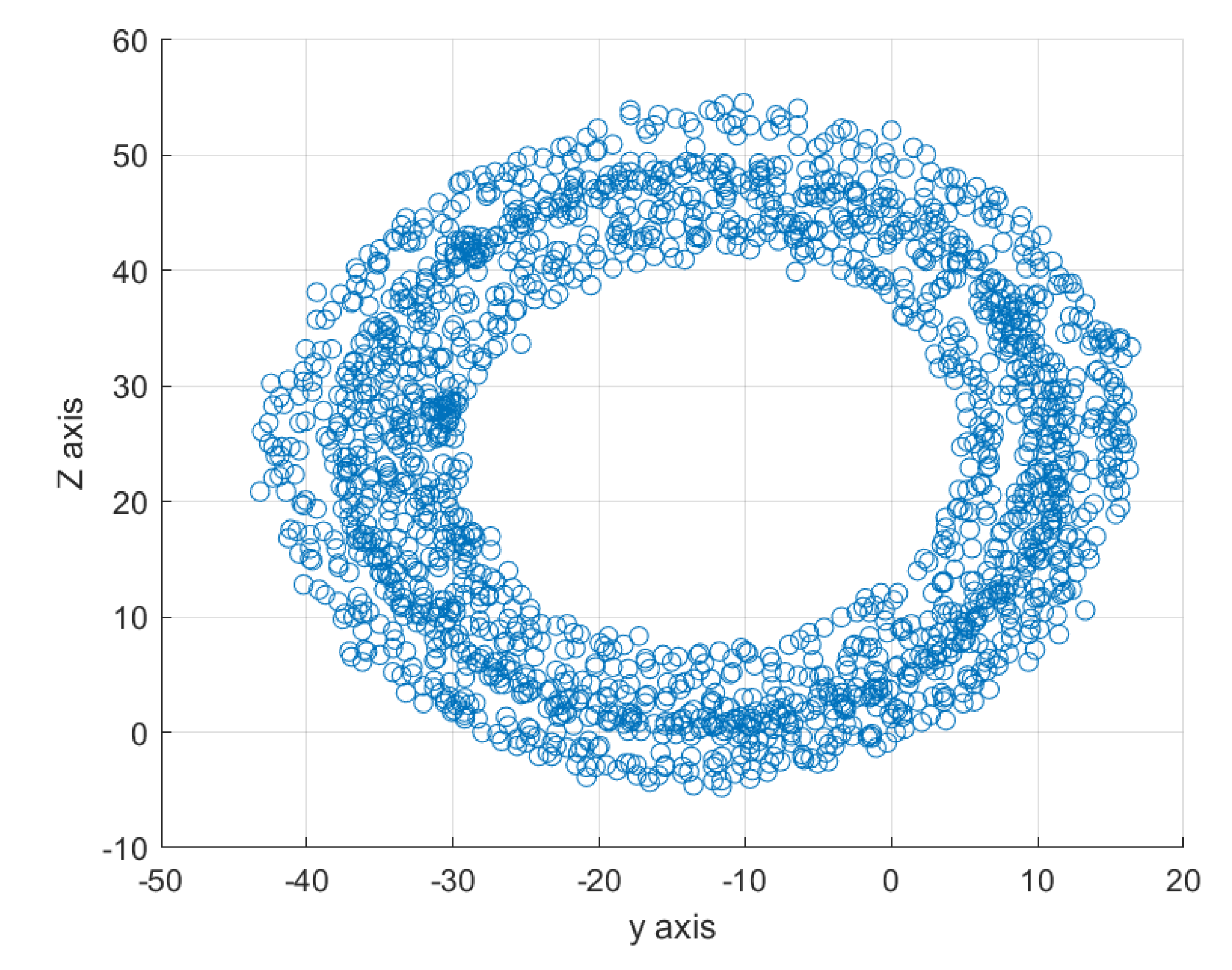
6.1. Magnetometer Calibration

The magnetometer was strapped in the axial direction of the three-axis turntable and collected 4250 sets of data. The initial distribution of the data is shown in Figure 4, Figure 5 and Figure 6.

From the distribution of the initial measurement data, it can be observed that the three axes of the magnetometer deviate from the theoretical value, and the measurement sensitivity of the three axes is not consistent.

Using the least-squares fitting algorithm, the results of the fitting and calibration of the magnetometer are as follows. For the ellipsoid equation represented by Equation (7), the fitting coefficients are:

a1 = 1/2565.8112; a2=1.8376/2565.8112; a3 = 1.8774/2565.8112; a4 = a5 = a6 = 0; a7 = 101.1578/2565.8112; a8 = 47.3103/2565.8112; a9 = −93.6223/2565.8112

The coordinates of the center of the ellipsoid are: $\left[\begin{array}{ccc}-50.5790& -12.8727& 24.9344\end{array}\right]$

The x−axis radius is: 38.2640

The y−axis radius is: 28.2269

The z−axis radius is: 27.9265

Using the aforementioned calibration method, the data distribution after the calibration of the magnetometer is shown in Figure 7.

As shown in Figure 4, the spatial distribution of the magnetometer measurement data after calibration is spherical, which is consistent with the theoretical spatial distribution.

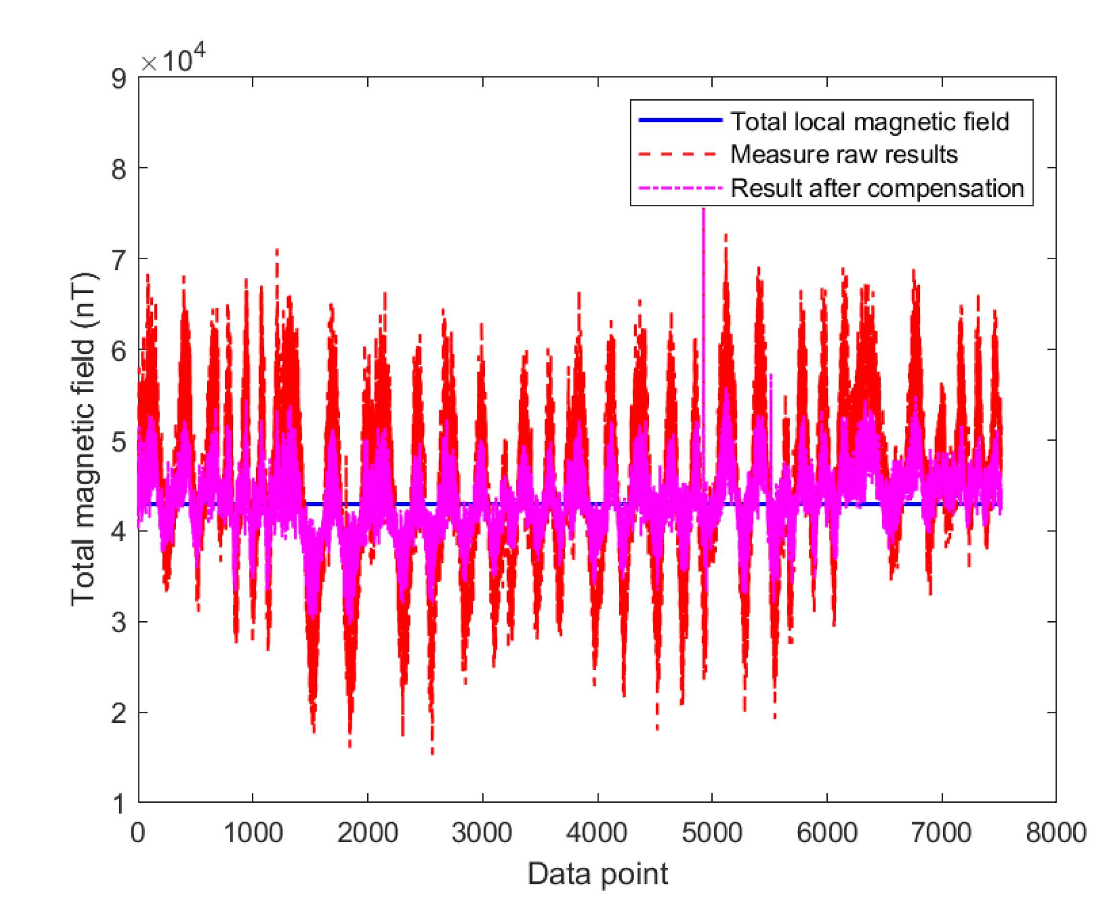
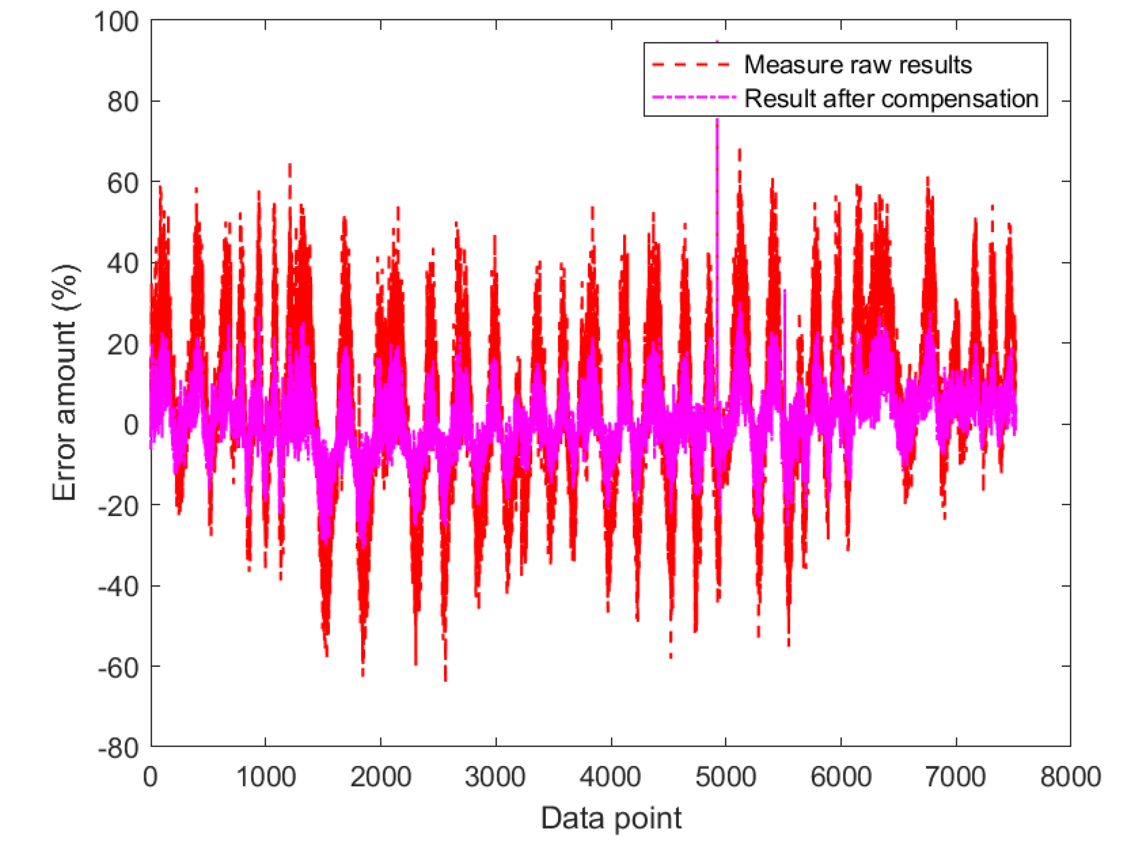
6.2. Compensation Algorithm Verification

According to the compensation methods and steps presented in this article, the following compensation results are calculated:

$$K_i=\left[\begin{array}{ccc}-0.0251& 0.0113& -0.0087\\ -0.0384& 0.3031& 0.0034\\ 0.093& -0.0074& -0.0059\end{array}\right]B_p={\left[\begin{array}{ccc}34.2870& 746.2563& 67.3204\end{array}\right]}^T$$

The measurement result of a single axis changes with change in the attitude angle of the carrier. Therefore, the measurement data of a single axis lacks standard comparison data. To solve this problem, we have used the total magnetic intensity to perform an algorithmic effect analysis. The relationship between the three axial magnetic field strengths and total magnetic field strength is:

$$H_b=\sqrt{h_{bx}^2+h_{by}^2+h_{bz}^2}$$

The local magnetic field strength, original measurement data, and compensated data are shown in Figure 8 and Figure 9, respectively.

From the analysis of the data in Figure 8, after using the compensation algorithm, the deviation of the data is considerably reduced compared to the local magnetic field, and the fluctuation of the data is smaller. As shown in Figure 9, the measurement data error is significantly reduced after compensation. After further analysis, it can be observed that the average absolute error of the original measurement data compared to the local magnetic field strength is 17.80%, and the average absolute error of the measurement data compensated by the compensation algorithm is 6.86% compared to the local magnetic field strength. From the data, error distribution, and absolute error analysis results, after using the compensation algorithm, the absolute measurement error of the magnetometer is reduced by 61.49%, which effectively compensates for external or system interference.

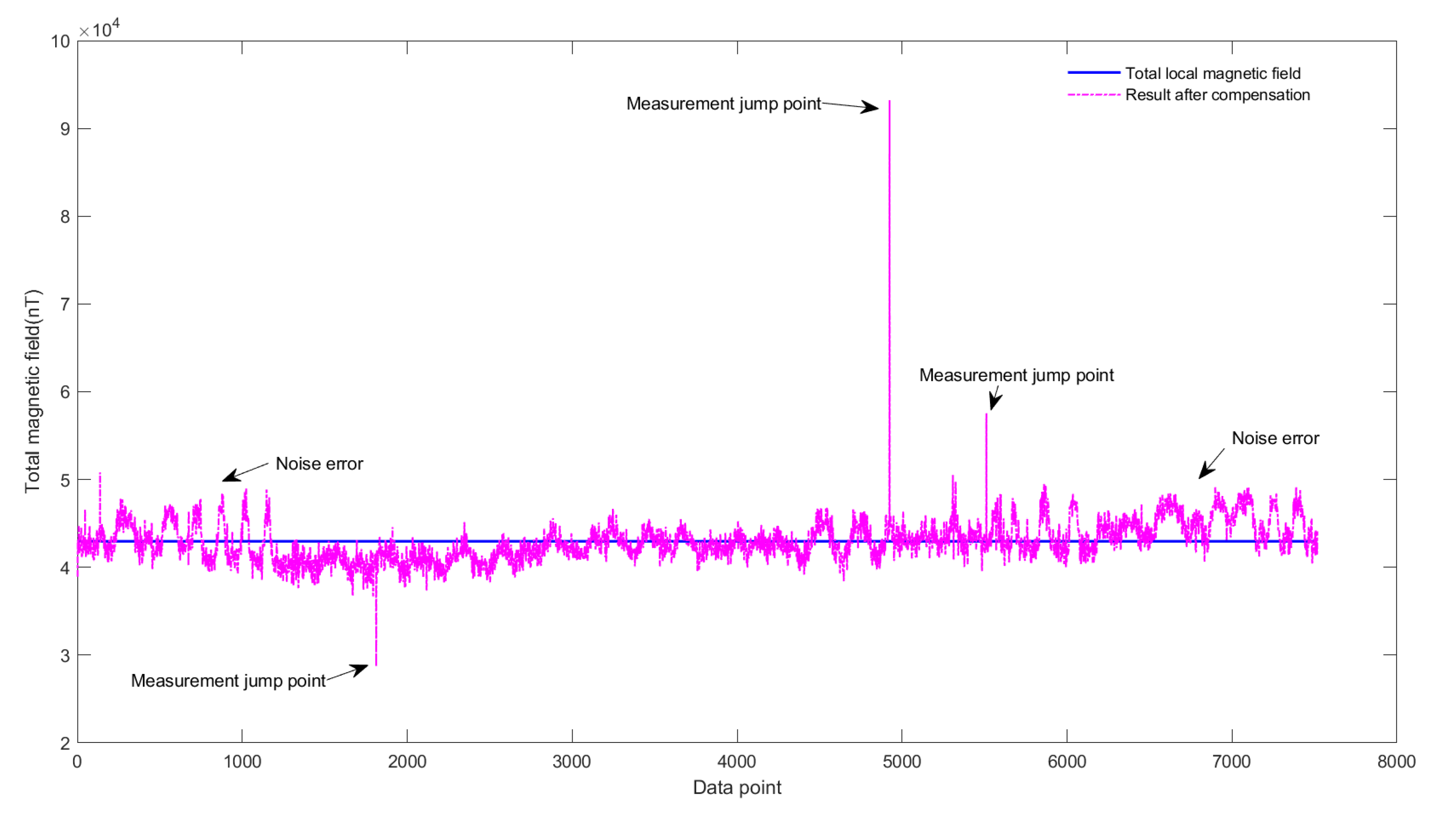
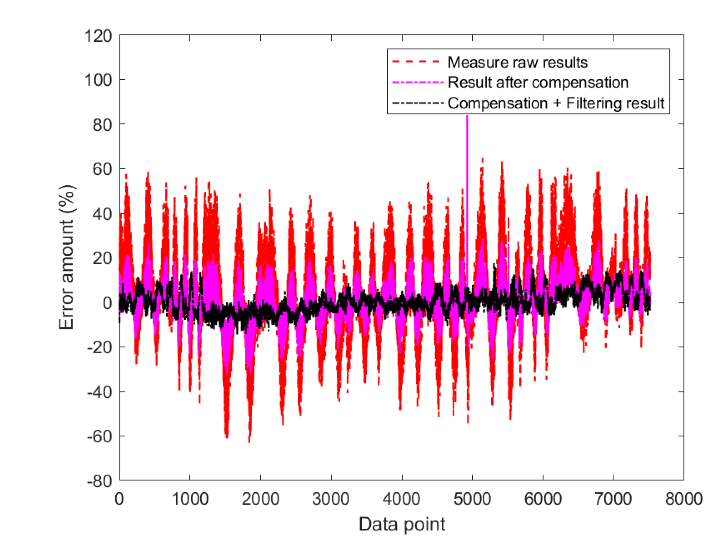
6.3. Kalman Filter Algorithm

The measurement accuracy can be improved significantly after external or system interference is compensated. However, the compensated data are still influenced by measurement jump points and noise errors. As shown in Figure 10, in the 7500 sets of measurement data, there are four obvious jump points. Such incorrect measurement jump points can cause hidden dangers to the safe flight of UAVs. At the same time, in Figure 10, there is a greater influence of noise at the beginning and end of the measurement, which reduces the measurement accuracy of the attitude angle.

Using the continuous-discrete model established in this study, the measurement equation step size adopts the sampling period of the sensor, and the error model adopts the uncorrelated white Gaussian noise model. The measurement results and error comparisons before and after filtering are shown in Figure 11 and Figure 12.

From the analysis of the data in Figure 11, it can be observed that after applying the filtering algorithm, the deviation of the data is further reduced compared with the compensated magnetic field data. Additionally, the data fluctuation is weaker, and the impact of jumping points is eliminated. As shown in Figure 12, the measurement data error is further reduced after filtering. The analysis shows that compared to the 6.86% average absolute error of the local magnetic field strength, the measurement data compensated by the compensation algorithm is 3.95% of the average absolute error of the local magnetic field strength. From the data and error distribution, the absolute error analysis result shows that the absolute measurement error of the magnetometer is further reduced by 42.36% compared with the compensated data after filtering. This effectively eliminates the errors caused by jump points and noise.

7. Conclusions

In this study, we focus on the problems of external interference and measurement errors in the measurement of the UAV attitude angle. A combined measurement model is established based on the magnetometer-satellite positioning system combined with the measurement attitude angle program. According to the model, the source of the measurement error is analyzed, and the effects of external or system interference, measurement error, system error, and algorithm error on the final measurement error are clarified. The magnetometer has been tested and calibrated according to the ellipsoid fitting principle of the least squares method. To analyze the characteristics of measurement error factors, we have designed a compensation algorithm that does not depend on environmental information of the influence of external or system interference, which reduces the absolute measurement error of the magnetometer by 61.49% and effectively compensates for external or system interference. The continuous-discrete Kalman filter algorithm of the “current” model is established to reduce the measurement error such that the absolute measurement error of the magnetometer is further reduced by 42.36% relative to the compensated data, which effectively eliminates the error caused by jumping points and noise.

The experimental results show that the combined attitude angle measurement scheme of the magnetometer-satellite positioning system can improve measurement accuracy by effectively compensating for interference and by reducing jumping points or noise error. This proves the feasibility and effectiveness of the scheme, its suitability for UAV attitude angle measurement, and its high engineering application value.

References

1. Sun, Y.L.; Jiang, X. MEMS/Geomagnetism-based adaptive estimation algorithm of UAV heading and attitude. Sens. Microsyst. 2020, 39, 122–125. [Google Scholar]
2. Ji, H.D.; Jiang, W.G. Simulation research on attitude calculation based on multi-MEMS sensor combination. Instrum. Technol. Sens. 2020, 08, 85–89. [Google Scholar]
3. Liu, X.H.; Liu, X.X. UAV attitude calculation algorithm based on acceleration correction model. J. Northwest. Polytech. Univ. 2021, 39, 175–181. [Google Scholar] [CrossRef]
4. Xu, T.T.; Zhao, B.X.; Luo, Y.Z. Attitude data fusion algorithm of MEMS sensor components based on complementary-particle filter. Ordnance Ind. Autom. 2021, 40, 29–32. [Google Scholar]
5. Yu, C.Y.; Zhang, Z. Spherical robot attitude calculation based on complementary filtering and particle filter fusion. Robot. J. 2021, 43, 340–349. [Google Scholar]
6. An, L.L.; Wang, L.M.; Zhong, Y. A low-cost method for measuring speed and roll angle with a single-axis magnetic sensor. Ordnance Equip. Eng. J. 2020, 41, 1–4. [Google Scholar]
7. Shao, W.P.; Sun, L.; Zhang, J.Y. A method for calculating the attitude of a rotating body based on a geomagnetic sensor. Sichuan Armamentary Eng. J. 2020, 41, 62–66. [Google Scholar]
8. Miao, J.S.; Zhai, Y.C.; Gou, Q.X. Calculation method of missile rolling attitude based on satellite/geomagnetic combination. J. Missile Guid. 2014, 34, 63–66. [Google Scholar]
9. Wu, Y.; Zou, D.; Liu, P. Dynamic Magnetometer Calibration and Alignment to Inertial Sensors by Kalman Filtering. IEEE Trans. Control. Syst. Technol. 2018, 26, 716–723. [Google Scholar] [CrossRef] [Green Version]
10. Wu, Y.; Zhu, M.; Yu, W. An Efficient Method for Gyroscope-aided Full Magnetometer Calibration. IEEE Sens. J. 2019, 19, 6355–6361. [Google Scholar]
11. Gao, L.Z.; Zhang, Y.Y.; Zhang, X.M. Fast calibration algorithm of installation angle for geomagnetic vector information measurement. Ordnance Equip. Eng. J. 2020, 4, 220–224. [Google Scholar]
12. Cao, P.; Yu, J.Y.; Wang, X.M. Research on high-frequency measurement and system error calculation of high-rotation projectile roll angle based on the combination of geomagnetism and satellite. Acta Armamentari 2014, 35, 795–800. [Google Scholar]
13. Liu, J.H.; Li, X.H. A universal vector compensation method for carrier interference in magnetometers. Chin. J. Sci. Instrum. 2020, 41, 112–118. [Google Scholar]
14. Rigatos, G.; Busawon, K.; Pomares, J. Nonlinear optimal control for a spherical rolling robot. Int. J. Intell. Robot. Appl. 2019, 3, 221–237. [Google Scholar] [CrossRef]
15. Indiveri, G.; Malerba, A. Complementary control for robots with actuator redundancy: An underwater vehicle application. Robot. Int. J. Inf. Educ. Res. Robot. Artif. Intell. 2017, 35, 206–223. [Google Scholar] [CrossRef]
16. Hu, Z.; Gallacher, B. Extended Kalman filtering based parameter estimation and drift compensation for a MEMS rate integrating gyroscope. Sens. Actuators A. Phys. 2016, 250, 96–105. [Google Scholar] [CrossRef] [Green Version]
17. Sabet, M.T.; Daniali, H.M.; Fathi, A.; Alizadeh, E. A Low-Cost Dead Reckoning Navigation System for an AUV Using a Robust AHRS: Design and Experimental Analysis. IEEE J. Ocean. Eng. 2017, 43, 927–939. [Google Scholar] [CrossRef]
Figure 1. Three-axis turntable.
Applsci 12 05947 g001
Figure 2. HMR2300R three axis strapdown magnetometer and carrier plate.
Applsci 12 05947 g002
Figure 3. BN-250 positioning + antenna integrated module.
Applsci 12 05947 g003
Figure 4. Spatial distribution of initial measurement data.
Applsci 12 05947 g004
Figure 5. X−Y plane distribution of initial measurement data.
Applsci 12 05947 g005
Figure 6. Y−Z plane distribution of initial measurement data.
Applsci 12 05947 g006
Figure 7. Spatial distribution of data after calibration.
Applsci 12 05947 g007
Figure 8. Compensation algorithm effect.
Applsci 12 05947 g008
Figure 9. Data error before and after compensation.
Applsci 12 05947 g009
Figure 10. The influence of jumps and noise.
Applsci 12 05947 g010
Figure 11. Data comparison before and after filtering.
Applsci 12 05947 g011
Figure 12. Data error before and after filtering.
Applsci 12 05947 g012