Improvement and Verification of One-Dimensional Numerical Algorithm for Reservoir Water Temperature at the Front of Dams

Abstract

The deep-water temperature of large reservoirs is low, thus easily leads to the appearance and expansion of cracks on the upstream faces of concrete dams. Therefore, in the design phase of a dam, accurately predicting the water temperature distribution at the front of the dam during the operation period of the reservoir takes on a critical significance in the dam simulation analysis of temperature control and crack prevention design. The vertical one-dimensional numerical algorithm of reservoir water temperature was optimized in accordance with the heat transfer equation and considering certain factors (e.g., water temperature transfer, inflow distribution, slag at the bottom of the reservoir, and solar radiation) to solve the above problem. The Nash–Sutcliffe efficiency coefficient (NSE) was adopted to analyze the simulation error qualitatively and quantitatively, and to verify the applicability of the algorithm. The results validated with temperature data measured in four reservoirs illustrate that the proposed algorithm exhibits a higher prediction accuracy than the empirical equation method for water temperature at the front of dams at different scales under different operation modes. The mean deviations of the proposed algorithm are all below 1 °C, and the Nash–Sutcliffe efficiency coefficients (NSE) are all above 0.85. Moreover, compared with the three-dimensional numerical algorithm, the proposed algorithm not only requires a smaller amount of data, but also is simpler to apply and has a higher efficiency. The twelve-month water temperature calculation for a large reservoir takes less than 1 min. This study further reveals that the slag at the bottom of the reservoir is capable of significantly rising the temperature at the dam heel by 5–6 °C. The program compiled by the proposed algorithm can be seamlessly embedded in the simulation program for concrete dam temperature control; thus, the reliability of the simulation of the temperature can be enhanced for temperature field and stress field on the upstream surface of the dam without affecting the total calculation efficiency.

1. Introduction

In massive concrete dam structures, temperature loads are secondary factors to water loads and self-weight loads [1,2,3]. During the initial impoundment and operation of the reservoir, temporal and spatial temperature variations determine the temperature boundary conditions of the simulation analysis of temperature control of the concrete dam, which directly affects the temperature field and stress field of the concrete dam. The accurate prediction of water temperature before the construction phase of the dam is vital for the accurate simulation analysis of temperature field and stress field of the concrete dam and for temperature control and crack prevention measures [4,5].

Scholars have conducted a lot of research on the simulation of reservoir water temperature. An analysis of the historic flows and water temperatures of the Fraser River system has detected trends in both the annual flow profile and the summer temperatures [6]. Nsiri studied the phenomenon of reservoir thermal stratification in a Mediterranean climate [7]. Based on the measured data of multiple reservoirs, empirical water temperature simulation methods such as the Dongkanyuan method (DKYM) and the ZhuBofang method (ZBFM) were proposed [8].

With the rapid development of computer technology, in order to improve the accuracy of water temperature simulation, the mathematical model (1D,2D,3D), based on the convection–diffusion equation, has become an important tool to study the distribution and evolution of water temperature in reservoirs [9]. Chinese scholars have used the vertical 1D water temperature model to calculate the water temperature of different reservoirs, but the method requires the measurement of the flow [10]. The 2D hydrodynamic and water quality model (CE-QUAL-W2) is used to study the temperature, dissolved oxygen, and nutrients in a reservoir [11]. The integrated water balance and water temperature model LARSIM-WT predicted channel water temperatures taking into account heat exchange processes along the flow path and thermal discharges. A lattice Boltzmann method (LBM) model for 3D thermal buoyancy flows was used to analyze the effect of hyperpycnal flow on the water temperature distribution in the reservoir [12]. Based on the thermal–water–mechanical (THM) coupling theory of porous media, Yin calculated the evolution process of the thermal field, seepage field, and stress field in the area of Xiluodu Reservoir after impoundment [13]. The vertical numerical simulation model for reservoir from MIKE was used to predict the changes of water temperature within Wuxikou Reservoir in Jiangxi Province of China to check the effects of the reservoir construction on water temperature [14]. Sensitivity analysis of thermal equilibrium parameters in the reservoir module of MIKE model was conducted for the Wuxikou Reservoir in order to analyze environmental impacts and predict reservoir water temperature of reservoirs [15]. Taking Sanbanxi Reservoir as an example, a 3D hydro-thermal–tracer model is used to investigate the source of discharged water, and a rapid quantitative method of DWT is further proposed [16]. Park used a numerical algorithm to analyze the temperature stratification of large-flow and large-volume reservoirs [17].

The inflow process and flow distribution of river water are also important factors affecting the water temperature of the reservoir [18]. At present, there are some simulations of the inflow process based on various methods. For example, a radial basis function (RBF) model with an information processor is proposed to obtain more accurate forecasts of reservoir inflow [19,20]. Choi studied the inflow velocity and inflow fluctuation of the South Han Rivers and North Han Rivers when they merged into the Paldang Reservoir [21]. Li used an artificial neural network to simulate the process of water flowing into the Three Gorges Reservoir, thereby simulating the sediment erosion of the reservoir [22].

The slag at the bottom of the reservoir is used to accumulate the treated engineering waste at the dam heel to increase the temperature of the reservoir bottom in the phase of the impoundment. There are few studies on this at present.

The achievements of research can be roughly divided into two categories: one is the empirical equation method, and the other is the numerical algorithm. The empirical equation method is simple, but the accuracy is low, because the parameters are based on empirical values. The distribution of water temperature in some unique cases cannot be simulated, such as seasonal inflow, flood discharge, and slag at the bottom of the reservoir. Although the numerical algorithm can predict the overall distribution law of reservoir water temperature well, both the computational workload and the initial data that is required are large. Improper data processing will lead to non-convergence of the solution. In addition, considering that many data cannot be obtained in the design phase of a dam, the prediction effect is not as good as the empirical equation method.

We propose a new algorithm for the above problem. The accuracy and applicability of the algorithm are validated by comparing the measured water temperature at the front of the dam in four reservoirs for twelve months. The temporal and spatial distribution characteristics of the reservoir water temperature error are explained by qualitative and quantitative analysis of the error.

2. Simulation Method

An improved vertical 1D numerical algorithm according to the heat transfer equation [23] is proposed in this paper. The improved algorithm takes into account the upstream inflow of the reservoir, convection in the upper and lower layers, temperature diffusion [24], solar radiation [25], and bottom slag.

2.1. Numerical Analysis Model

According to a large number of measured water temperature data of different reservoirs, the isothermal surface is basically parallel to the horizontal plane [26]. To meet the needs of the program for the temperature control simulation of concrete dams, the model only considers the vertical change of water temperature at the front of the dam, so the three-dimensional water temperature problem can be simplified to a vertical 1D water temperature problem [27]. Figure 1 is a schematic diagram of the simulation model.

Per unit time, the heat entering in the vertical direction is $\frac{\partial }{\partial y}\left(c\rho q_{y}T\right)dy$; the heat entering in the horizontal direction is $\left(c\rho q_i{T}_i-c\rho q_{0}T\right)dy$; the solar radiation is $\frac{\partial }{\partial y}\left[\left(1-\beta \right){\phi }_0{e}^{k\left(y-H\right)}A\right]dy$; the effect of diffusion is $\frac{\partial }{ \partial y}\left(Aac\rho \frac{\partial T}{\partial y}\right)dy$; and heat absorbed by water temperature rise is $-c\rho \frac{\partial T}{\partial t}Ady$. The processed 1D model was:

$$\frac{\partial T}{\partial t}+\frac{1}{A}\frac{\partial }{\partial y}\left(q_{i}T\right)=\frac{1}{A}\frac{\partial }{\partial y}\left(Aa\frac{\partial T}{\partial y}\right)+\frac{q_i{T}_i-q_{0}T}{A}+\frac{1}{c\rho A}\frac{\partial }{\partial y}\left(RA\right)$$

(1)

where $c$ is the specific heat capacity of water, $\rho$ is the density of water, $T$ is the temperature, $A$ is the area of the reservoir, $a$ is the thermal conductivity of water, $q_i$ is the inflow rate, $q_0$ is the outflow rate, $T_i$ is the temperature of inflow water, $R$ is the solar radiation, $\beta$ is the surface absorption coefficient, ${\phi }_0$ is the solar radiation on the water surface, and $k$ is the latitude correction factor.

2.2. Inflow Simulation Model

Whenever there is a difference in the distribution of the inflow within the reservoir, it will directly affect the heat brought into each layer of water and ultimately impact the water temperature within the reservoir. Therefore, accurate simulation of the distribution of the inflow in the reservoir is conducive to better research on the water temperature. In view of the inability to measure the inflow of the reservoir in the phase of dam design, this paper compares and analyzes various vertical velocity distribution laws and establishes a reservoir inflow simulation model.

The ratio of the flow at y to the total is:

$$\frac{q\left(y\right)}{Q}=\frac{u{A}_v}{{\sum }_{i=0}^H{u}_i{A}_{vi}},$$

(2)

where $q\left(y\right)$ is the flow rate at y, $Q$ is the total flow rate, $u$ is the flow velocity at y, $A_v$. is the vertical area per unit height, and H is the total depth. $A_v$ is obtained from the vertical velocity distribution laws of the open-channel flows.

At present, the research on the vertical velocity distribution of open-channel flows is generally carried out on the basis of two laws, logarithmic and exponential [28,29]. The actual velocity basically conforms to these laws [30,31]. The main vertical velocity distribution laws are shown in Equation (3):

$$\{\begin{array}{cc}\frac{u_{max}-u}{u_f}=\frac{1}{k}\ln \frac{H}{y}\hfill & \left(3-1\right)\\ \frac{u}{u_f}=c{\left(\frac{y{u}_f}{v}\right)}^m\hfill & \left(3-2\right)\\ u=u_{max}{\left(\frac{y}{H}\right)}^a\hfill & \left(3-3\right)\end{array},$$

(3)

where $u_f$ is the friction velocity; $k$ is von Karman’s Constant, c is constant; $v$ is Kinematic viscosity coefficient; $m$ is exponential, generally 0.12–0.2; $u_{max}$ is the vertical maximum velocity; and $a$ is exponential, generally 0.07–0.012. The values of constants $m$ and a increase with the measurement position closer to the downstream of the river [32,33]. Insert Equation (3) into Equation (2):

$$\{\begin{array}{cc}q\left(y\right)=Q\frac{\left(u_{max}-u_f\frac{1}{k}\ln \frac{H}{y}\right)A_v}{{\sum }_{j=0}^H\left[\left(u_{max}-u_f\frac{1}{k}\ln \frac{H}{y_j}\right)A_{vj}\right]}\hfill & \left(4-1\right)\\ q\left(y\right)=Q\frac{u_f{\left(y{u}_f\right)}^m{A}_v}{{\sum }_{j=0}^H\left(u_f{\left(y_j{u}_f\right)}^m{A}_{vj}\right)}\hfill & \left(4-2\right)\\ q\left(y\right)=Q\frac{y^a{A}_v}{{\sum }_{j=0}^H\left(y_j^a{A}_{vj}\right)}\hfill & \left(4-3\right)\end{array}$$

(4)

where $u_f$ is related to water depth, so $u_f$ cannot be eliminated by extracting the common factor in Equation (4-1). Equations (4-1) and (4-2) contain $u_f$ and $u_{max}$. As these two parameters are not easy to measure, it means the equations are not suitable for the simulation of the vertical flow of the reservoir. Although Equation (3-3) contains$u_{max}$, $u_{max}$ is equal on a vertical line, so it can be eliminated by extracting the common factor in (4-3). Even though Equation (4-3) cannot calculate the flow velocity at y, it can determine the inflow per unit of the height within the reservoir through the total flow, cross-sectional area, and y.

$A_v$ is calculated from the river slope coefficient $\theta$:$A_v\left(y\right)=2\left(\sum _{j=0}^y\frac{1}{\tan {\theta }_j}-\frac{1}{2\tan {\theta }_y}\right)dy$. After inserting it into Equation (4-3), the inflow simulation model of each height is as follows:

$$q\left(y\right)=\frac{y_i{}^m\left({\sum }_{j=0}^i\frac{1}{\tan {\theta }_j}-\frac{1}{2\tan {\theta }_i}\right)}{{\sum }_{i=0}^H{y}_i{}^m\left({\sum }_{j=0}^i\frac{1}{\tan {\theta }_j}-\frac{1}{2\tan {\theta }_{yi}}\right)}Q,$$

(5)

Equation (5) makes up for the disadvantage that $u_f$ and $u_{max}$ are not easy to determine when using the traditional velocity distribution laws to calculate the flow rate. It reduces the amount of data input and is more conducive to simulate the inflow of the reservoir in design phase.

2.3. Improved 1D Numerical Model (I1DM) for Reservoir Water Temperature

Insert Equation (5) into (1), and combine with mass conservation $\frac{\partial q_y}{\partial \mathrm{y}}=q_i-q_0$ and$v=\frac{q_y}{A}$:

$$\{\begin{array}{c}\frac{\partial \mathrm{T}}{\partial \mathrm{t}}+v\frac{\partial }{\partial y}=\frac{1}{A}\frac{\partial }{\partial y}\left(Aa\frac{\partial T}{\partial y}\right)+f\left(y\right)\left(T_i-T\right)+\frac{1}{c\rho A}\frac{\partial }{\partial y}\left[\left(1-\beta \right){\phi }_0{e}^{k\left(y-H\right)}A\right]\\ f\left(y\right)=\frac{y_i{}^m\left({\sum }_{j=0}^i\frac{1}{\tan {\theta }_j}-\frac{1}{2\tan {\theta }_i}\right)}{{\sum }_{i=0}^H{y}_i{}^m\left({\sum }_{j=0}^i\frac{1}{\tan {\theta }_j}-\frac{1}{2\tan {\theta }_{yi}}\right)}\frac{Q}{A}\end{array}$$

(6)

Equation (6) is the water temperature analysis equation of the reservoir, which can be solved after the boundary conditions are given.

3. Validation of the Model

This section takes Xulong Reservoir as the research object, and uses the model proposed in this paper to simulate the water temperature of the reservoir. The applicability of the model is evidenced by comparing the simulated results with the measured water temperature data.

3.1. Parameters of the Model

The Xulong Reservoir is located in the upper reaches of the Jinsha River at the junction of Deqin County, Yunnan Province, and Derong County, Sichuan Province. The total storage capacity of the reservoir is 8.29 × 10⁸ m³. The dam is a concrete double-curvature arch dam with a maximum dam height of 213 m. The flood discharge structure consists of three overflow holes and four middle outlets.

The shape parameters of the reservoir are obtained from the data on the design of the reservoir. The meteorological data are obtained from the observation data of the Batang weather station closest to the dam site. The hydrological data are obtained from the multi-year measured record of the upstream Batang and downstream Shigu hydrological stations. The solar radiation data refer to the data of the reservoir at the same latitude. The temporal and spatial distribution of the measured water temperature is shown in Figure 2. The Xulong reservoir information is shown in

Table 1. Xulong Reservoir information.

Altitude (m)	V (108 m3)	A (km2)	Altitude (m)	V (108 m3)	A (km2)	Altitude (m)	V (108 m3)	A (km2)
2210	0.31	1.68	2250	1.87	6.71	2290	5.97	14.17
2220	0.52	2.52	2260	2.63	8.43	2300	7.48	15.86
2230	0.83	3.77	2270	3.55	10.10	2302	7.81	16.60
2240	1.28	5.20	2280	4.65	12.03	2305	8.29	17.13

. Meteorological and hydrological data are shown in

Table 2. Meteorological and hydrological data.

Parameter	Jan	Feb	Mar	Apr	May	Jun	Jul	Aug	Sept	Oct	Nov	Dec
Air temperature (°C)	6	9.5	12.3	14.8	20.2	23.4	22.3	20.3	19.6	15.3	10.2	6.4
River temperature (°C)	3	4.7	7.5	10.4	13.1	15.1	16.1	16.1	14.3	10.8	6.2	3.4
Inflow rate (m3/s)	1039	1423	1684	1653	1381	658	519	518	516	514	596	767
Solar radiation (KJ/(m2·h))	1367	1311	1249	1151	929	791	642	715	947	1097	1256	1294

Water temperature data in this paper are measured by SWJ-733(GB13195-91).

.

Figure 2 shows that the average annual water temperature at the surface of the Xulong Reservoir is higher than that at the bottom. In addition to the heat exchange between the surface of the water and the outside, due to the upstream inflow, water convection and heat exchange also take place inside. A gradual transition from high temperature area at the surface to the low temperature area at the bottom is formed. The vertical structure of the water temperature in the reservoir presents different characteristics of seasonal and monthly changes.

Figure 3 reflects the periodic and seasonal changes of solar radiation, inflow, air temperature, river water temperature, and reservoir surface water temperature. Due to the periodic changes in air temperature and solar radiation, the temperature of the reservoir water also changes periodically. The coefficient of determination between air temperature and channel water temperature is 0.97, and the coefficient of determination between air temperature and surface water temperature is 0.98. This shows that the three parameters have a strong correlation. As shown in Figure 3, the relationship between the three temperatures throughout the year is: river water temperature < air temperature < surface water temperature. Due to the influence of the solar radiation and heat exchange, the average water temperature of the river is lower than the air temperature, and it lags behind the air temperature and the solar radiation. The surface water temperature is higher than the air temperature because water has a strong absorption effect on sunlight. According to research data by Simpson and Gueymard [34,35]. The solar radiation, especially the long-wave radiation, is mostly absorbed by the surface water. Short-wave radiation and ultraviolet radiation can penetrate into the water at a depth of 10 m to 20 m but have little effect. Therefore, the surface water is greatly affected by solar radiation, and the deep water is hardly affected at all [36,37,38].

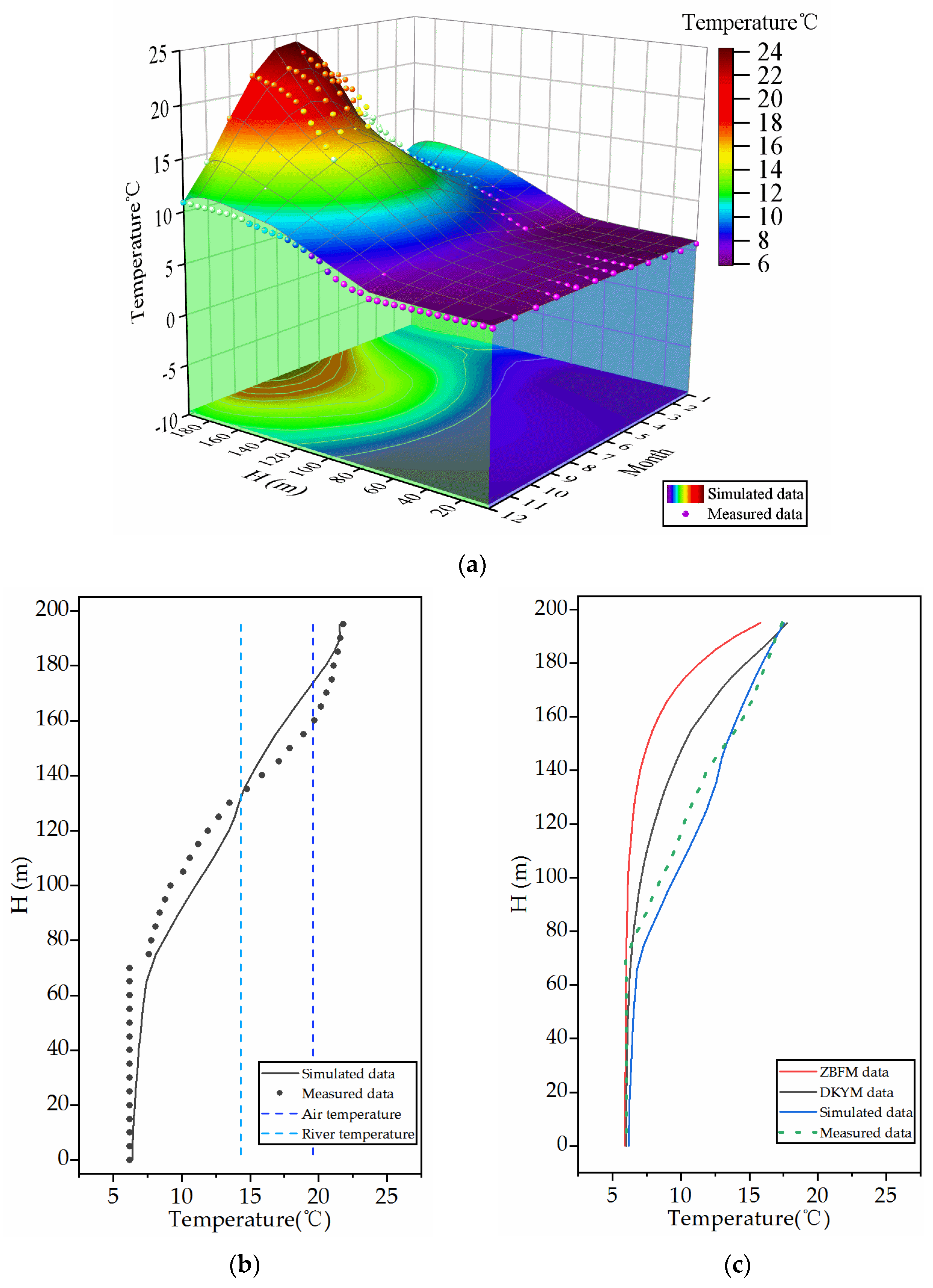
3.2. Analysis of Model Results

Using the parameters above to simulate the temperature of the water in Xulong, the results are shown in Figure 4 and Figure 5:

Figure 4 shows the temperature duration curves of several typical water depths. It can be seen from the figure that the model fits well for the water temperature of different depths. It can also be seen that the water temperature at the surface is relatively high, and the peak temperature appears at a time similar to that of the river water temperature. With the increase in depth, the variation of water temperature decreases with a time lag phenomenon, and the lag phenomenon becomes more obvious as the depth increases. This is because the heat transfer and diffusion along the depth direction, gradually become weaker. At the bottom of the reservoir, the temperature varies slightly, and remains around 6 °C all year round.

Figure 5a clearly demonstrates the changes in the temperature of the water due the variation in depth based on our model. Due to the limited space, Figure 5b only lists the comparison between the simulated and measured data in the month of September. Figure 5c shows the results of three different methods for water temperature. It can be seen from the figure that the method we proposed fits the water temperature better. The two empirical methods are close to an exponential function and cannot accurately describe the variation of the water temperature in the reservoir with depth. After data analysis, the maximum absolute error occurs at 75 m underwater, which is 2.9 °C. The mean error, mean square error, and root mean square error are 0.8 °C, 0.9 °C, and 1.0 °C, respectively. The NSE of I1DM is 0.92, very close to 1. NSE is a parameter that characterizes the quality of the model, and NSE ranges from negative infinity to 1. The closer NSE is to 1, the better the quality of the model and the higher the reliability of the model. When NSE is close to 0, it indicates that the results from the model are close to the average level of the observed values. If NSE is much less than 0, the model is not credible. In conclusion, combined with the error data in Figure 5 and

Table 3. Analysis of error for the whole year (°C).

Parameter	Mean Difference				Root Mean Square				NSE				Time
Method	Xulong	Xiluodu	Jiexu	Sanhekou	Xulong	Xiluodu	Jiexu	Sanhekou	Xulong	Xiluodu	Jiexu	Sanhekou	-
DKYM	1.7	1.1	2.0	3.0	2.5	1.7	2.6	3.6	0.89	0.81	0.64	0.20	<1 min
ZBFM	2.5	1.5	1.1	2.3	3.4	2.3	1.3	2.9	0.78	0.61	0.84	0.50	<1 min
I1DM	0.8	0.8	1.0	1.0	1.0	1.4	1.0	1.5	0.92	0.86	0.91	0.88	<1 min
MIKE3	0.7	0.8	0.9	0.9	0.9	1.1	0.9	1.3	0.93	0.93	0.94	0.90	>3 h

, I1DM has a better simulation effect on the water temperature in the reservoirs, and can reveal the distribution characteristics and variation trends of the water temperature.

$$\mathrm{NSE}=1-\frac{\sum {\left(T_{measured}-T_{simulated}\right)}^2}{\sum {\left(T_{measured}-\overline{T_{simulated}}\right)}^2}$$

3.3. Simulation of the Bottom Slag

The change of the water temperature of the reservoir directly affects the displacement, stress, and water quality of the dam project. The water storage process of the reservoir will affect the water temperature at the bottom. If the water storage time is in the cold season, because the earth and river water temperature are low, the low temperature water will directly accumulate at the bottom of the reservoir at the front of the dam, which will cause the temperature at the bottom to be too low in the early stage. At especially high altitudes or high latitudes, this phenomenon is more pronounced.

On the one hand, the low temperature water increases the temperature difference between the inside and outside of the concrete on the upstream dam surface, and on the other hand, it cools the dam concrete too quickly. These two situations can easily lead to the appearance and expansion of temperature cracks in the dam. Some concrete gravity dams and arch dams located in areas which are extremely cold use the method of bottom slag at the front of the dam in the temperature control and crack prevention design avoid the cold shock of the low temperature water on the concrete of the upstream dam surface [39]. The theory is to prevent the occurrence of temperature cracks at the dam heel by increasing the stable temperature of the strong restraint part of the dam foundation [40,41]. In this paper, the model is used to simulate the bottom slag based on the varying thicknesses in the Xulong project, and the results are shown in Figure 6.

The temperature comparison of bottom slag with a thickness of 40 m (∆2095–∆2135) and no bottom slag is shown in Figure 6. It can be seen that the bottom slag can increase the temperature of the bottom of the reservoir within a certain range. The simulated results agree with the measured data, with an average difference of 0.51 °C. Figure 7 illustrates the water temperature distribution characteristics of bottom slag with various thicknesses. We also simulated bottom slag with a thickness of 50 m (∆2095–∆2145) and 60 m (∆2095–∆2155). It can be seen from the figure that the greater the thickness of the slag, the greater the increase in the temperature at the bottom of the reservoir. When the thickness is 40 m, 50 m, and 60 m, the temperature increases by 5.2 °C, 5.5 °C, and 6.0 °C, respectively. As the thickness of the slag increases, the affected range also increases, roughly 20 m upward from the top of the slag. As the bottom of the slag is affected by the temperature of the earth, so the temperature drops. To sum up, bottom slag is an effective way to increase the boundary temperature at the concrete dam heel, and the temperature can be increased by 5–6 °C.

4. Analysis of Different Water Temperature Models

The simulation methods of water temperature in the reservoir can be roughly divided into two categories—the empirical equation method and numerical algorithms. In this section, DKYM and ZBFM of the empirical equation method and the 3D numerical algorithm in the MIKE3 software are selected to compare with the model I1DM. We compared the simulation results of each model with the measured water temperature data and analyzed the accuracy and applicability of each method, describing the characteristics of each method.

4.1. Characteristics of Each Water Temperature Method

The empirical equation method was summarized by researchers on the basis of analyzing and studying a large amount of measured data. It is not only easy to apply, but the parameters required are also easy to obtain. As long as the temperature of the water at the bottom and at the surface of the reservoir are known, the empirical method can calculate the water temperature distribution each month. It is mainly used for preliminary prediction of the water temperature of the reservoir when the information of the reservoir is limited. As the parameters are empirical, they need to be determined according to the similar projects that have been built. When there is a lack of engineering projects with high similarity, it will be difficult to determine the parameters, and the accuracy is low, which will naturally affect the accuracy of the water temperature simulation.

Numerical algorithms are divided into 1D, 2D, and 3D numerical models, which can assess the influence of many factors on the water temperature of the reservoir (such as topographic conditions, climate, reservoir regulation, water discharge, human factors, etc.). Numerical algorithms are rigorous in theory, focusing on the simulation of the water temperature of a reservoir when operating, mainly for ecosystem and water quality monitoring. Taking the 3D mathematical model of the MIKE3 software as an example, the model needs to collect a large amount of data during the operating stage of the reservoir and perform a lot of parameter calibration work. The boundary conditions and parameters that need to be provided include more than 20 parameters such as topographic data, heat exchange boundary, turbulent viscosity coefficient, riverbed roughness, and the Smagorinsky parameter. This shows that the application of numerical algorithms is complex and requires a lot of preliminary work.

4.2. Comparison of Simulation Results

Table 3 shows that different models have different simulation accuracy for different reservoirs. Overall, the empirical methods (DKYM and ZBFM) is the least accurate, and the accuracy of the I1DM in this paper is similar to the MIKE3 model. Based on the results obtained through the algorithm described in this paper, the average differences for the temperature of the water are 0.8 °C, 0.8 °C, and 1.0 °C and the root mean squares are 1.0 °C, 1.4 °C, and 1.0 °C. Both are lower than the empirical algorithm, which means that the error of method in this paper is smaller and the distribution is more uniform compared with the empirical method. The NSE of different reservoirs are 0.92, 0.86, and 0.91, which are closer to 1 than that of the empirical method, indicating that the simulation of the water temperature of the reservoir by the method we proposed is more realistic.

Compared with the 3D algorithm, the accuracy of this method is slightly worse. However, under the same configuration conditions (Intel i7-6700, 3.40 GHz, SSD980), the efficiency of the method in this paper is much higher than that of the 3D algorithm. The calculation time of the method in this paper is less than one minute for the four reservoirs. Due to the consideration of numerous parameters and the complexity of calculation, the time of the 3D model would more than 3 h, and this time increases as the grid grows.

Figure 8 shows the comparison of the simulation accuracy of each vertical one-dimensional algorithm, coefficient of accuracy $\mathsf{\mu }=1-\frac{\sum \left|T_{measured}-T_{simulated}\right|}{\sum T_{measured}}$. It can be seen from Figure 8 that the accuracy coefficient of I1DM for water temperature in each month is greater than that of the two empirical algorithms. Combining the water level data in

Table 4. Reservoir operating water level (altitude, m).

Reservoir Name	Jan	Feb	Mar	Apr	May	Jun	Jul	Aug	Sept	Oct	Nov	Dec
Xulong	2302	2302	2302	2302	2302	2302	2302	2302	2302	2302	2302	2302
Xiluodu	595	590	575	560	540	555	560	560	590	600	600	600
Jiexu	3374	3374	3370	3369	3367	3369	3369	3369	3369	3369	3370	3372
Sanhekou	634	634	634	634	634	634	634	634	634	634	634	634

and the accuracy coefficient chart of each month, the simulation accuracy of each algorithm in 12 months is relatively uniform for both the Xulong project and Sanhekou project, with stable water levels and little change in inflow throughout the year. As the inflow rates of Xiluodu project and Jiexu project have a big variation within the year, in order to meet the requirements of flood control, it is necessary to release water in advance before the flood season (June–September). The water levels of the Xiluodu and Jiexu reservoirs vary greatly within a year. On the one hand, the change of water level will enhance the mixing effect of reservoir water; on the other hand, a large amount of river water during the flood season will cause the temperature of the reservoir to change in a short period of time. In this case, the empirical formula has a low simulation accuracy as it cannot take the inflow, outflow, and the fluctuations in water levels into account. The highest$\mathsf{\mu }$that the Xiluodu project and Jiexu project simulated was 0.92 and 0.90, respectively, and the lowest$\mathsf{\mu }$was 0.26 and 0.36, respectively, so the simulation accuracy of the empirical method fluctuates greatly each month.

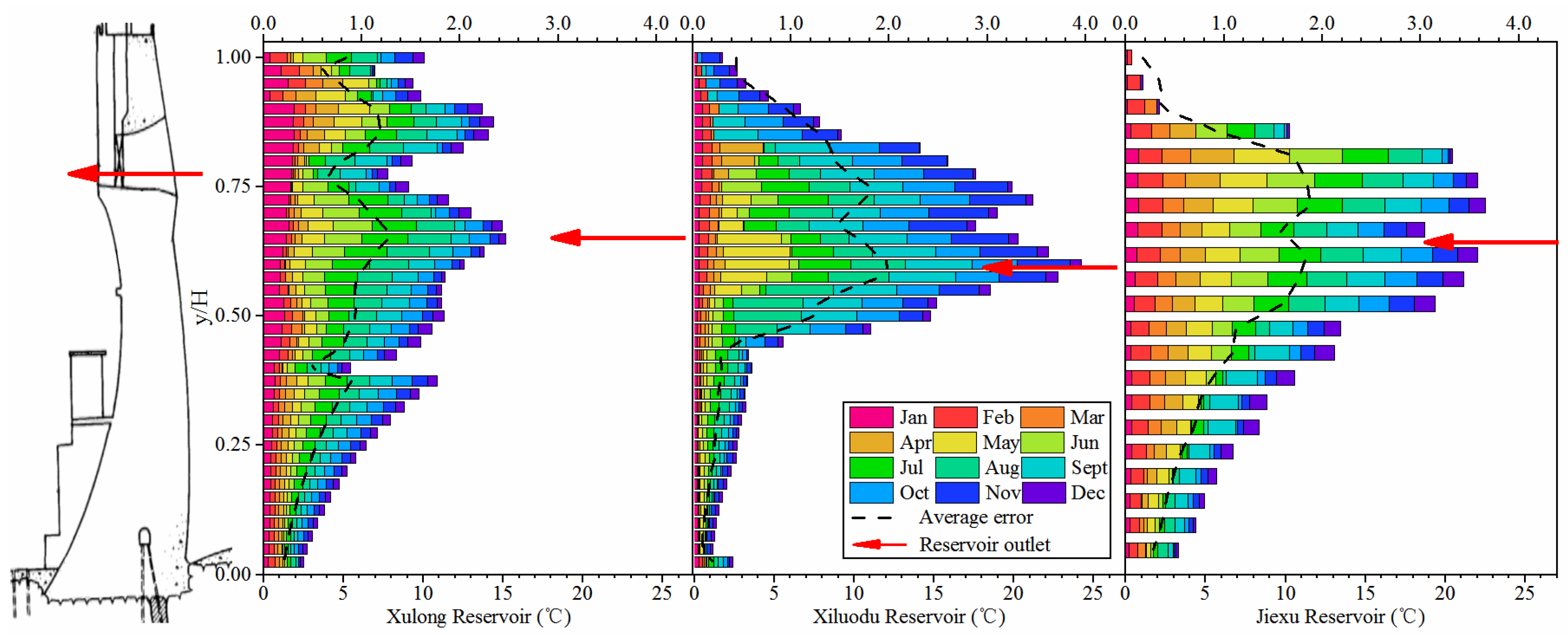
4.3. Analysis of the Error in Vertical Direction of I1DM

As the water level of the Xiluodu project and the Jiexu project decreased before the flood season, there were no error data at certain depths. It can be seen from Figure 9 that the results of the Xulong Reservoir with a constant water level throughout the year are significantly better than those of the Xiluodu Reservoir and the Jiexu Reservoir with changing water levels. This is consistent with the results of the analysis in Figure 8. From the error analysis of the three reservoirs in each month, it can be seen that from May to October, due to the increase in water inflow during the flood season, the prediction error also increases. The maximum total error of each depth of Xulong Reservoir is 15.1 °C at the altitude of 2225 m, the maximum total error of each depth of Xiluodu Reservoir is 24.3 °C at the altitude of 495 m, and the maximum total error of each depth of Jiexu Reservoir is 22.8 °C at the altitude of 3339 m. All the above-mentioned altitude positions are near the reservoir outlet. It can be concluded that the errors are mainly concentrated near the outlet, and the errors between the surface and the bottom are small. The errors show a trend of increasing towards the outlet of the reservoir. The discharge of the reservoir will affect the water status near the outlet. Due to the frequent dispatch of the reservoir, the water flow near the outlet is complicated. So, the error of the water temperature is mainly concentrated around this range.

5. Conclusions

We improved the vertical one-dimensional numerical algorithm of reservoir water temperature and completed the compilation of the corresponding program. The improved algorithm can not only take factors such as reservoir operation mode, reservoir water level change, inflow water temperature, reservoir geometry, and solar radiation, etc. into account, but it can also predict distribution of the water temperature under the condition of bottom slag at the front of the dam.

• The NSE of the water temperature simulation results of the three different reservoirs are all above 0.85, and the average difference is below 1.0 °C, which has a high reliability. It can be concluded that the algorithm is suitable for predicting the water temperature at the front of the dam for reservoirs in various scales and modes of operation.
• Compared with the empirical method, this algorithm is more thorough in theory, considers more working conditions, and has more accurate simulation results. Compared with the three-dimensional numerical algorithm, this algorithm is more efficient and easier to use.
• The model proposed in this paper can be seamlessly embedded in the simulation program for concrete dam temperature control. More accurate temperature boundary conditions are provided for the simulation program without affecting the overall efficiency. The reliability of the simulation results of stress state in the crack-prone areas of the upstream surface is further improved, and it has important engineering significance for the temperature control and crack prevention design of large concrete dams.

References

1. Aniskin, N.; Nguyen, T.C. Influence factors on the temperature field in a mass concrete. E3S Web Conf. 2019, 97, 05021. [Google Scholar] [CrossRef]
2. Briffaut, M.; Benboudjema, F.; Torrenti, J.M. Numerical analysis of the thermal active restrained shrinkage ring test to study the early age behavior of massive concrete structures. Eng. Struct. 2011, 33, 1390–1401. [Google Scholar] [CrossRef]
3. Silva, C.M.; Castro, L.M. Hybrid-mixed stress model for the nonlinear analysis of concrete structures. Comput. Struct. 2005, 83, 2381–2394. [Google Scholar] [CrossRef]
4. Wang, H.B.; Qiang, S.; Sun, X. Dynamic Simulation Analysis of Temperature Field and Thermal Stress of Concrete Gravity Dam during Construction Period. Appl. Mech. Mater. 2011, 90–93, 2677–2681. [Google Scholar] [CrossRef]
5. Zhang, G.; Liu, Y.; Yang, P. Analysis on the causes of crack formation and the methods of temperature control and crack prevention during construction of super-high arch dams. J. Hydroelectr. Eng. 2010, 29, 45–51. [Google Scholar] [CrossRef]
6. Morrison, J.; Quick, M.C.; Foreman, M. Climate change in the Fraser River watershed: Flow and temperature projections. J. Hydrol. 2002, 263, 230–244. [Google Scholar] [CrossRef]
7. Nsiri, I.; Tarhouni, J.; Irie, M. Modeling of Thermal Stratification and the Effect on Water Quality in Four Reservoirs in Tunisia. Hydrogeol. Hydrol. Eng. 2016, 5, 1. [Google Scholar] [CrossRef]
8. Huber, W.C.; Harleman, D.R.; Ryan, P.J. Temperature prediction in stratified reservoirs. J. Hydraul. Div. 1972, 98, 645–666. [Google Scholar] [CrossRef]
9. Haag, I.; Luce, A. The integrated water balance and water temperature model LARSIM-WT. Hydrol. Processes 2010, 22, 1046–1056. [Google Scholar] [CrossRef]
10. Kong, Y.; Deng, Y.; Tuo, Y. Application of one-dimensional vertical temperature model in Dongjiang Reservoir. Yangtze River 2017, 48, 97–102. [Google Scholar] [CrossRef]
11. Lindenschmidt, K.E.; Carr, M.K.; Sadeghian, A. CE-QUAL-W2 model of dam outflow elevation impact on temperature, dissolved oxygen and nutrients in a reservoir. Sci. Data 2019, 6, 312. [Google Scholar] [CrossRef]
12. Diao, W.; Cheng, Y.G.; Zhang, C.Z. Three-dimensional prediction of reservoir water temperature by the lattice Boltzmann method: Validation. J. Hydrodyn. 2015, 27, 248–256. [Google Scholar] [CrossRef]
13. Yin, T.; Li, Q.; Hu, Y.; Yu, S.; Liang, G. Coupled Thermo-Hydro-Mechanical Analysis of Valley Narrowing Deformation of High Arch Dam: A Case Study of the Xiluodu Project in China. Appl. Sci. 2020, 10, 524. [Google Scholar] [CrossRef] [Green Version]
14. Wang, Q. Prediction of Water Temperature as Affected by a Pre-Constructed Reservoir Project Based on MIKE11. Clean-Soil Air Water 2013, 41, 1–5. [Google Scholar] [CrossRef]
15. Wang, Q.; Zhao, X.; Chen, K. Sensitivity analysis of thermal equilibrium parameters of MIKE 11 model: A case study of Wuxikou Reservoir in Jiangxi Province of China. Chin. Geogr. Sci. 2013, 23, 584–593. [Google Scholar] [CrossRef] [Green Version]
16. He, W.; Lian, J.; Du, H. Source tracking and temperature prediction of discharged water in a deep reservoir based on a 3-D hydro-thermal-tracer model. J. Hydro-Environ. Res. 2018, 20, 9–21. [Google Scholar] [CrossRef]
17. Park, G.G.; Schmidt, P.S. Numerical Modeling of Thermal Stratification in a Reservoir with Large Discharge-to-Volume Ratio1. Jawra J. Am. Water Resour. Assoc. 2010, 9, 932–941. [Google Scholar] [CrossRef]
18. Wormleaton, P.R.; Hadjipanos, P. Flow Distribution in Compound Channels. J. Hydraul. Eng. 1985, 111, 357–361. [Google Scholar] [CrossRef]
19. Lin, G.F.; Wu, M.C. An RBF network with a two-step learning algorithm for developing a reservoir inflow forecasting model. J. Hydrol. 2011, 405, 439–450. [Google Scholar] [CrossRef]
20. Lin, G.F.; Wu, M.C.; Chen, G.R. An RBF-based model with an information processor for forecasting hourly reservoir inflow during typhoons. Hydrol. Processes 2010, 23, 3598–3609. [Google Scholar] [CrossRef]
21. Kim, S. Analysis of the Water Circulation Structure in the Paldang Reservoir, South Korea. Appl. Sci. 2020, 10, 6822. [Google Scholar]
22. Li, X.; Qiu, J.; Shang, Q. Simulation of Reservoir Sediment Flushing of the Three Gorges Reservoir Using an Artificial Neural Network. Appl. Sci. 2016, 6, 148. [Google Scholar] [CrossRef] [Green Version]
23. Tomasz, G.D. Computational Fluid Mechanics and Heat Transfer. AIAA J. 2013, 51, 2751. [Google Scholar] [CrossRef]
24. Ogedengbe, E. Non-inverted skew upwind scheme for numerical heat transfer and fluid flow simulations. Diss. Abstr. Int. 2006, 68, 0586. [Google Scholar]
25. Zakonnova, A.V.; Litvinov, A.S. Analysis of Relation of Water Temperature in the Rubinsk Reservoir with Income of Solar Radiation. Hydrobiol. J. 2017, 53, 77–86. [Google Scholar] [CrossRef]
26. Chang, J.Q. Research on Vertical Distribution of Water Temperature in Different Regulation Reservoirs. Adv. Mater. Res. 2014, 3248, 3190–3197. [Google Scholar] [CrossRef]
27. Lee, H.; Chung, S.; Ryu, I. Three-dimensional modeling of thermal stratification of a deep and dendritic reservoir using ELCOM model. J. Hydro-Environ. Res. 2013, 7, 124–133. [Google Scholar] [CrossRef]
28. Chen, Y.C.; Kao, S.P. Velocity distribution in open-channel flows with submerged aquatic plant. Hydrol. Processes 2011, 25, 2009–2017. [Google Scholar] [CrossRef]
29. Shu, A.P.; Liu, Q.Q.; Fei, X.J. Unified laws of velocity distribution for sediment laden flow with high and low concentration. J. Hydraul. Eng. 2006, 37, 1175–1180. [Google Scholar] [CrossRef]
30. Lu, J.; Zhou, Y.; Zhu, Y. Improved formulae of velocity distributions along the vertical and transverse directions in natural rivers with the sidewall effect. Environ. Fluid Mech. 2018, 18, 1491–1508. [Google Scholar] [CrossRef]
31. Song, B.; Schmalz, N.F. Improved structure of vertical flow velocity distribution in natural rivers based on mean vertical profile velocity and relative water depth. Nord. Hydrol. 2018, 49, 878–892. [Google Scholar] [CrossRef]
32. Li, X.; Yan, H.B.; Xu, Y. Discussion on New Formula of Velocity Distribution in Rectangular Open Channel. Yangtze River 2021, 39, 3. [Google Scholar]
33. Ahmed, A.; Said, M.; Mohamed, T. Stability Criterion for Uniform Flow in Open Channel Cross Sections with Different Shapes. J. Irrig. Drain. Eng. 2020, 146, 40. [Google Scholar] [CrossRef]
34. Simpson, J.J.; Paulson, C.A. Mid-ocean observations of atmospheric radiation. Q. J. R. Meteorol. Soc. 2010, 105, 487–502. [Google Scholar] [CrossRef]
35. Gueymard, C.A. The sun’s total and spectral irradiance for solar energy applications and solar radiation models. Sol. Energy 2004, 76, 423–453. [Google Scholar] [CrossRef]
36. Wilfried, B. On a derivable Equation for long-wave radiation from clear skies. Water Resour. Res. 2010, 32, 742–744. [Google Scholar] [CrossRef]
37. Swinbank, W.C. Long-wave radiation from clear skies. Q. J. R. Meteorol. Soc. 2010, 89, 339–348. [Google Scholar] [CrossRef]
38. Chang, X.; Liu, X.; Wei, B. Temperature simulation of RCC gravity dam during construction considering solar radiation. Eng. J. Wuhan Univ. 2006, 39, 26–29. [Google Scholar] [CrossRef]
39. Zhu, Z.Y.; Qiang, S.; Liu, M.Z. Cracking Mechanism of Long Concrete Bedding Cushion and Prevention Method. Adv. Mater. Res. 2011, 163–167, 880–887. [Google Scholar] [CrossRef]
40. Zhu, Z.Y.; Qiang, S.; Liu, M.Z. Cracking Mechanism of RCC Dam Surface and Prevention Method. Adv. Mater. Res. 2011, 295–297, 2092–2096. [Google Scholar] [CrossRef]
41. Yuan, M.; Qiang, S.; Xu, Y. Research on Cracking Mechanism of Early-Age Restrained Concrete under High-Temperature and Low-Humidity Environment. Materials 2021, 14, 4084. [Google Scholar] [CrossRef]
Figure 1. Schematic diagram of the simulation model.
Applsci 12 05870 g001
Figure 2. The temporal and spatial distribution of the measured water temperature of Xulong.
Applsci 12 05870 g002
Figure 3. Duration curves of meteorological and hydrological data.
Applsci 12 05870 g003
Figure 4. Temperature at different depths of Xulong. (a) Water depth 20 m. (b) Water depth 40 m. (c) Water depth 100 m. (d) Bottom of reservoir.
Applsci 12 05870 g004
Figure 5. Comparison between simulation data and measured data. (a) Comparison between simulation data and measured data. (b) September. (c) Average temperature.
Applsci 12 05870 g005
Figure 6. Water temperature of Xulong Reservoir (bottom slag 40 m).
Applsci 12 05870 g006
Figure 7. Water temperature of bottom slag of different thicknesses in Xulong Reservoir.
Applsci 12 05870 g007
Figure 8. Comparison of precision coefficients for each month. (a) Xulong. (b) Xiluodu. (c) Jiexu. (d) Sanhekou.
Applsci 12 05870 g008
Figure 9. The total error of each depth in the vertical direction of the three reservoirs.
Applsci 12 05870 g009