Scanning Inductive Thermographic Surface Defect Inspection of Long Flat or Curved Work-Pieces Using Rectification Targets

Featured Application

In this work, checkerboard grids, made from different materials, are used to improve inductive scanning pulse phase thermography (SPPT) for detecting surface defects and to create panoramic images for long specimens with a non-flat surface.

Abstract

Inductive thermography is an NDT method, which can be excellently used to inspect long metallic specimens (such as railway tracks) to detect surface defects. Aiming at the inspection of railway tracks in service with a movable setup, the method had to be advanced from a stationary application to a scanning setup. This work presents methods for using calibration targets for rectification, in order to improve the quality of the resulting images. Two scanning techniques are presented for detecting different types of rolling contact fatigue (RCF) defects on rail pieces. In the case of the first method, separate stationary inductive pulsed measurements are carried out for the segments of a long sample and the results are stitched together to one panoramic image of the whole specimen (“stop-and-go”). Since the surface of the rail piece is curved, rectification of the surface with a flexible grid is necessary to generate seamless panoramic images. In the case of the second method, a specimen is moved with constant speed underneath the induction coil. For the detection of shallow surface cracks, the infrared camera has to have a view of the surface during the heating; therefore, the camera is placed behind the coil but tilted towards a position below the induction coil. In order to be able to evaluate phase images from the temporal temperature change, a checkerboard grid as a rectification target is used. It is also analyzed how the chosen IR camera frame rate and the motion speed affect the scanning result.

1. Introduction

In the case of inductive thermography, a short inductive heating pulse in the range of 0.05–1 s is applied to the work-piece and the surface temperature is recorded during and after the heating pulse by an infrared (IR) camera. Surface defects deflect the induced eddy currents and disturb the heat diffusion; therefore, the defects in metallic materials can be excellently detected by analyzing the infrared images [1,2,3,4,5,6]. In addition, this method has the advantage compared to other methods such as magnetic particle testing or penetration testing that it also provides information about the defect depth and about the inclination angle of a surface crack [1].

Metallic surfaces often have a low emissivity value and inhomogeneous surface properties. Evaluating only one infrared image, e.g., at the end of the heating pulse, is strongly affected by this inhomogeneity and also by the inhomogeneity of the heating. This could cause false detections or on the other hand, missing detection of defects. However, recording a whole infrared sequence and evaluating the temporal change in the temperature provides the advantage of suppressing the inhomogeneity effects and it reduces the background noise in the images, resulting in a higher detection reliability. For the evaluation of the infrared sequence, often Fourier transformation is used to calculate a phase image, which is then used to localize and to characterize the defects [7].

For the inspection of long work-pieces, scanning in a stop-and-go way, which is also called step scanning [8], can be used. During one measurement, both the inductor and the recording infrared camera are stationary and after one measurement, either the work-piece or the heat source together with the IR camera are moved further to the next position. Afterwards, the separate measurement results are stitched together to one panorama image [8,9]. In this paper, a method is presented to optimize this technique by applying a calibration object for rectifying the images. As we have applied this method to a rail piece where the defects occur at the curved surface of the gauge line, the calibration object was also used to reduce errors in the stitching caused by the rail curvature.

Another possibility for the inspection of long pieces is a scan with continuous motion [9,10,11,12], where either the work-piece is moved with a constant speed and the heat source together with the infrared camera are stationary, or the reverse. During this relative motion, the infrared camera always records the temperature of different parts of the inspected work-piece; therefore, an additional step is necessary to generate a phase image. The pixels in the recorded infrared images are reorganized in a way, as they belong to the same position of the work-piece, as it would be the case for a stationary measurement. This allows for the application of the same evaluation method of Fourier transformation, as it has been developed for stationary measurements [11].

The scanning pulse phase thermography, SPPT [11], works very well for the detection of subsurface defects. In this case, only the temperature changes after the heating pulses are evaluated. The heat is generated due to the induced eddy currents in a thin depth at and below the surface and the heat travels into the body. If there is a defect, then the heat diffusion is disturbed and the perturbation in the surface temperature can be observed with a time delay after the heating pulse. Therefore, the most relevant information regarding the defect detection is contained in the temperature change recorded after the heating pulse [13]. For surface cracks, the situation is different and the most important part of the information is included in the temperature change during the heating, as the perturbation due the surface crack occurs instantly at the surface. If the induction coil during the scanning covers the surface, then due to this occlusion, the infrared camera cannot record the temperature during the heating. A method has been developed, which is presented in this paper, where the camera is mounted tilted at an angle to the specimen’s surface, so that the specimen’s movement underneath the induction coil is in frame. This allows for the recording of the temperature during the heating process. Furthermore, a calibration object is used to rectify the infrared camera images, in order to allow for the reordering of the pixels and the calculation of the phase image.

The structure of this paper is the following: after this introduction, the rail pieces are described, which we used to demonstrate the new developments for the inductive scanning thermography technique. Then, the two experimental setups for stop-and-go and for continuous scanning are described in Section 3. The used calibration objects and the applied rectification procedures are presented in Section 4. The performed measurements of the two rail pieces in stop-and-go motion and in continuous motion are described in the fifth and sixth Section. The results of the presented method are then discussed and summarized in Section 7.

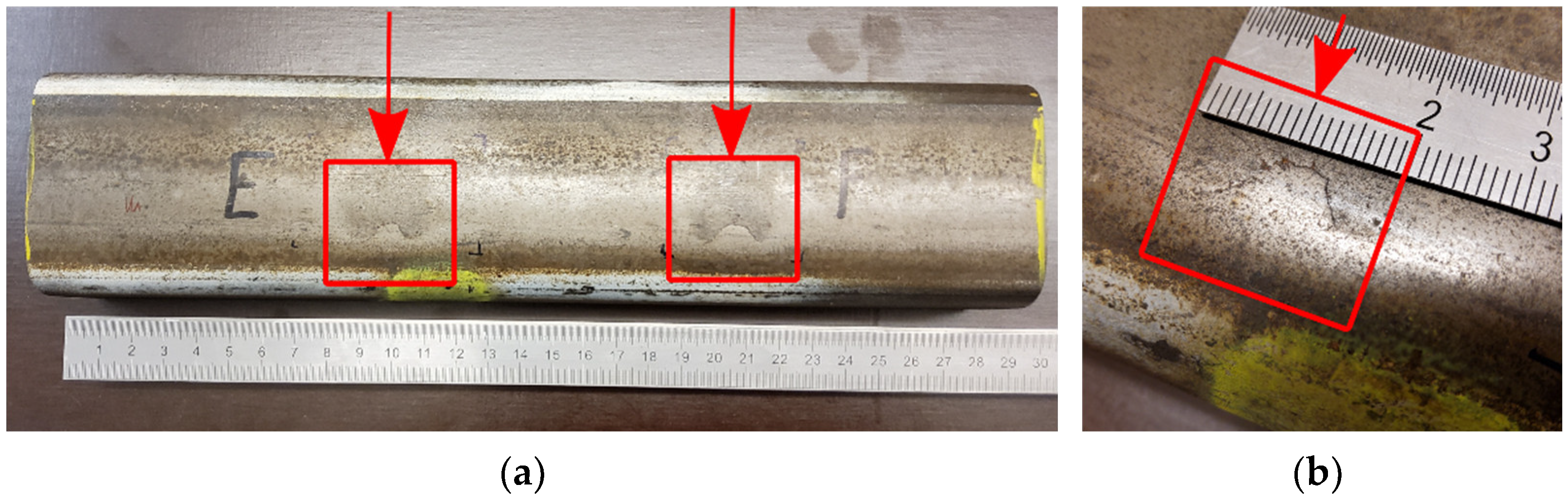
2. Description of Specimens

To demonstrate the advantages of the scanning inductive thermography, two rail pieces with rolling contact fatigue (RCF) defects were used. As described in a recent publication, head checks and squats are common defects on rails, stemming from rolling contact fatigue (RCF) [9].

Head checks are a material fatigue phenomenon caused by the high contact stresses between the wheel and the gauge corner of the rail that occur in sections of track with a curve radius between 500 m and 3000 m. They appear as fine surface cracks that occur at discrete intervals that grow into the rail head with a very shallow entry angle (10–30 degrees). Squats are rolling contact fatigue (RCF) defects that occur in straight or (gently) curved track within the running band on the rail head, where the rail is heavily sheared. This specific defect phenomenon is thought to be initiated via small parts of hard material (such as pieces of track ballast) that are caught between the rail and wheel and cause certain cracks to grow. The crack then preferentially grows in the direction of the heavily sheared surface layer; this generates the characteristic round shape of the squat. For a more detailed description of head checks and squats, one can refer to [9] and the references therein.

A 250 mm long piece of rail with head checks on the gauge corner (RP01; see Figure 1) was used for the scanning in stop-and-go technique. The rail piece was provided from voestalpine Rail Technology GmbH and it is a cut out piece of a decommissioned pearlitic rail from the Austrian railway system. A characterization of the head checks on this specific rail piece was published in [9]. The average distance between the head checks was determined as 2.54 mm and an average length of head checks as 17.1 mm.

The specimen used for continuous scanning is a 300 mm long pearlitic rail piece with squats (RP02; see Figure 2). The specimen has two large squats, which are clearly visible and some small and shallow cracks in the earlier stages of crack progression. These ones are not or only barely visible. The specimen is also a cut-out part of a decommissioned rail piece found in the Austrian railway system, provided by voestalpine Rail Technology GmbH.

Table 1. Description of the two rail pieces.

Short Name	Damage Type	Length of Rail Piece	Used for
RP01	Head checks	250 mm	Stop-and-go scanning
RP02	Squats	300 mm	Continuous scanning

presents a short summary of both rail pieces and shows the short names that will further be used in this work to reference the specimens.

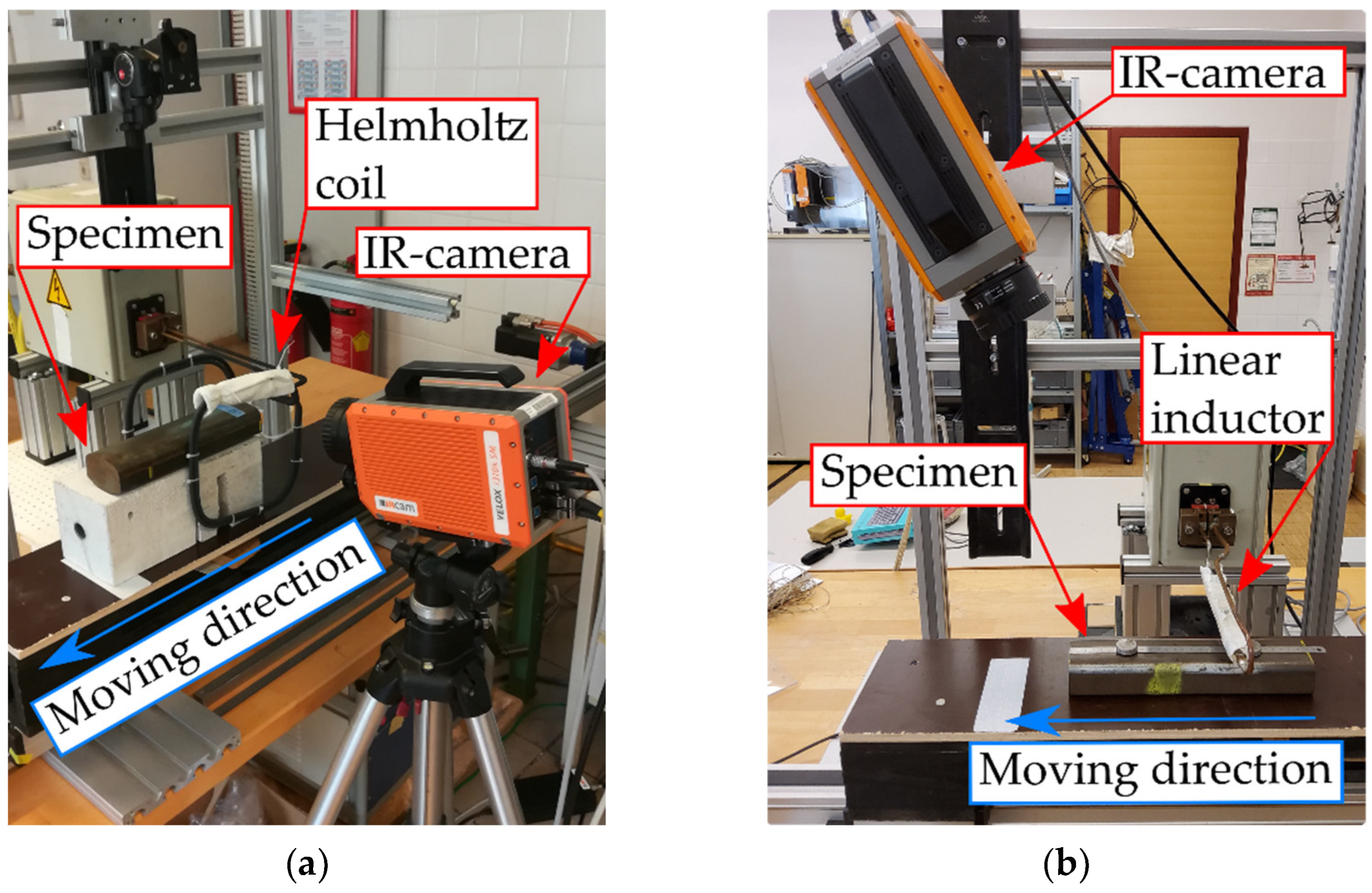
3. Experimental Setup

In the experimental setups, a high frequency (HF) induction generator with 5 kW power was used. Depending on the attached inductor, the excitation frequency is in the range between 100 and 200 kHz. The specimen is placed on a linear table and moved via a linear actuator providing motion speeds up to 250 mm/s.

For the measurements, the IRCAM Velox 1310k SM, a cooled infrared camera with an InSb detector, was used. In standard full-window mode, the camera records 180 images per second with 1280 × 1024 pixels. By changing to binning mode, the number of pixels is reduced to 640 × 512 for the same field-of-view (FOV), as 2 × 2 pixels are recorded together. In binning mode, the frame rate is increased to 600 images per second. To test the limits of the new SPPT approach, additional measurements were carried out with a much slower µ-bolometer camera (FLIR A615), recording 50 images per second with 640 × 480 pixels. This camera has the option of increasing its frame rate to 100 or 200 images per second by restricting the number of recorded pixel rows to 240 or 120, respectively. A µ-bolometer camera is slower and has lower temperature resolution than the cooled InSb detector, but it does not require cooling, which makes this camera type more advantageous in an industrial environment.

3.1. Setup for Stop-and-Go Technique

Figure 3a shows the setup for scanning in the stop-and-go approach. A so-called Helmholtz coil is used to heat the specimen RP01. This type of coil induces the eddy current almost homogenously in a larger region inside the coil. Therefore, it is often used in stationary pulse phase thermography.

The camera is placed on one side of the linear table looking at the gauge corner of the rail piece inside the Helmholtz coil. The distance between camera and specimen is approximately 250 mm. The specimen is positioned so that a motion through the coil is possible and eddy current excitation inside the coil heats the surface of the rail gauge corner between 0.8 and 1.5 K during a pulse length of 0.3 s.

3.2. Setup for Continuous Scanning

The setup for continuous scanning is shown in Figure 3b. RP02 is positioned on the linear table and the line heating source is placed above the rail piece and perpendicular to the motion direction. The line heating source is equipped with an additional field concentrator, which focuses the magnetic field into the specimen below. The overall width of the inductor is 20 mm.

The camera is positioned behind the induction coil tilted in a 60-degree angle to the surface of the specimen. The distance between the induction coil and the specimen beneath was set to approximately 40 mm, so that the heated surface area of the specimen below the coil can be viewed and recorded by the IR camera.

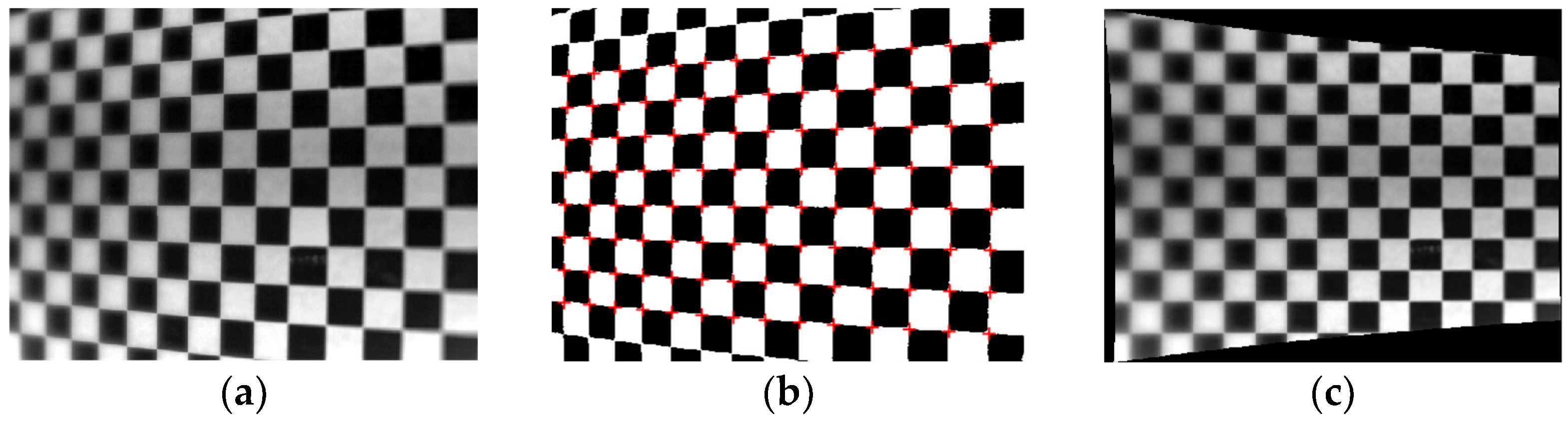
4. Rectification with Checkerboard Pattern

For the measurements presented in this work, two different types of checkerboard grids are used. In both cases, a single calibration image with the grid is taken before the measurements. This calibration image is then used to create a transformation, which is applied to the subsequent measurements. This transformation warps the checkerboard grid so that all the chessboard squares are the same size. The goal is to transform images and sequences in such a way that the field of view becomes rectified without any distortion due to the perspectivity or due to the curvature of the surface.

4.1. Foldable Checkerboard for Stop-and-Go Scanning

The rail gauge line of RP01 has a curved surface. Since the goal is to recognize the curvature of the specimen in the infrared image, a bendable calibration target is necessary. The checkerboard grid was printed on a piece of paper using common black printer ink (see Figure 4a). In order to increase the contrast in the IR image between the paper and ink, the grid is warmed with a halogen lamp, as shown in the IR image in Figure 4b.

4.2. Rigid Checkerboard for Continuous Scanning

In the case of continuous scanning, the camera has a strongly perspective view; therefore, a rigid calibration target with good contrast is needed. For SPPT, a metallic plate with a checkerboard grid made of adhesive film is used. The adhesive film was stuck on the metal plate and the checkerboard grid was cut out afterwards (see Figure 4c). As the adhesive film has a higher emissivity value than the shiny metal surface, this checkerboard grid has a high contrast in the infrared image. On the other hand, it is not bendable. In order to increase the contrast between metal plate and adhesive film, the metallic plate was heated with a heat gun before the calibration image was taken (as shown in the IR image in Figure 4d).

4.3. Computation of the Transformation Matrix

The next step is to determine the rectification transformation from the IR images of the calibration object. Figure 5a shows a calibration infrared image as it is recorded by the IR camera. To create a transformation, first the software marks the corners of the checkerboard grid in the image. Using MATLAB’s image processing toolbox, a binary image of the recorded calibration image is computed. By further processing, wrong spots in the binary image are eliminated using morphological operators. MATLAB provides a function to detect checkerboard points in an image, which is often used for camera calibration. This function detects n × m checkerboard points in the binary image (see Figure 5b).

In order to be able to calculate the rectification, a further set of points with n × m size and with quadratic shape must be generated. The rectification algorithm will transform the localized distorted n × m points to this regular and quadratic pattern. The lowest point on the right side of the original grid is used as a starting point. The mean distance is computed by comparing distances of the lowest row in the original grid. With the starting point and with the mean distance, the new checkerboard points are generated. A geometrical fit of the original and the generated point matrix is computed, using a third order polynomial fitting. The resulting transformation consists of the polynomial coefficients A and B, which are used to determine U and V in the inverse transformation, where U and V are the x- and y- coordinates of the points in the original coordinate system [14]. The transformation can now be applied on images of the same size as the calibration image and each pixel is shifted according to the polynomial transformation. Figure 5c shows the rectification of the original grid, after the transformation is applied to the calibration image. This transformation is saved and used on further images of the recorded sequences. The used mean distance is also saved, since it provides the information about the resolution of the transformed image in pixel/mm.

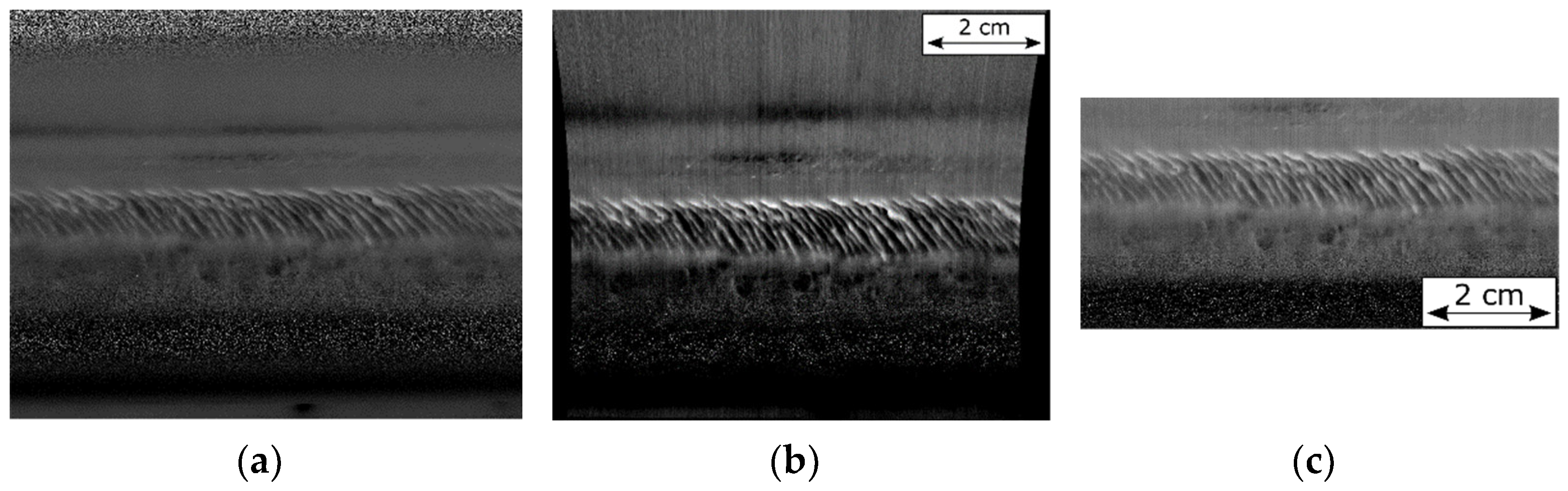
5. Results for Scanning in a Stop-and-Go Method

5.1. Recording Separate Measurements

Scanning in a stop-and-go motion was performed on RP01. Since head checks occur in narrow distances to each other, a high pixel-resolution is necessary to evaluate this type of defect. Therefore, stationary measurements are preferable, which led to this type of scanning technique.

For scanning with the stop-and-go technique, five measurements were carried out on RP01. The recorded IR sequences include the heating and the cool down of the specimen surface during and after the 0.3 s inductive heating pulse. The size of the recorded images is 1280 × 1024 pixels and approximately 80 mm of the rails gauge corner is in the FOV in one stationary measurement. The linear table was then shifted 60 mm between each stationary measurement, resulting in an overlapping area of approximately 20 mm for consecutive measurements. Each separate measurement was evaluated using a pixelwise Fourier transformation, resulting in five phase images (see Figure 6a).

5.2. Rectification Transformation

The next step is to transform the phase images using the transformation, computed previously based on the calibration object. Figure 6b shows that the upper and lower parts of the rectified image are stretched out, whereas in the middle of the image, the sides are pushed inward due to the rectified curvature. Therefore, the phase image is cropped on all sides to the relevant range, resulting in a 1249 × 607 pixel image (see Figure 6c). As the curvature of the rail gauge is rectified in this image, it can be used to calculate the panoramic view.

5.3. Stitching to One Panoramic Image of the Single Images

In order to correctly position the separate transformed phase images on a common canvas, the information about the shifting between the measurements and the resolution, calculated during the computation of the transformation, is necessary. In the presented case, the linear table was moved by 60 mm between the measurements and the calculated resolution was 15.85 px/mm. This means that to align two consecutive phase images, the second image must be shifted by 60 times 15.85 = 951 px to the right side in x-direction. Small misalignments may occur due to the not 100% accurate reproducible shifting during the measurements, which can be recognized in the overlapping areas of two consecutive phase images. To align the images correctly, phase correlation is calculated in those overlapping areas (see Figure 7a). Figure 7b shows that only small shifts in x- and y-direction are computed by the phase correlation algorithm.

Adding together the shift calculated from the motion between the two consecutive measurements and the shift due to the misalignment determined by phase correlation, the images can be placed correctly on a common canvas. In a last step, a linear fading in and out of pixel values in the overlapping regions is added on the phase images (see Figure 8). This fading of the pixel values allows for a smooth transition between the consecutive phase images and a panoramic view can be computed (see in Figure 9).

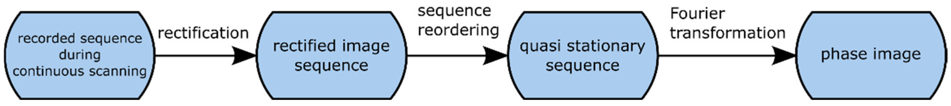
6. Results for Scanning in Continuous Motion

6.1. Continuous Scanning Measurements

This type of scanning is well established and used for detecting subsurface defects by evaluating cooling after a heating source. However, changes in the temperature of surface defects dissipate rather quickly; therefore, it is essential for crack detection to also record during the heating of the specimen. In case of a linear inductor direct recording of the heating is blocked by the heating source, it is necessary to tilt the camera towards the inductor and to rectify the recorded images afterwards.

Several measurements were performed with scanning speeds from 50 mm/s up to 200 mm/s. The camera was set to binning mode with a frame rate of 300 Hz and mounted in a tilted way (see Figure 3b) so that it records the surface temperature of the specimen RP02 while it transits underneath the inductor. In this way, the surface temperature is recorded during the inductive heating and also afterwards during the cool down. On the other hand, due to the tilted camera setup, the image has to be rectified to eliminate the perspectivity.

6.2. Evaluation of Scanning Measurements in Continuous Motion

The evaluation process for measurements in continuous scanning is described in Figure 10. Two transformations of the entire image sequence are necessary to compute a resulting phase image of the whole work-piece.

In the first step, each IR image of the recorded sequence is rectified via transformation, calculated from the calibration image. Figure 11 shows the original recorded IR image in the position as the squat defect is moving through below the inductor. In the camera’s FOV, the inductor is on the left side and the specimen is moved from left to right in x-direction. Due to the first performed transformation, the sides of the images cannot be used and the images are cropped to a size of 623 × 424 pixels. This results in a new image sequence shown in Figure 11b. This sequence looks in a way as if it was recorded by a camera with a perpendicular view of the specimen’s surface, but with the difference that the position below the inductor is visible.

In the next step, this transformed IR sequence is reorganized with the same method as described in an earlier publication [11]. The pixel-columns are shifted and interpolated according to the scanning speed and the camera’s FOV. In this way, a new image sequence is calculated where each pixel corresponds to a real position on the specimen’s surface.

s, the shift of the specimen between two consecutive images of the rectified image sequence, is calculated as follows:

$$s=\frac{v·\overline{x}}{f},$$

(1)

where $v$ is the motion speed in mm/s, $f$ is the camera’s frame rate in Hz and $\overline{x}$ is the spatial resolution of the transformed image in px/mm. In the case of measurements with the cooled infrared camera with a 300 Hz frame rate, the resolution $\overline{x}$ is 5 px/mm. For the scan with a speed of 200 mm/s, this results in a shift s of 3.3 pixels between the consecutive images. Figure 12 shows one temperature image of the sequence after re-ordering the film sequence, i.e., after the scanning motion is eliminated. This quasi-static sequence is now evaluated to a phase image using Fourier transformation (see Figure 13). In this phase image, both large squat defects and also small shallow cracks in a line with the squats can be recognized, proving the advantages of using a phase image instead of one single temperature image for defect detection.

The phase image results from the scanning measurement with conversion to the quasi-static sequence are also comparable with results from the stationary measurements. For stationary measurements, the heating and cooling of a specimen are recorded and evaluated, which is now also possible for scanning measurements, due to the tilted camera position. Figure 14 shows a comparison of two measurements performed on RP02. On the left side, a region of the evaluated scan shown in Figure 13 is shown with adapted scaling. The right side depicts the same ROI of a stationary measurement, which was previously published in ref. [9]. It can be observed that in both cases, the detected smaller cracks are shown as bright lines with brighter spots at each end of the crack. The significant advantage of the scanning technique is that it allows for continuous movement, which is more realizable in practical applications aiming at crack detection with a movable setup and it is also quicker. The results in Figure 14 prove that testing for surface defects in scanning mode leads to similar quality results compared to testing with conventional stationary methods.

6.3. Continuous Scanning Using a µ-Bolometer Camera

Additional measurements were performed with a µ-bolometer camera to compare it to the cooled camera. Due to the different angle of the lens, the distance between the camera and work-piece had to be slightly adjusted. However, the resolution of 3.645 px/mm for the uncooled camera is comparable to that of the cooled camera system and the remaining setup stayed also the same.

The uncooled µ-bolometer camera has a much lower frame rate with 50 Hz, compared to the cooled infrared camera with 300 Hz. If the same motion speed of 200 mm/s was used with this µ-bolometer camera, then the resulting pixel shift s between the two consecutive recorded images would be approximately five-fold, which causes very low image quality. Therefore, a slower motion speed was used. Figure 15 shows a phase image of a measurement taken with 50 mm/s. In this case, the pixel shift s is 3.65 pixel, but the quality of the image is still much worse than that obtained with the cooled camera, as shown in Figure 13. The result shows that larger defects can be detected with this setup; however, smaller defects are not visible in the phase image.

By reducing the rows of recorded pixels of the used µ-bolometer camera to half, the frame rate can be increased from 50 Hz to 100 Hz, which leads to an improvement of the result (see Figure 16). The edges and location of the two squats are much more pronounced and some smaller cracks can be observed in the phase image.

The µ-bolometer IR images show a motion blurring effect, if the movement of the object during the recording time of one image is relevant. It has been shown that this blurring effect can be excellently reduced by image processing tools [15]. This method was not applied to the current recordings, as the blurring effect was estimated to be negligible.

7. Discussion and Conclusions

Both shown scanning methods with the rectification of images and sequences can be used on long specimens with a constant contour surface profile. Scanning with a stop-and-go motion consists of multiple stationary measurements. Therefore, all evaluation methods developed for phase images, e.g., detection of defects or characterization of their length or depth [9], can also be applied on the panoramic phase image. Continuous scanning is a faster technique, which allows for the quick detection and localization of surface defects but detectability will be affected/limited by the relation between the scanning speed and possible frame rate (see the following sections).

7.1. Checkerboard Grids

A checkerboard grid printed on paper is a fast way to generate a bendable calibration target with different sizes of the printed squares. The ink is also visible for cameras in the visible spectrum. Thus, a registration of an infrared camera and a visible camera is possible with printed calibration targets. However, the contrast of ink on the paper is not high in the infrared spectrum, so it is difficult to record calibration images with a high enough quality for the detection of all the checkerboard points automatically. Different types of paper or different colors of ink could have a better contrast. This will be investigated in further works.

The checkerboard grid made from a metallic plate and adhesive film shows a good contrast in the infrared spectrum. The image processing routine can reliably detect the checkerboard points on this calibration target. In this work, in a visible range, transparent adhesive film was used to create the checkerboards, so a camera in the visible spectrum cannot detect the grid. However, colored adhesive film is available and newly created checkerboard grids will be visible for both camera types.

7.2. Scanning in Stop-and-Go Motion

For this type of scan, a bendable checkerboard grid is used to rectify the surface profile of a long specimen. If the specimen between two measurements was moved also up and down or closer or further away from the camera, then this would lead to wrong rectification results. Therefore, setting up the specimen in relation to the camera correctly, i.e., at a fixed distance during the motion, is crucial for this type of measurement. This means that preparations for this type of scanning are rather time consuming. The benefit of this type of scan is that segments can be evaluated individually and the original recorded image sequences are not changed. Transformations are performed on the resulting phase images and all necessary information for creating the panoramic image can be stored separately. The segments can be evaluated separately or as a panoramic image. The methods for the characterization of head checks on this particular specimen were already published in an earlier work [9].

7.3. Scanning in Continuous Motion

The continuous scanning method is a fast way of inspecting long specimens. With the reorganization of the image sequence, the evaluation of a phase image is possible. The size of surface defects detectable with this method depends on various parameters and some of them are discussed in this section.

I.

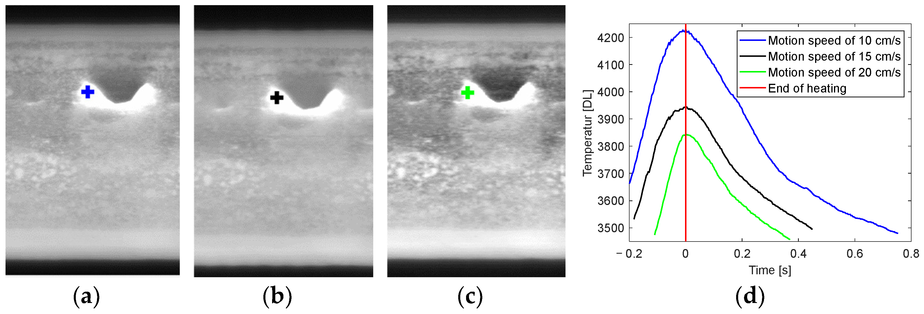
Temperature increases and motion speed:Figure 17 compares the temperature increase in the case of three different motion speeds, determined for the position close to the defect, after reordering the recorded IR sequence. The temperature increase due to the inductive heating is affected by the motion speed through the heating region of the inductor. Slower speed causes a longer excitation period and, therefore, higher temperature increase. In the transformed quasi stationary sequence, it can be observed that temperature curves look similar to that of stationary pulse measurements. The duration of these pseudo-pulses can be approximated by the time of how long the specimen needs to go through the effective heating range underneath the inductor. For motion speeds of 100, 150 and 200 mm/s and an effective heating range of inductor with a width of 20 mm, this results in pulse durations of approximately 0.1, 0.15 and 0.2 s, respectively (see Figure 17d).

II.

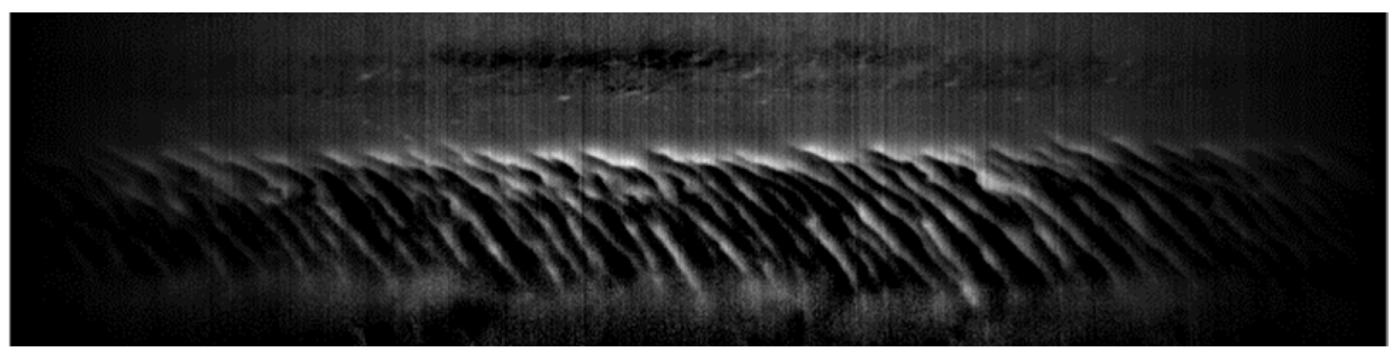
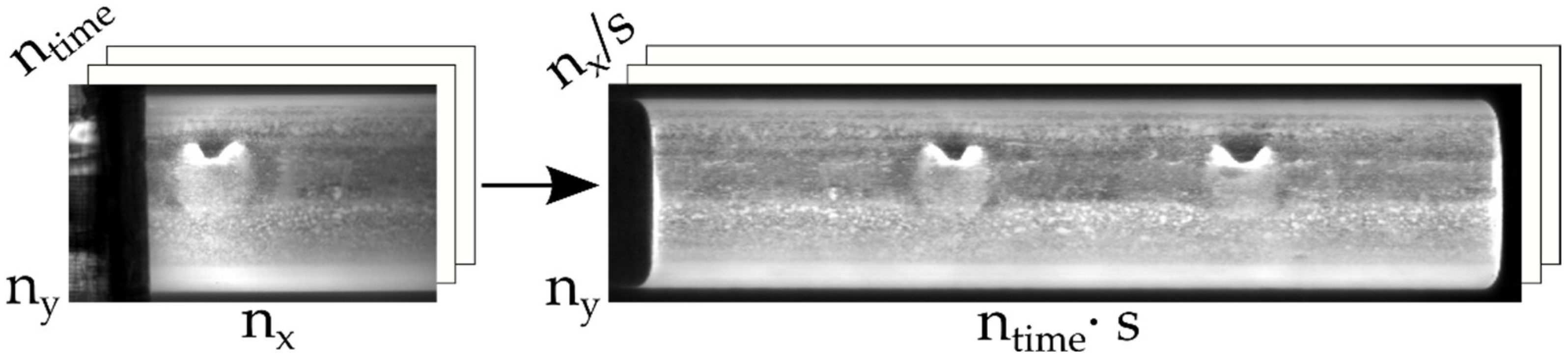
Camera frame rate and image resolution: As described in [11], during the transformation to the quasi stationary sequence, the size of the images and the number of the frames are changed. The new image size in motion direction x is determined by the pixel columns running through the entire camera’s FOV. This can be calculated by multiplying the number of frames in the original sequence and the shift s, as in Figure 18. However, if the shift s significantly deviates from an ideal shift of 1 px, this calculation is inaccurate due to interpolation during the transformation. Therefore, through this transformation, the camera’s frame rate impacts the spatial resolution of the transformed images. The number of frames in the transformed sequence is the quotient of n_x, the number of pixels in motion direction in the original sequence and the shift s (see Figure 18). This means that the spatial resolution of the original image affects the temporal resolution of the created sequence.

III.

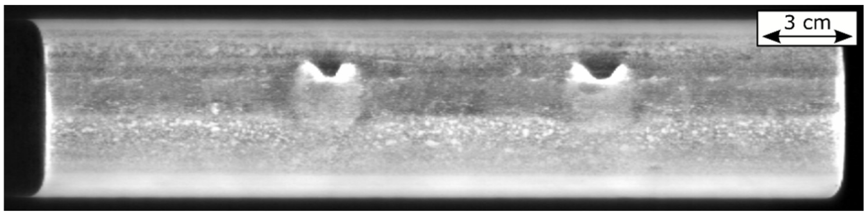
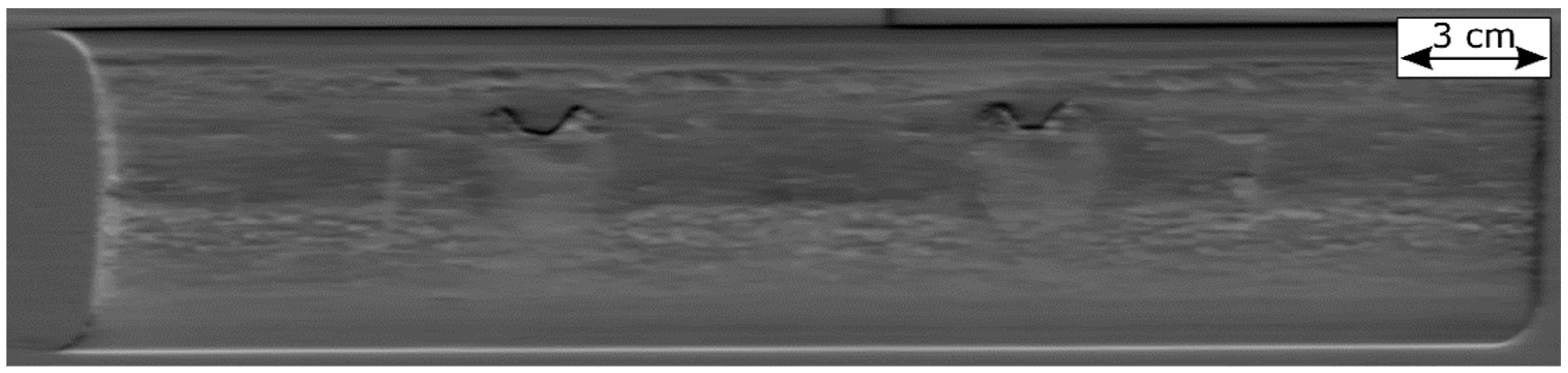
Evaluation with phase image: For the calculation of the phase with Fourier transform, the images recorded during the heating pulse and afterwards during the cool-down are used. The following question arises: how many images during the cool- down should be considered? Earlier works show [7] that for phase images, the relationship between pulse length and cool-down-period influences the result. For stationary measurements, often a cool-down-period with the same length as the heating pulse itself is chosen. As described in point II for scanning, this is not so much a temporal length as it is rather a spatial length. This means that the recorded area underneath the inductor resembles the pulse length and the recorded area behind the inductor resembles the cool-down-period. In the case of the measurement in Figure 16, a distance of 45 mm in the moving direction was covert by the camera’s FOV, from this 15 mm underneath the inductor and 30 mm behind the inductor. Therefore, the resulting phase image is an evaluation of a certain pulse length and additionally a cool-down-period, which is two times longer than the pulse length. Since the FOV needed for phase evaluation is rather small, it is possible to reduce the camera’s image size in y-direction, which further allows for higher frame rates and, thus, increasing the resolution of the result.

All the described parameters are interdependent. The frame rate of the used camera speed is an important factor to change and test different parameter settings. Future research will discuss the detectability of small surface defects with this modified SPPT method with a focus on the three described parameters. Cooled camera systems with high resolution and high frame rates are, of course, beneficial for this type of testing; however, uncooled systems with higher frame rates show also high potential for such scanning applications and are more suitable for mobile inspection setups. Figure 19 shows that a moving speed of 150 mm/s still provided a decent result with a high speed uncooled camera system.

References

1. Oswald-Tranta, B. Induction thermography for surface crack detection and depth determination. Appl. Sci. 2018, 8, 257. [Google Scholar] [CrossRef] [Green Version]
2. Maldague, X. Infrared and thermal testing. In Nondestructive Testing Handbook; ASNT: Columbus, OH, USA, 2001; Volume 3. [Google Scholar]
3. Netzelmann, U.; Walle, G.; Lugin, S.; Ehlen, A.; Bessert, S.; Valeske, B. Induction thermography: Principle, applications and first steps towards standardisation. Quant. Infrared Thermogr. J. 2016, 13, 170–181. [Google Scholar] [CrossRef]
4. Vrana, J.; Goldammer, M.; Baumann, J.; Rothenfusser, M.; Arnold, W. Mechanism and models for crack detection with induction thermography. AIP Conf. Proc. 2008, 975, 475–482. [Google Scholar] [CrossRef]
5. Srajbr, C. Induction excited thermography in industrial applications. In Proceedings of the 19th World Conference on Non-Destructive Testing, Munich, Germany, 13–17 June 2016. [Google Scholar]
6. DIN 54183:2018-02; Non-Destructive Testing-Thermographic Testing-Eddy-Current Excited Thermography. Deutsches Institut für Normung: Berlin, Germany, 2018. Available online: https://www.din.de (accessed on 1 January 2018).
7. Oswald-Tranta, B. Time-resolved evaluation of inductive pulse heating measurements. Quant. InfraRed Thermogr. J. 2009, 6, 3–19. [Google Scholar] [CrossRef]
8. Ahmadi, S.; Burgholzer, P.; Jung, P.; Caire, G.; Ziegler, M. Super resolution laser line scanning thermography. Opt. Lasers Eng. 2020, 134, 106279. [Google Scholar] [CrossRef]
9. Tuschl, C.; Oswald-Tranta, B.; Eck, S. Inductive Thermography as Non-Destructive Testing for Railway Rails. Appl. Sci. 2021, 11, 1003. [Google Scholar] [CrossRef]
10. Lehtiniemi, R.; Hartikainen, J. An application of induction heating for fast thermal nondestructive evaluation. Rev. Sci. Instrum. 1994, 65, 2099–2101. [Google Scholar] [CrossRef]
11. Oswald-Tranta, B.; Sorger, M. Scanning pulse phase thermography with line heating. Quant. InfraRed Thermogr. J. 2012, 9, 103–122. [Google Scholar] [CrossRef]
12. Peeters, J.; Verspeek, S.; Sels, S.; Bogaerts, B.; Steenackers, G. Optimized dynamic line scanning thermography for aircraft structures. Quant. InfraRed Thermogr. J. 2019, 16, 260–275. [Google Scholar] [CrossRef]
13. Chulkov, A.O.; Tuschl, C.; Nesteruk, D.A.; Oswald-Tranta, B.; Vavilov, V.P.; Kuimova, M.V. The Detection and Characterization of Defects in Metal/Non-metal Sandwich Structures by Thermal NDT, and a Comparison of Areal Heating and Scanned Linear Heating by Optical and Inductive Methods. J. Nondestruct. Eval. 2021, 40, 44. [Google Scholar] [CrossRef]
14. 2-D Polynomial Geometric Transformation—MATLAB—MathWorks Deutschland. Available online: https://de.mathworks.com/help/images/ref/images.geotrans.polynomialtransformation2d.html (accessed on 4 April 2022).
15. Oswald-Tranta, B. Temperature reconstruction of infrared images with motion deblurring. J. Sens. Sens. Syst. 2018, 7, 13–20. [Google Scholar] [CrossRef] [Green Version]
Figure 1. (a) A 250 mm long rail piece with head checks (RP01); (b) detailed view of the head checks on the gauge corner; area with head checks marked in red.
Applsci 12 05851 g001
Figure 2. (a) A 300 mm rail piece with squats (RP02); (b) detailed picture of a large squat on the specimen; area with squats marked in red.
Applsci 12 05851 g002
Figure 3. (a) Setup for scanning in a stop-and-go technique; (b) setup for continuous scanning.
Applsci 12 05851 g003
Figure 4. (a) Paper grid wrapped around a rail piece; (b) calibration image of the paper grid recorded by the IR camera; (c) metallic grid on top of a rail piece; (d) IR calibration image of the metallic grid.
Applsci 12 05851 g004
Figure 5. (a) Calibration image as it is recorded with the IR camera; (b) binary checkerboard grid with detected checkerboard corner points marked in red; (c) equidistant quadratic grid, obtained after the calculated transformation and used on the calibration image (a).
Applsci 12 05851 g005
Figure 6. (a) Recorded phase image of a segment of the gauge corner; (b) phase image after rectification transformation is applied; (c) cropped segment of the transformed phase image.
Applsci 12 05851 g006
Figure 7. (a) Overlapping of two consecutive phase images with marked region of interest for phase correlation; (b) shift of the second image according to the result of the phase correlation.
Applsci 12 05851 g007
Figure 8. Phase image with fading in (0–100%) of pixel values on the left and fading out (100–0%) of pixel values on the right side.
Applsci 12 05851 g008
Figure 9. Panoramic phase image computed from five measurements for a whole length of 250 mm.
Applsci 12 05851 g009
Figure 10. Postprocessing of measurements in continuous motion.
Applsci 12 05851 g010
Figure 11. (a) IR image of the squat defect during scanning, inductor is visible on the left side; (b) image after applied rectification transformation.
Applsci 12 05851 g011
Figure 12. Temperature image of the specimen after re-organizing the pixel-columns.
Applsci 12 05851 g012
Figure 13. Resulting phase image of a measurement with a scanning speed of 200 mm/s.
Applsci 12 05851 g013
Figure 14. Comparison of cracks detected with scanning (left image) and cracks detected with stationary measurement (right image).
Applsci 12 05851 g014
Figure 15. Resulting phase image of a measurement taken with a µ-bolometer camera and a scanning speed of 50 mm/s.
Applsci 12 05851 g015
Figure 16. Measurement with µ-bolometer camera and increased frame rate (100 Hz) with a scanning speed of 50 mm/s.
Applsci 12 05851 g016
Figure 17. Evaluation of points in the transformed image for measurements with (a) 100 mm/s; (b) 150 mm/s; (c) 200 mm/s; (d) time vs. temperature graph of the three evaluated points.
Applsci 12 05851 g017
Figure 18. Scheme of conversion of rectified nx × ny × ntime sequence to quasi static ntime·s × ny× nx/s image sequence.
Applsci 12 05851 g018
Figure 19. Measurement with µ-bolometer camera and increased frame rate (200 Hz) with a scanning speed of 150 mm/s.
Applsci 12 05851 g019