Transfer Learning Analysis for Subvisible Particle Flow Imaging of Pharmaceutical Formulations

Abstract

Subvisible particles are an ongoing problem in biotherapeutic injectable pharmaceutical formulations, and their identification is an important prerequisite for tracing them back to their source and optimizing the process. Flow imaging microscopy (FIM) is a favored imaging technique, mainly because of its ability to achieve rapid batch imaging of subvisible particles in solution with excellent imaging quality. This study used VGG16 after transfer learning to identify subvisible particle images acquired using FlowCam. We manually prepared standards for seven classes of particles, acquired the image information through FlowCam, and fed the images over 5 µm into VGG16 consisting of a convolutional base of VGG16 pre-trained with ImageNet data and a custom classifier for training. An accuracy of 97.51% was obtained for the test set data. The study also demonstrated that the recognition method using transfer learning outperforms machine learning methods based on morphological parameters in terms of accuracy, and has a significant training speed advantage over scratch-trained CNN. The combination of transfer learning and FIM images is expected to provide a general and accurate data-analysis method for identifying subvisible particles.

1. Introduction

Therapeutic protein formulations are among the fastest-developing pharmaceutical classes. Pharmaceutical formulations always contain subvisible particles owing to the limitations of the production process and the instability of the proteins [1]. According to the discussion in USP1790 [2], particles in protein formulations can usually be classified as “extrinsic”, “intrinsic”, or “inherent” particles. Extrinsic particles can be considered foreign to the manufacturing process, including hair, non-process-related fibers, starch, minerals, and similar inorganic and organic materials. Intrinsic particles are those related to the manufacturing process, which may originate from processing equipment or packaging materials, including seals, gaskets, packaging glass and elastomers, fluid transport tubing, and silicone lubricant. Inherent particles are associated with the production formulations and primarily contain protein aggregates. Protein aggregation mainly results from changes in product stability caused by stress in industrial production, including freeze–thawing, mechanism shock, shaking and shearing, elevated temperatures, oxidation, or a combination of these stresses [3,4,5,6]. Because particles may cause sterile failure or even produce severe immunogenic reactions [7,8,9], endangering patient safety [10], the FDA and other regulatory agencies have imposed strict quantitative limits on protein aggregates and other particles in pharmaceutical formulations. USP<788> [11] requires pharmaceutical formulation product manufacturing departments to monitor particle content using light obscuration or microscopy, and to set a firm upper limit for the number of particles above 10 μm and 25 μm to ensure that the formulation is free of particles. Because of the complexity of the sources of particles and their possible adverse effects, it is imperative to identify the particles, which helps to trace their sources and thus avoid them in the manufacturing process, thereby reducing the potential risk of adverse reactions caused by these particles at the source.

Over the past few years, flow imaging microscopy (FIM) has been widely used as an increasingly popular imaging technology in cutting-edge research in environmental science, biology, pharmacology, and other disciplines. This is mainly because FIM instruments, such as FIM or FlowCam, can image particles/microorganisms between 2 µm and 200 µm in diameter in rapid batches [12] and obtain high-quality images. FlowCam consists of a 10× microscope, camera, software, and flow cell with a flow rate controlled by a vacuum pump. After injecting the liquid, the liquid flows through the flow cell at a low speed under the action of the pump, while the camera captures images at a high framerate. Additionally, the software extracts independent particle images from the camera images through threshold extractions. Such an FIM instrument can perform particle counting and provide more than 1000 single-particle images with a large number of morphological features in each experiment.

Because of the difference in imaging principles, FIM is more sensitive than the light obscuration method in counting translucent particles [13], such as protein particles, and has been increasingly used to monitor the particle content in protein preparations. USP<1788> [14] even introduced a revised chapter using FIM to support light obscuration and microscopy methods for determining subvisible particles. However, most studies using FIM have focused on analyzing particle concentration or simple particle parameters. For example, FIM is used to determine the relationship between the stress type and particle quantity [15], or identify simple morphological features to distinguish between protein and silicone oil [16]. However, using simple morphological features extracted by image-based algorithms often leads to the loss of a great deal of information in the complete grayscale image provided by FIM.

Convolutional neural networks (CNNs) are believed to learn the optimal features that can be used to automatically characterize an image from the original image [17]. CNNs have advanced the analysis of macroscopic image classifications. With supervised learning and massive image datasets, CNNs have revolutionized many practical applications of image analysis. In recent years, the accuracy of automatic image classification based on CNNs has improved with the advancement of algorithms, the performance of graphics processors, and the proliferation of datasets in various fields [18]. In some application scenarios, such as breast cancer identification [19], the performance of CNNs has matched or even surpassed that of human eye recognition. These advances have enabled efficient and robust construction of deep CNNs with multiple implicit layers. Deep CNNs can use large amounts of data to learn the optimal features automatically to characterize an image in each classification task. This approach makes complete use of image grayscale information compared to using conventional morphological features.

FIM combined with CNN research has also been increasingly popular in recent years. CNN has not only obtained excellent classification results in plankton above 50 microns in size [20], but also showed potential in the subvisible particles of pharmaceutical formulations. Current research has focused on the classification of protein particle stress sources [21,22] and the classification between proteins and silicone oils [23,24], while ignoring other extrinsic and intrinsic particles that may also cause negative effects. Our study achieves the classification of seven classes of particles, which comprise inherent, extrinsic and intrinsic particles. This demonstrates the feasibility of FIM combined with CNN methods to achieve particle classification among multiple materials and types.

In addition, because of the heterogeneity of protein particles, protein stress classification often relies on complex feature extraction methods or classification strategies, and thus it is not conducive for use in varied real process conditions. In contrast, the features learned from the ImageNet dataset can be regarded as a generic model for the visual world and applied in various fields, regardless of whether the task is relevant to ImageNet’s or not [25]. This study uses an ImageNet-pre-trained convolutional base plus a custom classifier for transfer learning, and the features learned from ImageNet can be applied to particle classification after fine-tuning of the classifier. Unlike the deep learning methods in other studies, the transfer learning used in this study converges faster, requires a smaller dataset, and does not require feature extraction from scratch. Therefore, transfer learning is expected to be applied as a simple, fast and general method for subvisible particle classification in real process conditions.

This study proposes a pre-trained CNN-based particle classification method to identify subvisible particles (5–80 µm) commonly found in pharmaceutical protein formulations containing protein particles, cap fiber particles, glass particles, silicone oil microdroplets, silicone tubing particles, rubber closure particles, and polystyrene beads. Specifically, we prepared seven classes of standard particles of different sizes, imaged the standard samples in combination with FlowCam, then segmented and resized the images. The image set was used as the dataset of the neural network, which was then trained and validated on ImageNet-pre-trained VGG-16 to differentiate the seven classes of particles. This study demonstrates the potential of CNNs in classifying pharmaceutical formulation particles at the single-particle image level to achieve the traceability of particles.

2. Materials and Methods

2.1. Sample Preparation

Seven standard particle samples, including protein, cap fiber, glass, silicone oil microdroplets, silicone tubing, rubber closure, and polystyrene beads, were prepared and used for CNN classification. Among them, cap fiber particles are considered extrinsic and originate from bouffant caps in the production environment. Glass particles, silicone oil microdroplets, silicone tubing particles, and rubber closure particles are considered intrinsic particles originating from the materials that may encounter the process. Protein particles are inherent. Polystyrene beads were used as the focus beads for the FlowCam.

Cap fibers, silicone tubing, rubber closure particles, and glass particles were prepared using a stainless-steel shredder (FSJ-A03D1, Bear, Foshan, China) separately from the raw material of the spunbonded polypropylene fabric from bouffant caps (I113-1459) (VWR, Atlanta, GA, USA). We purchased 1.5 mL PP microcentrifuge tubes (509-GRD-Q) from Quality Scientific Plastics (Petaluma, CA, USA), 20 mm rubber closures (V10-F597W RS) from Daikyo Seiko, Ltd. (Tochigi, Japan), and 30 mL Fiolax clear vials (39214A) from SCHOTT Vials (Müllheim, Germany). After each class of particle was collected, subvisible particles below 100 µm in diameter were filtered through a 100 µm pore-size nylon cell strainer (93100, SPL Life Sciences, Pocheon-si, Korea) and diluted in purified water to form the corresponding particle solution. The same process was performed with pure water as the control to ensure that no new particles were introduced into the filtration process. The silicone oil particle solution was diluted from silicone oil (PMX-200; Aladdin, Shanghai, China) with purified water (1:1000) and sonicated for 3 min. Polystyrene beads were purchased from Micro Measurement Labs (Wheeling, WV, USA), with 3000 25 µm-diameter polystyrene beads per milliliter.

In this study, protein particles were prepared by simulating shaking-induced stress. IgG1 antibody (Mab1) formulation solution (25 mg/mL protein in formulation buffer, pH 6.2) was donated by a local biopharmaceutical company. To generate protein particles, the solution was dispensed into five vials and stirred at 400 rpm for 1 h using a magnetic stirrer (YYCJ-35, Yuyong Biotechnology, Shanghai, China).

2.2. FlowCam Imaging

Images were acquired with a FlowCam^® 8100 (Fluid Imaging Technologies, Inc., Scarborough, Scarborough, ME, USA) equipped with a 1600 µm-long, 800 µm-wide, and 80 µm-deep flow cell with a 10× objective for image acquisition. For each sample, 1 mL of the particulate sample was added; the sample flow rate was 0.5 mL/min and the camera frame rate was 90 fps, and this was repeated 1–5 times depending on the particulate concentration. Before the experiment started, and every time the sample was switched, the flow cell was washed once with the FlowCam special washing solution and then five times with Milli-Q water, after which the flow cell was verified for residual particles with pure water. All images were initially screened using the VisualSpreedsheet^® program for equivalent spherical diameter (ESD) > 5 μm and edge gradient > 20 to filter out misidentified and small particles.

2.3. Data Analyses

2.3.1. Image Preprocessing

All acquired images were first cropped along the black border in MATLAB to obtain individual particle images and were numbered by category. Data cropping was performed using MATLAB R2019b (MathWorks, Natick, MA, USA).

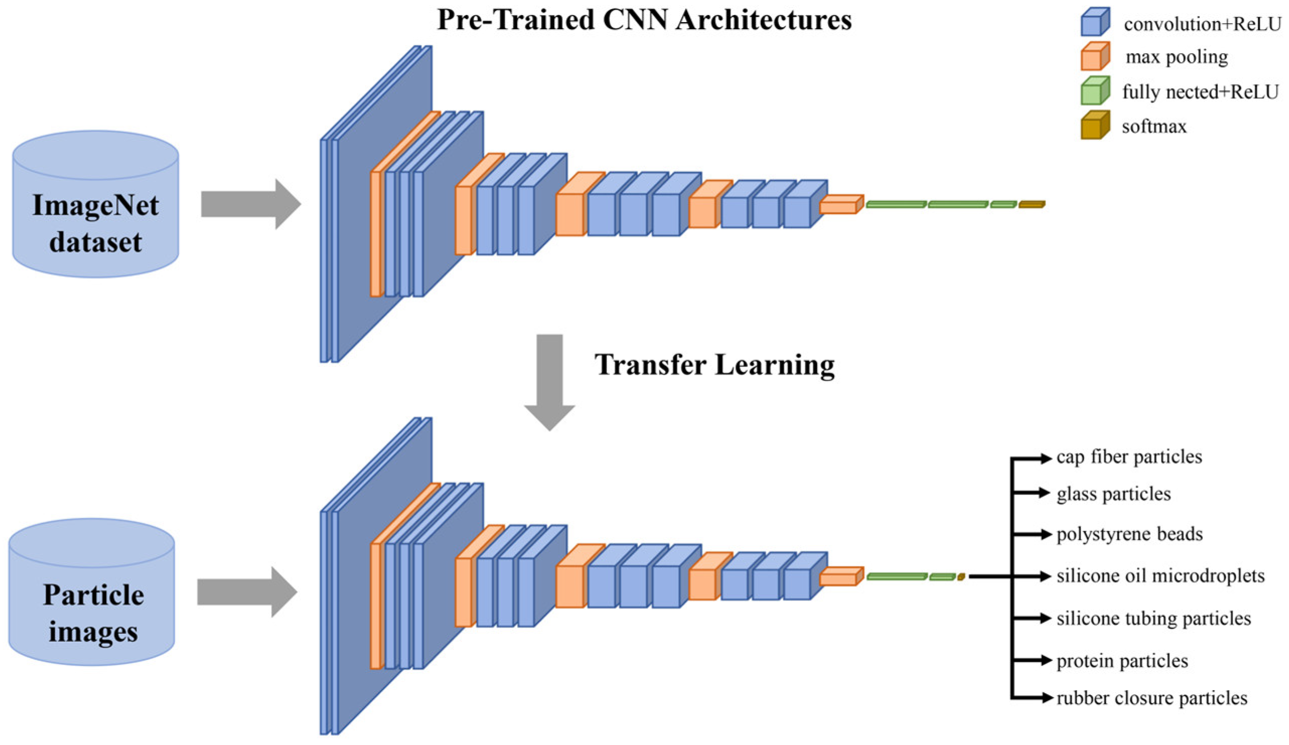
2.3.2. Convolutional Neural Networks

Our work focused on classifying seven classes of particles by training VGG16 pre-trained on ImageNet. VGG16 [26] was developed by Karen Simonyan and Andrew Zisserman from the Visual Geometry Group (VGG) at the University of Oxford, and won first place in the 2014 ILSVRC object-recognition challenge. Its main objective is to improve the depth of the neural network while following the basic structure of AlexNet to achieve better performance. Specifically, it uses several consecutive 3 × 3 convolutional kernels instead of the larger convolutional kernels (11 × 11, 7 × 7, and 5 × 5) used in AlexNet, as more convolutional layers can help to extract more abstract higher-order features with fewer parameters.

The structure of a CNN consists of three parts: a convolutional layer, a pooling layer, and a fully connected layer. For convolution, after the image is input as a matrix into the CNN, the image matrix is passed through various filters to generate different feature maps, thereby obtaining different image features. For example, the filters of the first convolutional layer typically correspond to the edge and color block information of the image. As the input of each convolutional layer is the output of the previous convolutional layer, filters located deeper in the network can extract more complex morphological features and increasingly abstract visual concepts. The purpose of the pooling layer is to downsample the feature maps, which can reduce the number of elements in the maps to be processed and allow successive convolutional layers to have increasingly larger observation windows, thereby introducing a hierarchical structure of spatial filters. The fully connected layer plays the role of a classifier in the CNN, where the representatives of the convolutional and pooling layers map the input image to the feature space, and the fully connected layer maps these features to the sample-labeling space. The VGG16 used in this study contained 13 convolutional layers, 5 max-pooling layers, and 3 fully connected layers. Alternatively, it consisted of a convolution base with a classifier.

During training, the CNN took the images in the training set as the input and obtained the probability of the images corresponding to each category through the forward propagation process. It then obtained the loss function value of the output layer according to the image labels, calculated the gradient of the error on each weight in the network using back propagation, and updated the values/weights of all filters using the gradient descent method to minimize the loss function value. This process was repeated during training. After training, the network classified images that were not included.

This study used two methods to train the CNN. The first used VGG16 pre-trained on ILSVRC-2012, a subset of ImageNet, which is a large dataset containing 1.4 million labeled images with 1000 different classes. The data size of this dataset is sufficiently large and general and usually represents natural images. As shown in Figure 1, we used the pre-trained convolutional base of VGG16 (containing 13 convolutional layers and 5 max-pooling layers) with a final feature map shape of 4 × 4 × 512. We added a three-layer densely connected classifier to this feature to match our particle classification requirements. We froze the parameters in the convolutional base during training, and trained only the classifier. One main advantage of using transfer learning is that it trains only a small part of the network, resulting in a faster learning process than that of training the entire network. This reduces the risk of overfitting by reducing many training parameters, and smaller datasets can be used for transfer learning, avoiding the risk of overfitting by directly training small datasets. In another approach, we used the same network structure, but initialized all layers with random parameters and did not freeze any layers, thus training a CNN from scratch.

A total of 9500 images of each labeled particle class were used as a training set to train the network to predict the particle class. Two thousand images of each labeled particle class were used as a validation set to tune the parameters of the classifier. Additionally, 2000 images of each labeled particle class were used as a test set to assess the performance of the classifier. The particle images were resized to 150 × 150 pixels and normalized in terms of intensity before entering the network.

Table 1. CNN structure used in this study.

Lay No.	Layer Type	No. of Features	Feature Size	Activation	Input Shape	Output Shape
1	Convolutional	64	3 × 3	ReLU	150 × 150 × 3	150 × 150 × 64
2	Convolutional	64	3 × 3	ReLU	150 × 150 × 64	150 × 150 × 64
3	Max pooling (2 × 2)	–	–	–	150 × 150 × 64	75 × 75 × 64
4	Convolutional	128	3 × 3	ReLU	75 × 75 × 64	75 × 75 × 128
5	Convolutional	128	3 × 3	ReLU	75 × 75 × 128	75 × 75 × 128
6	Max pooling (2 × 2)	–	–	–	75 × 75 × 128	37 × 37 × 128
7	Convolutional	256	3 × 3	ReLU	37 × 37 × 128	37 × 37 × 256
8	Convolutional	256	3 × 3	ReLU	37 × 37 × 256	37 × 37 × 256
9	Convolutional	256	3 × 3	ReLU	37 × 37 × 256	37 × 37 × 256
10	Max pooling (2 × 2)	–	–	–	37 × 37 × 256	18 × 18 × 256
11	Convolutional	512	3 × 3	ReLU	18 × 18 × 256	18 × 18 × 512
12	Convolutional	512	3 × 3	ReLU	18 × 18 × 512	18 × 18 × 512
13	Convolutional	512	3 × 3	ReLU	18 × 18 × 512	18 × 18 × 512
14	Max pooling (2 × 2)	–	–	–	18 × 18 × 512	9 × 9 × 512
15	Convolutional	512	3 × 3	ReLU	9 × 9 × 512	9 × 9 × 512
16	Convolutional	512	3 × 3	ReLU	9 × 9 × 512	9 × 9 × 512
17	Convolutional	512	3 × 3	ReLU	9 × 9 × 512	9 × 9 × 512
18	Max pooling (2 × 2)	–	–	–	9 × 9 × 512	4 × 4 × 512
19	Flatten	–	–	–	4 × 4 × 512	8192
20	Dense	1024	n/a	ReLU	8192	1024
21	Dropout (50% rate)	–	–	–	1024	1024
22	Dense	512	n/a	ReLU	1024	512
21	Dropout (30% rate)	–	–	–	512	512
22	Dense	7	n/a	Softmax	512	7

ReLU, rectified linear unit.

shows the specific structure of the network, which added three custom fully connected layers to the traditional VGG16 convolutional base, contained a total of 23.63 million parameters, and used categorical cross-entropy as the loss function, RMSprop as the optimizer, and accuracy as the metrics. The networks were trained for 100 epochs, and the batch size was 128. All layers were implemented in Keras 2.3.1 (TensorFlow 1.14.0 backend). The calculations were performed using Windows 10 on an NVIDIA GeForce GTX 2070 machine.

2.3.3. Machine Learning

In this study, we used a machine-learning-based approach for particle classification. First, we used the canny function in OpenCV to obtain the profile of each particle and its 15 morphological parameters: length, width, perimeter, area, filled area, circularity, circularity (Hu), intensity, sigma intensity, roughness, compactness, Sobel gradient, and Laplacian gradient. A total of 13,000 images per class of particle, for a total of 91,000 × 15 data points, were used to perform five machine learning algorithms for classification: decision trees, linear discriminants, support vector machines, nearest neighbor classifiers, and ensemble classifiers, which were trained using the 10-fold cross-validation method. Single-particle contour and feature extraction was performed using OpenCV 3.4.2, whereas machine learning classification was performed using the Classification Learner App in MATLAB R2019b (MathWorks).

3. Results and Discussion

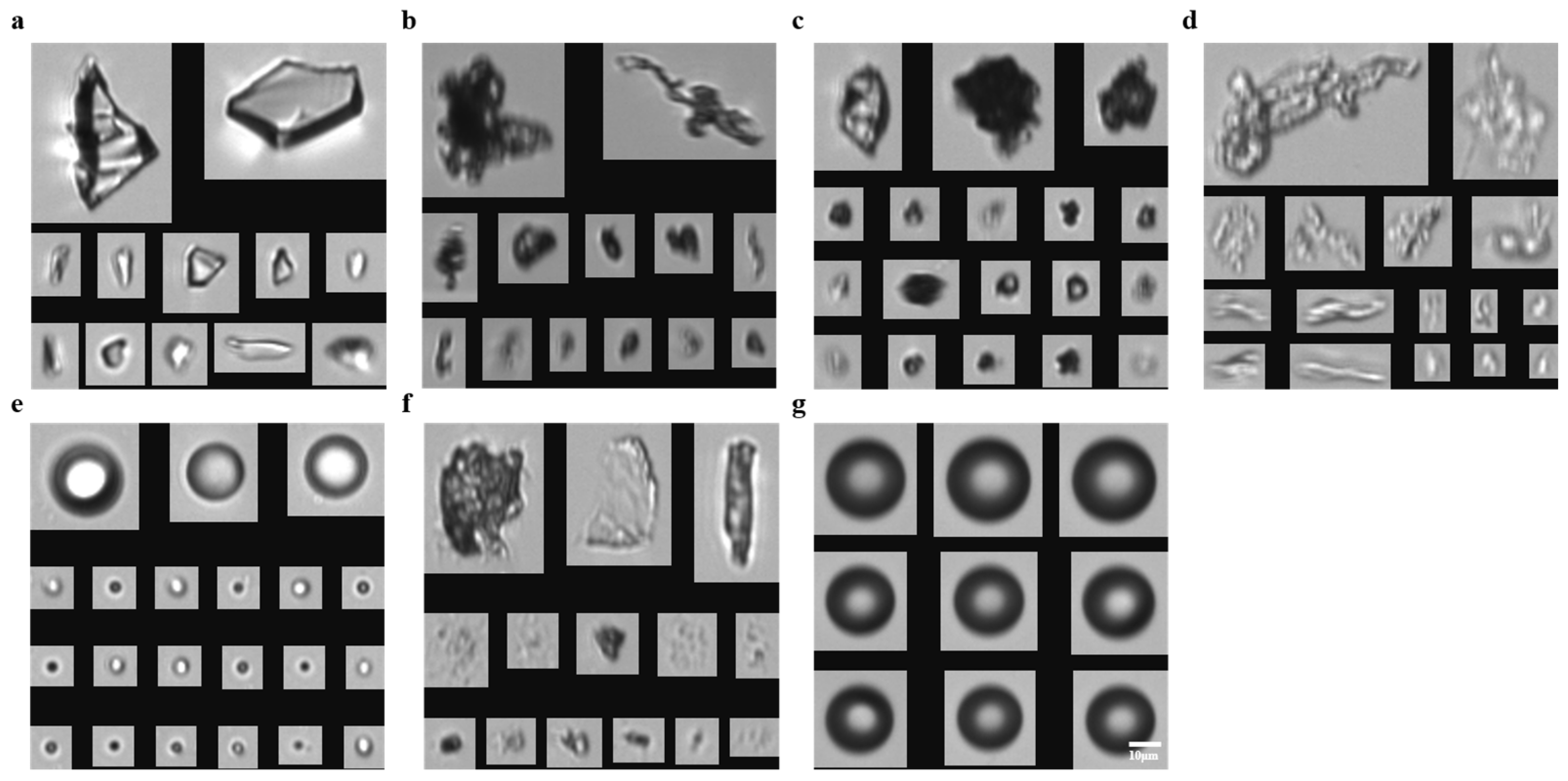
3.1. Particle FIM Imaging

Sample FIM images of seven classes of particles are shown in Figure 2. Glass is one of the most commonly used containers in injectable pharmaceutical processes. Glass particles are mainly formed because of the breakage of glass vials during filling or subsequent storage and transportation. In the glass particle solution prepared from the vial, the most noticeable characteristics of the glass particles (Figure 2a) are their relatively sharp edges and their translucent nature. Cap fibers are derived from bouffant caps, which are typically extrinsic particles that may be introduced into the filled drug product solution through environmental contamination during gowning and filling operations. Particle images (Figure 2b) show that the cap fibers were primarily a flexible combination of long strips which are partly transparent. The rubber closures matched the glass vials used to seal them. These particles enter the pharmaceutical formulation primarily during the filling process or during subsequent preservation and transportation. The image of the rubber closure particles prepared by crushing the rubber closures (Figure 2c) shows black, irregularly shaped opaque blocks with flocculent-like edges. Protein aggregation is a major source of particles in pharmaceutical formulations. Protein particles may originate from a variety of processes in the manufacturing of pharmaceutical products, such as unexpected high-temperature exposure during production, shear stress during the freeze–thaw process of drug substances, the mixing of compounded bulk drug products, bulk transfer via a peristaltic pump or gas pressure, filtration, and filling. The protein particles were prepared by simulating shaking stress in a magnetic shaker, and the most notable features of the protein particles (Figure 2d) were their translucency and diverse morphologies. Silicone oil is commonly used as a lubricant in various containers (e.g., vials, pre-filled syringes, cartridges, and plungers). Silicone oil microdroplets may appear in pharmaceutical formulations because of the leachability of these container surfaces. Figure 2e shows distinctly spherical microdroplets with translucent centers. Silicone tubing is commonly used for solution transport and solution filling, and may form silicone tubing granules due to flaking during transport. The silicone tubing particles formed by crushing (Figure 2f) were irregular blocks, either translucent or opaque.

As shown in the images, each of the six particles displayed more than two different morphologies. For example, silicone oil had two morphologies: a bright center within a dark circle, and a dark center within a bright white ring. This is due to the depth of field of the 10× lens (approximately 10 μm) being much smaller than the depth of the flow cell (80 μm). According to the working principle description, based on hydrodynamic action, particles tend to move downwards along two cross-sections within the flow cell; approximately half of the particles are not in the focal plane, which is one of the most important sources of image diversity of the same particles. The FlowCam images of the polystyrene beads (Figure 2g) show black spheres with white centers. In this study, these beads were extracted only in the focal plane because of their limited practical significance, and were mainly used as a standard particle reference to demonstrate the feasibility of the CNN model. Polystyrene beads were used as standard particles for FlowCam to adjust the focus as a reference in the flow cell.

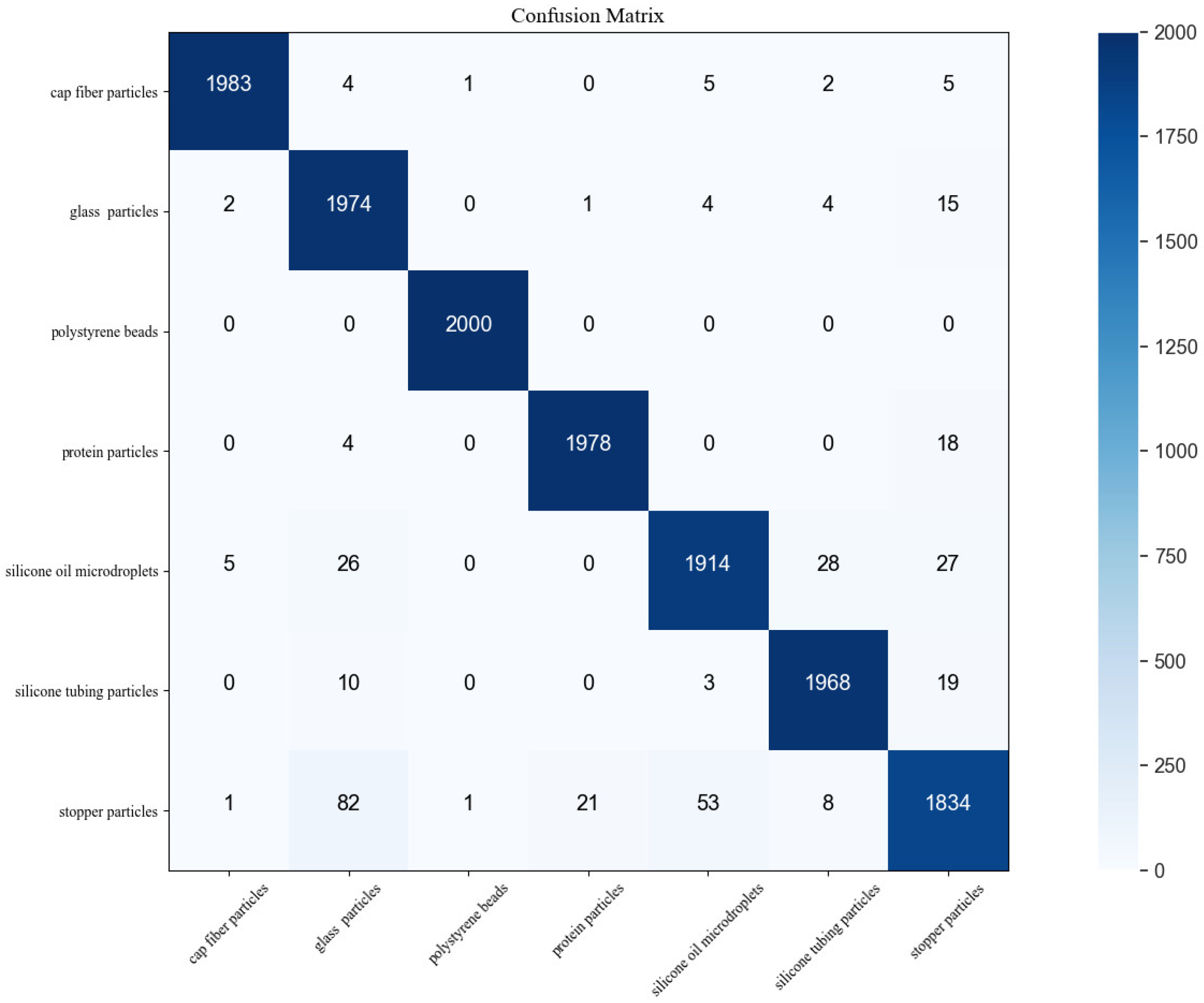
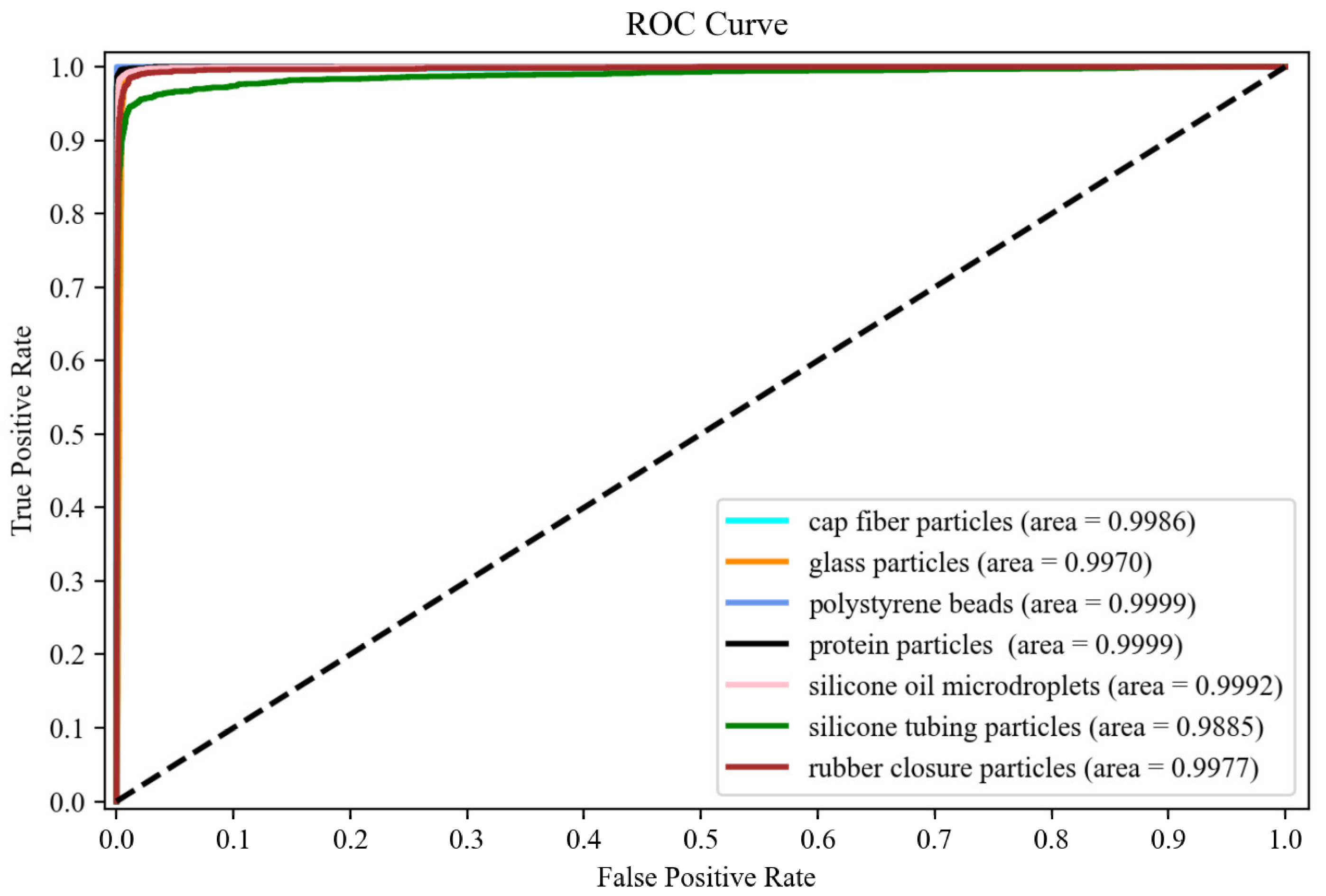
3.2. CNN Transfer Learning for Subvisible Particle Classification

To classify pharmaceutical formulation particles, we fine-tuned the VGG16 network based on the ImageNet dataset. For a total of 2000 × 7 test set samples, the classification efficiency of this CNN classifier was 97.51% for seven different particles and 97.09% after excluding polystyrene standard particles. Using the confusion matrix (Figure 3), different metrics can be derived to indicate the classifier’s performance, specifically for each class of particle; the accuracy of protein particles, cap fiber particles, glass particles, silicone oil microdroplets, and polystyrene beads was above 98%. The relative recognition rates of the silicone tubes and rubber particles were lower (91.70% and 95.70%, respectively). It is possible that the silicone tube particles were recognized as glass, protein, and rubber closure particles, and the rubber closure particles were misidentified as glass, silicone oil, and silicone tube particles. This may be related to the morphological diversity of granules at low sizes. The results show that by using the VGG16 architecture based on ImageNet pre-training, after transfer learning to train the fully connected layer, it is possible to achieve over 97% accurate recognitions of individual particles of different types. On the contrary, it is difficult for humans to make accurate subjective classifications directly from individual particle images. CNNs can achieve composition recognition of particles based on individual grayscale particle images, which in turn helps to trace the sources of particles under production conditions, optimize the sources in a targeted manner, improve the production process, and prevent exogenous particles from entering pharmaceutical formulations at the source.

To evaluate the generalization ability of the model, we introduced precision, recall, F-score, and a receiver operating characteristic (ROC) curve in addition to accuracy. The precision for a class is the number of true positives divided by the total number of elements labeled as belonging to the positive class. In this context, recall is defined as the number of true positives divided by the total number of elements that actually belong to the positive class. These are defined as follows:

$$precision=\frac{TP}{TP+FP}$$

(1)

$$recall=\frac{TP}{TP+FN}$$

(2)

where TP, FP, TN, and FN are defined as true positive, false positive, true negative, and false negative, respectively. The F-score is a composite of recall and precision and is the harmonic mean of the two, as defined below:

$$F=2 \frac{precision·recall}{precision+recall}$$

(3)

The ROC curve is a graph showing the performance of the classification model at all classification thresholds. The curve consists of two parameters: the true positive rate (TPR) in the vertical coordinate, and the false positive rate (FPR) in the horizontal coordinate. TPR is equal to the recall rate; TPR and FPR are defined below. The area under the curve (AUC) is typically used to assess the ROC curve, and provides an aggregate measure of performance across all possible classification thresholds. The AUC is scale-invariant and classification threshold-invariant. The AUC ranges from 0 to 1; generally, the closer the AUC is to 1, the higher the accuracy of the classifier.

$$TPR=\frac{TP}{TP+FN}$$

(4)

$$FPR=\frac{FP}{FP+TN}$$

(5)

When considering one class of particles, the accuracy can be considered the same as the recall rate; accuracy-related conclusions have been mentioned previously.

Table 2. Recall, precision, and F-score evaluation of particle classification.

Particle Type	Precision	Recall	F-Score
Cap fiber particles	99.60%	99.15%	99.37%
Glass particles	94.00%	98.70%	96.29%
Polystyrene beads	99.90%	100.00%	99.95%
Protein particles	98.90%	98.90%	98.90%
Silicone oil microdroplets	97.91%	98.40%	98.15%
Silicone tubing particles	95.62%	91.70%	93.62%
Rubber closure particles	96.72%	95.70%	96.21%

lists the precision, recall, and F-scores of each particle. All particles showed high precision rates of 94% and above. Similar conclusions were obtained when the F-score was used to measure recall and precision, with a total combined F-score of 97.50% and scores above 93.50% for each particle class.

The ROC curve and the corresponding AUC are shown in Figure 4. The findings show a very steep cliff pattern in the ROC curve, with an AUC above 0.9885 for seven classes of particles. Taken together, the recall, accuracy, ROC curve, and AUC confirm the usability of the model, avoiding problems that may arise from assessing the model in terms of accuracy alone.

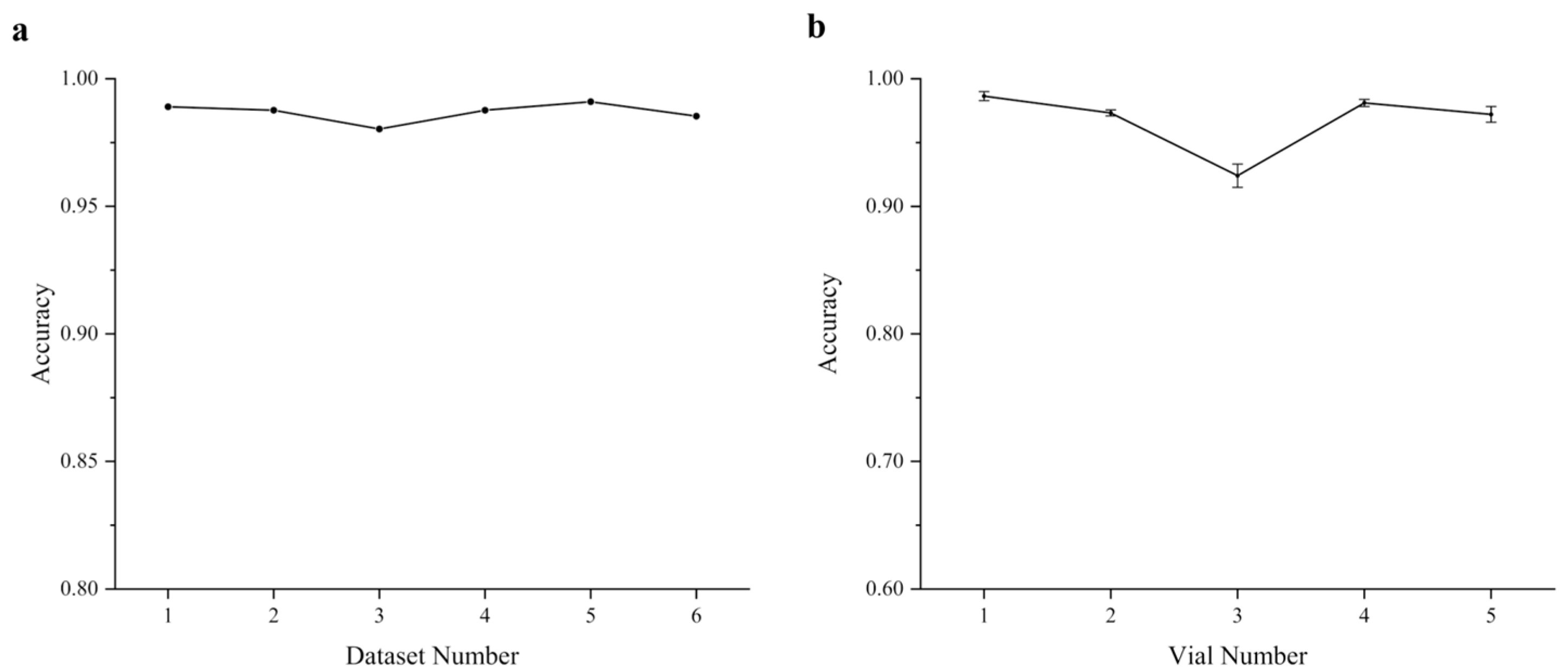
3.3. Inter-Vial and Intra-Vial Variability

We tested protein particles, which are the most stress-sensitive of the seven particles, to demonstrate the robustness of our classifier to both inter-vial and intra-vial variability in protein particles. Intra-vial variability was validated by using untrained images in the vial where the training set images were located. This was validated for a total of six groups, of which the first group was the test set of 2000 protein particles, and the other five groups each contained 3000 images. The results shown in Figure 5a indicate little variation in the accuracy of the new protein particles in the same vial—the accuracy was above 98% in all cases.

Figure 5b demonstrates the variability in the accuracy of protein particles within different vials using 3000 × 5 images from each of the different vials that entered the network. The results of the study show that the intra-vial variability was significantly higher than the inter-vial variability, as the accuracy fluctuations were more pronounced, as the fluctuations in accuracy were more pronounced. Nevertheless, the accuracy rates in different vials were over 92%, indicating that the protein particles were also robust for vial-to-vial differences. Overall, in our study, the CNN classifier is robust for both inter-vial and intra-vial variability of protein particles. This shows the network structure used is able to tolerate minor variations in the input image data, and has some generalization ability.

3.4. Machine Learning Classifiers for Particle Classification

We attempted to develop a machine learning method based on particle morphological features with single particles as the training set. In summary, 15 parameters were used as the training set for training the five machine learning algorithms, including an integrated classifier, a support vector machine, nearest neighbor classifier, discriminant analysis, and decision tree, which contained 24 classifiers in total. The total number of data points was 7 × 13,000 × 15. After 10-fold cross-validation, the five models with the highest accuracy rates were obtained and are shown in

Table 3. Top five classification performances of machine learning classifiers based on morphological features of images.

Accuracy Rank	Model	Train (Validation) Accuracy
1	SVM—Fine Gaussian SVM	87.70%
2	KNN—Weighted KNN	86.60%
3	SVM—Medium Gaussian SVM	86.30%
4	KNN—Three-time KNN	85.40%
5	KNN—Cosine KNN	84.40%

.

Compared with CNN, machine learning methods using single-particle morphological features show similar trends, as polystyrene beads are most easily identified and other particles are relatively less identifiable. However, even the complex machine learning method with the highest recognition rate, fine Gaussian support vector machine, had an overall recognition rate 9.79% lower than that of CNN, reaching 11.44% after excluding the standard particles and polystyrene spheres. This suggests that the CNN extracted more complex and more representative features when classifying these particles.

3.5. Pre-Trained and Scratch-Trained CNN

To compare transfer learning with network training from scratch, we used the training set described previously (9500 sheets × 7 classes) for the ImageNet transfer learning-based network and a network with random initialization parameters for each calculation. Each network was trained for 100 epochs, and the results show that the accuracies of both were almost equal, with 97.51% accuracy for the pre-trained VGG16 and 96.51% accuracy for the scratch-trained VGG16 when classifying seven particles. After 100 epochs of training, all networks showed convergence, with the pre-trained networks showing better performance in comparison, suggesting that the features learned from ImageNet can also assist in the classification of particles. In addition, transfer learning can be used with smaller sample sizes, and is more suitable for dataset collection under real conditions. Finally, transfer learning was effective in reducing the training time. In the scenario described herein, the pre-trained network only needs to train 8.92 million parameters in the fully connected layer, whereas the new training network needs to train 23.63 million parameters, which translates into a training time of 13.5 h for the scratch-trained network compared to 2.5 h for the pre-trained network.

Overall, the transfer learning property of CNNs can be generalized to the classification of subvisible particles. In our study, feature extraction was performed by using the convolutional base of VGG16 pre-trained on ImageNet, and then we used the labeled particle datasets to train the custom classifier and update the weights of the fully connected layer. Our results indicate that the transfer with fine-tuning of features learned from natural images is beneficial for subvisible particle representation, and provided better results than training from scratch. Based on the properties of transfer learning, the method is easier to generalize when compared to other studies. It has the potential to be used directly on the real dataset of industry production process without targeted major adjustments. Transfer with fine-tuning is expected to become a general method for the classification of subvisible particle types in pharmaceutical formulations.

4. Conclusions

This study applied VGG16 combined with high-resolution FlowCam images based on pre-trained ImageNet datasets for subvisible particle classification. Seven typical subvisible particles (extrinsic, intrinsic, and inherent) in standard solutions of water-based particles were manually prepared to simulate the particles observed during the production of injectable biotherapeutic pharmaceutical formulations. Based on the image information obtained from FlowCam, we built a dataset and trained our self-defined classifier on the convolutional base of VGG16 by pre-training the ImageNet dataset.

For the prepared images of standard particles above 5 µm, seven subvisible particles were predicted using the classifier described in this study. The test dataset achieved a prediction accuracy of 97.51% and more than 91% for each class of particles. In addition to accuracy, other evaluation metrics, such as recall, precision, ROC curve, and AUC, helped support the accuracy of the model. We also verified the robustness of the model against other particles in the same vial and particles in other vials under the same stress conditions using protein particles, and compared this with the machine learning method and the pre-trained VGG16. The results show that the pre-trained VGG16 was able to improve in accuracy by over 9.74% compared to the machine learning method. Pre-trained VGG16 requires less training time and is better adapted to the actual dataset collection compared to a CNN trained from scratch, and also demonstrates the possibility of applying the features learned from the ImageNet dataset to classify subvisible particles.

In summary, the application of transfer learning to FlowCam image analysis to identify subvisible particles provided a classification model with high prediction accuracy for images of standard particles. To improve the practical application of the model, further efforts should be made to extend the width of the model by preparing different particle samples with different materials, composites, or stress methods. By combining the ability of CNN for sub-category recognition, this study also has the potential to combine protein stress source classification [21] to achieve identification from particle type to stress source. Through these efforts, the optimized approach has the potential to facilitate the identification of subvisible particles in industrial processes, thereby increasing their practical value while improving accuracy. This may help in the tracing of particles, ultimately shortening the investigation of root causes and advancing process improvement and control.

References

1. Singh, S.K.; Afonina, N.; Awwad, M.; Bechtold-Peters, K.; Blue, J.T.; Chou, D.; Cromwell, M.; Krause, H.-J.; Mahler, H.-C.; Meyer, B.K.; et al. An industry perspective on the monitoring of subvisible particles as a quality attribute for protein therapeutics. J. Pharm. Sci. 2010, 99, 3302–3321. [Google Scholar] [CrossRef]
2. Visual Inspection of Injections. The United States Pharmacopeial Convention. 2017. Available online: https://www.pharmout.net/wp-content/uploads/2018/02/NGVF-2016-Visual-Inspections-of-Injection.pdf (accessed on 27 March 2022).
3. Wang, W.; Nema, S.; Teagarden, D. Protein aggregation—Pathways and influencing factors. Int. J. Pharm. 2010, 390, 89–99. [Google Scholar] [CrossRef]
4. Simler, B.R.; Hui, G.; Dahl, J.E.; Perez-Ramirez, B. Mechanistic complexity of subvisible particle formation: Links to protein aggregation are highly specific. J. Pharm. Sci. 2012, 101, 4140–4154. [Google Scholar] [CrossRef]
5. Kumru, O.; Liu, J.; Ji, J.A.; Cheng, W.; Wang, Y.J.; Wang, T.; Joshi, S.B.; Middaugh, C.R.; Volkin, D.B. Compatibility, physical stability, and characterization of an IgG4 monoclonal antibody after dilution into different intravenous administration bags. J. Pharm. Sci. 2012, 101, 3636–3650. [Google Scholar] [CrossRef]
6. Pardeshi, N.N.; Zhou, C.; Randolph, T.W.; Carpenter, J.F. Protein nanoparticles promote microparticle formation in intravenous immunoglobulin solutions during freeze-thawing and agitation stresses. J. Pharm. Sci. 2018, 107, 852–857. [Google Scholar] [CrossRef]
7. Joubert, M.K.; Hokom, M.; Eakin, C.; Zhou, L.; Deshpande, M.; Baker, M.P.; Goletz, T.J.; Kerwin, B.A.; Chirmule, N.; Narhi, L.O.; et al. Highly Aggregated Antibody Therapeutics can enhance the in vitro innate and late-stage T-cell immune responses. J. Biol. Chem. 2012, 287, 25266–25279. [Google Scholar] [CrossRef] [Green Version]
8. Chisholm, C.F.; Soucie, K.R.; Song, J.S.; Strauch, P.; Torres, R.M.; Carpenter, J.F.; Ragheb, J.A.; Randolph, T.W. Immunogenicity of structurally perturbed hen egg lysozyme adsorbed to silicone oil microdroplets in wild-type and transgenic mouse models. J. Pharm. Sci. 2017, 106, 1519–1527. [Google Scholar] [CrossRef]
9. Fathallah, A.M.; Chiang, M.; Mishra, A.; Kumar, S.; Xue, L.; Middaugh, C.R.; Balu-Iyer, S.V. The effect of small oligomeric protein aggregates on the immunogenicity of intravenous and subcutaneous administered antibodies. J. Pharm. Sci. 2015, 104, 3691–3702. [Google Scholar] [CrossRef]
10. Kotarek, J.; Stuart, C.; De Paoli, S.H.; Simak, J.; Lin, T.-L.; Gao, Y.; Ovanesov, M.; Liang, Y.; Scott, D.; Brown, J.; et al. Subvisible particle content, formulation, and dose of an erythropoietin peptide mimetic product are associated with severe adverse postmarketing events. J. Pharm. Sci. 2016, 105, 1023–1027. [Google Scholar] [CrossRef] [Green Version]
11. Particulate Matter in Injections, the United States Pharmacopeial Convention. 2006. Available online: https://www.uspnf.com/sites/default/files/usp_pdf/EN/USPNF/revisionGeneralChapter788.pdf (accessed on 27 March 2022).
12. Zölls, S.; Weinbuch, D.; Wiggenhorn, M.; Winter, G.; Friess, W.; Jiskoot, W.; Hawe, A. Flow imaging microscopy for protein particle analysis—A comparative evaluation of four Different Analytical Instruments. AAPS J. 2013, 15, 1200–1211. [Google Scholar] [CrossRef] [Green Version]
13. Demeule, B.; Messick, S.; Shire, S.J.; Liu, J. Characterization of particles in Protein Solutions: Reaching the limits of current technologies. AAPS J. 2010, 12, 708–715. [Google Scholar] [CrossRef] [Green Version]
14. Methods for Detection of Particulate Matter in Injections and Ophthalmic Solutions. The United States Pharmacopeial Convention. 2018. Available online: https://www.usp.org/ (accessed on 27 March 2022).
15. Narhi, L.O.; Corvari, V.; Ripple, D.C.; Afonina, N.; Cecchini, I.; Defelippis, M.R.; Garidel, P.; Herre, A.; Koulov, A.V.; Lubiniecki, T.; et al. Subvisible (2–100 Μm) particle analysis during biotherapeutic drug product development: Part 1, Considerations and Strategy. J. Pharm. Sci. 2015, 104, 1899–1908. [Google Scholar] [CrossRef]
16. Strehl, R.; Rombach-Riegraf, V.; Diez, M.; Egodage, K.; Bluemel, M.; Jeschke, M.; Koulov, A.V. Discrimination between silicone oil droplets and protein aggregates in biopharmaceuticals: A novel multiparametric image filter for sub-visible particles in microflow imaging analysis. Pharm. Res. 2012, 29, 594–602. [Google Scholar] [CrossRef]
17. Lecun, Y.; Bengio, Y.; Deep Learning, H.G. Deep learning. Nature 2015, 521, 436–444. [Google Scholar] [CrossRef]
18. Rawat, W.; Wang, Z. Deep convolutional neural networks for image classification: A comprehensive review. Neural Comput. 2017, 29, 2352–2449. [Google Scholar] [CrossRef]
19. Esteva, A.; Kuprel, B.; Novoa, R.A.; Ko, J.; Swetter, S.M.; Blau, H.M.; Thrun, S. Dermatologist-level classification of skin cancer with deep neural networks. Nature 2017, 542, 115–118. [Google Scholar] [CrossRef]
20. Kerr, T.; Clark, J.R.; Fileman, E.S.; Widdicombe, C.E.; Pugeault, N. Collaborative deep learning models to handle class imbalance in flowcam plankton imagery. IEEE Access 2020, 8, 170013–170032. [Google Scholar] [CrossRef]
21. Calderon, C.P.; Daniels, A.L.; Randolph, T.W. Deep convolutional neural network analysis of flow imaging microscopy data to classify subvisible particles in protein formulations. J. Pharm. Sci. 2018, 107, 999–1008. [Google Scholar] [CrossRef] [Green Version]
22. Daniels, A.L.; Calderon, C.P.; Randolph, T.W. Machine learning and statistical analyses for extracting and characterizing “fingerprints” of antibody aggregation at container interfaces from flow microscopy images. Biotechnol. Bioeng. 2020, 117, 3322–3335. [Google Scholar] [CrossRef]
23. Gambe-Gilbuena, A.; Shibano, Y.; Krayukhina, E.; Torisu, T.; Uchiyama, S. Automatic identification of the stress sources of protein aggregates using flow imaging microscopy images. J. Pharm. Sci. 2020, 109, 614–623. [Google Scholar] [CrossRef] [Green Version]
24. Umar, M.; Krause, N.; Hawe, A.; Simmel, F.; Menzen, T. Towards quantification and differentiation of protein aggregates and silicone oil droplets in the low micrometer and submicrometer size range by using oil-immersion flow imaging microscopy and convolutional neural networks. Eur. J. Pharm. Biopharm. 2021, 169, 97–102. [Google Scholar] [CrossRef]
25. Huh, M.; Agrawal, P.; Efros, A.A. What makes ImageNet good for transfer learning? arXiv 2016, arXiv:1608.08614. [Google Scholar]
26. Simonyan, K.; Zisserman, A. Very deep convolutional networks for large-scale image recognition. arXiv 2015, arXiv:1409.1556. Available online: https://arxiv.org/abs/1409.1556 (accessed on 27 March 2022).
Figure 1. Illustration of the transfer learning workflow. The VGG16 network was trained on the ImageNet dataset, and the convolutional base of the trained network plus the custom three-layer classifier formed the network used in this study. The fully connected layer of this network was trained using particle images obtained from FlowCam (the transferred convolutional base was frozen) to achieve the classification of seven classes of particles. CNN: convolutional neural network.
Applsci 12 05843 g001
Figure 2. Sample FIM images from seven classes of particles: (a) glass particles, (b) cap fiber particles, (c) rubber closure particles, (d) protein particles, (e) silicone oil microdroplets, (f) silicone tubing particles, and (g) polystyrene beads. FIM: flow imaging microscopy.
Applsci 12 05843 g002
Figure 3. Confusion matrix of our CNN, tested on 2000 images from each class with an overall classification efficiency of 97.51%.
Applsci 12 05843 g003
Figure 4. ROC curve and area under the curve of the model and each class. The ROC curve is the graphical display of sensitivity (TPR) on the y-axis and 1-specificity (FPR) on the x-axis for varying cut-off points of test values. An area under the curve closer to 1 indicates better performance of the test. ROC: receiver operating characteristic.
Applsci 12 05843 g004
Figure 5. Intra-vial and inter-vial variability of protein particles. (a) Accuracy of test protein image data within the same vial as the training set. Dataset number 1 means the test set containing 2000 test images; numbers 2–6 each contained 3000 test images in the same bottle. (b) Accuracy of test protein image data between different vials. Each vial number means an individual vial containing 5 × 3000 protein images; Vial 1 was where the training data were located. The accuracy was averaged over five sets of images. The test images above were not used in training.
Applsci 12 05843 g005