Analysis of Recent Mean Temperature Trends and Relationships with Teleconnection Patterns in California (U.S.)

Abstract

The global mean surface temperature has risen since the late 19th century. However, temperatures do not increase uniformly in space or time and few studies have focused on that peculiarity in the State of California. The aim of this research is to deepen our knowledge of the evolution of mean temperatures in the State of California on monthly, seasonal and annual time scales. The period under study comprises 40 years (from 1980 to 2019) and data from 170 meteorological stations were analysed. Statistical techniques, including Sen’s slope and Mann-Kendall, were applied to each of the stations to establish the sign and slopes of trends and their statistical significance. The spatial distribution of monthly, seasonal and annual trends was analysed using the Empirical Bayesian Kriging (EBK) geostatistical technique. The trend analysis was also carried out for the State as a whole. This research also studies the relationships between mean temperatures and nine teleconnection patterns with influence on the Californian climate. To find out these links, a correlation analysis was performed using the partial non-parametric Spearman Test at a 95% confidence level. The study reveals a positive trend of +0.01 °C year⁻¹ for the whole state and that Southern California is getting warmer than Northern California for the study period. On a seasonal scale, the local temperature increased significantly both in autumn and summer (+0.06 °C and +0.035 °C year⁻¹ respectively) from 1980 to 2019. On a monthly scale, the largest increases are found in November at +0.04 °C year⁻¹. Temperatures in February, March, April and May are highly correlated with most of the teleconnection patterns studied in the State of California. West Pacific Oscillation (WPO) teleconnection pattern has shown the highest negative correlation. However, The Pacific Decadal Oscillation (PDO) has a positive correlation with mean temperatures in coastal areas such as Los Angeles, San Francisco and Monterey. Moreover, Antarctic Oscillation (AAO) and Arctic Oscillation patterns (AO) are unlikely to show great influence on average temperature trends in California.

1. Introduction

Global warming is one of the current challenges that human beings have to face due to its negative effects on society, such as floods [1], heat waves, wildfires and droughts [2], which are becoming more and more serious over time. The impacts on ecosystems and human well-being and health are associated with an increase in average temperatures [3,4]. The most significant evidence of this Global warming is the increase in air temperature [5]. The global mean surface temperature has risen since the late 19th century [6]. Each of the last four decades has been successively warmer than any decade that preceded it since 1850. The first two decades of the 21st century (2001–2020) were 0.99 [0.84–1.10] °C higher than 1850–1990. The global surface temperature was 1.09 [0.95–1.20] °C higher in 2011–2020 than 1850–1900, with larger increases over land (1.59 [1.34–1.83] °C) [7]. It is practically certain that the minimum and maximum temperatures of the Earth’s surface have increased on a global scale since 1950 [8]. In addition, recent studies suggest that there are slight differences between the changes in the maximum and minimum temperatures and these can be easily altered by human activity and land uses at a regional level [9].

Climate is variable in time and space, so detecting a significant trend is a great challenge for researchers. The calculation of trends in climatic elements such as average temperature, maximum and minimum temperature has been the subject of a great number of studies in recent years [6,10,11,12,13,14,15,16] and has been carried out in a wide variety of territories around the world. Most of the studies at this point have focused on large-scale temperature trends. However, it is necessary to carry out more research to focus on the change that occurs at a regional level using the above-mentioned parameters. In this way, research carried out on decadal trends in average temperatures in various territories of the United States provides impressive results. Average temperatures across the US have increased from the 1950s to the beginning of the century by more than 0.5 °C [6,10,12,13,14,17].

In order to study how global warming would affect life at a regional level, models and assessments of climate change often assume that the influence would be uniform. However, temperatures do not increase uniformly in space or time and few studies have focused on that peculiarity in California State [18,19,20]. In general, the colder hours of the day (nights), the coldest times of the year (winter), and the colder parts of the world (high latitudes) tend to heat up faster. Although, and in contrast to this, in the State of California, temperatures have undergone great variations over the last 100 years, with greater warming being experienced in the southern desert territories [18,21]—where temperatures were regularly high—while in the northern territories, increases have taken place gradually. To be more precise, these temperature increases are uneven for the different regions of the centre and north of the State.

Several climatological research papers have suggested that much of the current climate variability observed can be related to variability within a teleconnection pattern [22,23,24]. The term teleconnection pattern refers to a large-scale recurring pattern that persists over time with pressure and circulation anomalies that extend to wide geographic areas. In addition, sometimes these patterns can last for several consecutive years. There are some patterns of teleconnection that can directly or indirectly influence the monthly temperatures of a region of the planet such, as the United States [22,25,26,27,28,29], or act on a smaller spatial scale, such as the State of California [30,31,32,33,34]. Teleconnection patterns that may influence the United States, including tropical patterns that could affect the southern territories, are Antarctic Oscillation (AAO), Arctic Oscillation (AO), North Atlantic Oscillation (NAO), Pacific–North American Pattern (PNA), Madden Julian Oscillation (MJO), West Pacific Oscillation (WPO), described by both Barnston and Livezey [35] and Wallace and Gutzler [36], and the Eastern Pacific (EPO), whereas in the State of California, they are mainly El Niño along the Southern Oscillation (ENSO) [24,37,38] and the Pacific Decadal Oscillation (PDO) [19,39,40]. Although effects of teleconnection patterns on California climate variables such as precipitation have been studied before, temperature change and its relationship to teleconnection patterns need further investigation.

Previous studies have revealed that the climate in California is changing, but how important and what has been the quantitative change in California? Does it occur in a homogeneous way throughout the territory? These are still unsettled questions. With this research, it is our intention to help respond to these enquiries. There is a lack of current data on recent temperature trends that consider those extreme temperature events that have occurred in California from 2013 to the present. To our knowledge, there has never before been an investigation analysing monthly, seasonal and annual values of mean temperature trends for the State of California in such a current period (1980–2019) in contrast to previous studies [18,19]. Therefore, one of the objectives and originality of this research lies in expanding the knowledge of the spatial and temporal evolution of mean temperature trends for the entire State of California as a whole and each of the weather stations studied.

As we have seen, previous research has focused on the correlations of some atmospheric teleconnection patterns with temperatures over short periods of time, for example, during a year or in isolated seasonal periods such as in winter. In addition, there is more knowledge available on possible links between teleconnection patterns with precipitation [9,41,42,43,44,45] than with temperatures. Consequently, the other objective of this work is to analyse the possible relationship between mean temperatures and up to nine different teleconnection patterns that are most influential in the Californian climate.

Finally, the authors believe that the findings of this study will help land managers to take appropriate measures in advance of global warming, thus helping them to minimise the effects of this phenomenon.

2. Materials and Methods

2.1. Study Area

This study is carried out in the State of California, the third-largest state in the United States, with an area of 423.955 km². Its orography varies from 84.1 m below sea level in Death Valley to 4418.1 m above sea level on the peak of Mount Whitney [46]. California includes two major series of mountain ranges: The Coastal Range and the Sierra Nevada, plus the southern tip of the Cascade Range, including Mount Lassen and Mount Shasta. Between these two axes lies the Greater Central Valley, whose Sacramento and San Joaquin river systems drain through Golden Gate (Figure 1). California’s climate is highly variable, and the area ranges from desert to subalpine environments [47]. Its complex topography and great latitudinal extension favour a wide variety of climates. Thus, its proximity to the Pacific coast is one of the determining factors in the climate of the state. A Mediterranean climate predominates throughout the state, except for the mountain area of Klamath, where there is a temperate climate and the southeast in the Sonoran Desert, where we find a tropical climate [48].

2.2. Data

A total of forty years (from 1980 to 2019) was selected as the study period. Three decades are recommended by the World Meteorological Organization (WMO) to carry out climatic studies. We initially worked with a database of 350 meteorological stations containing monthly average temperature data available on the Western Regional Climate Center (WRCC) website [49]. The meteorological stations were selected considering criteria of completeness, length and homogeneity to cover most of the state [50]. Only stations with less than 10% of missing values were chosen. Those missing gaps were completed with the corresponding monthly long-term mean value [51].

Homogeneity analysis of the series was also carried out. In this study, it was determined by the Run test [52], with a confidence level of 99%. This test is recommended by the World Meteorological Organization (WMO) because it does not require the analysed series to come from a normal sample and it has also been previously used by other climatic studies [53,54]. After the elimination of the meteorological stations with missing data and homogeneity analysis, we finally worked with 170 stations (Figure 1). The altitude values and geographic coordinates of each of the stations used were also added to the database to ease the representation of the results obtained on maps at a later date.

Monthly values were averaged for each meteorological station to obtain seasonal and annual series. In California, 4 seasons are considered: Winter (December, January and February), spring (March, April and May), summer (June, July and August) and autumn (September, October and November). From now on, the seasons will be named DJF, MAM, JJA and SON, respectively.

For the whole State of California, the monthly, seasonal and annual temperature was computed using Voronoi polygons weighting temperature stations by the area of each polygon [55].

2.3. Trend Analysis

The trend analysis was carried out using the Mann-Kendall test together with the Sen slope estimator. The non-parametric Mann-Kendall test, referred to as the Kendall tau test, is one of the most widely accepted non-parametric tests for detecting trends in time series [50,54,56,57]. The Mann–Kendall test was applied, as in other research [58], as follows:

$$S={{\displaystyle \sum }}_{i=1}^{n-1}{{\displaystyle \sum }}_{j=i+1}^{n}sgn\left(x_j-x_i\right)$$

$$sgn\left(x_j-x_i\right)=\{\begin{array}{c}1 \mathrm{if} x_j-x_i>0\\ 0 \mathrm{if} x_j-x_i=0\\ -1 \mathrm{if} x_j-x_i<0\end{array}$$

where n is the length of the sample, $x_j$ and $x_i$ are from i = 1, 2, …, n − 1 and j = i + 1, …, n. 34. For n > 8, S is approximately normally distributed. The mean of S is 0 and the variance of S can be obtained as follows:

$$V\left(S\right)=\frac{n\left(n-1\right)\left(2n+5\right)-{{\displaystyle \sum }}_{1=1}^n{t}_{i}i\left(i-1\right)\left(2i+5\right)}{18}$$

The standardized test statistics (z) of the MK test and the corresponding p-value (p) for the one-tailed test are respectively given as follows:

$$Z=\{\begin{array}{c}\frac{S-1}{\sqrt{Var\left(S\right)}} S>0\\ 0 S=0\\ \frac{S+1}{\sqrt{Var\left(S\right)}} S<0\end{array}$$

If Z > 0, it indicates an increasing trend and vice versa. Given a confidence level α, the sequential data would be supposed to experience a statistically significant trend if |Z| > Z(1 − α/2), where Z(1 − α/2) is the corresponding value of P = α/2 following the standard normal distribution. In this study, a 0.05 confidence level was used.

The slope of the linear trend is estimated with the nonparametric Sen slope estimator. It is a non-parametric procedure that estimates changes per unit of time in a series when there is a linear trend [59,60,61]. It allows to estimate the slope fitting a set of (time, $x$ variable) elements in a non-parametric way, being much less sensitive to outliers. It is the median of all the slopes calculated between all the time instants whenever instant i is less than instant j.

Sen’s slope is defined as

$$Sen’sslope=median\left\{\left(\frac{x_j-x_i}{j-i}\right)\forall i<j\right\}$$

The Modified Sen’s slope aims to remove the autocorrelation of the $x$ variable before computing the slopes. The trend of $x$ time series is computed using an autoregressive model of order 1, an AR (1) model.

With the autoregressive term $\rho$ a new series $x^{\prime }$ (with n − 1 elements) is constructed:

$$x^{\prime }=x\left\{i=2,3,\dots ,n\right\}-x\left\{i=1,2,3,\dots ,n-1\right\}\rho$$

Sen’s slope formula is applied considering the $x^{\prime }$ transformed series and time values from 1 to n − 1.

The modified Sen slope [62] was applied in this research. R package version 4.1.0 was used both to carry out the slope calculations, obtained with a modified Sen’s slope method and the Mann-Kendall test [63]. All trend analysis was carried out at monthly, seasonal and annual temperature levels.

Statistical interpolation of the values is necessary for a specific region. In order to carry out this interpolation, ArcGis 10.8 © [64] software was used and, more specifically, an Empirical Bayesian Kriging geoprocessing tool (EBK). It is a method of interpolation of geographic statistics where the standard errors of the prediction are more precise than in other kriging methods [65,66,67]. In addition, 17 average temperature trend contour maps were designed with ArcGis 10.8 © and statistically significant areas, at a 95% confidence level, were also superimposed onto the contour maps.

2.4. Atmospheric Teleconnection Patterns

Values of atmospheric circulation pattern indices were taken both from the Climate Prediction Center available on the NOAA National Climatic Data Center (NCDC) website (https://www.ncdc.noaa.gov/teleconnections/ accessed 4 May 2020), similar to previous research [18,27,39]. Due to the lack of Real-Time Multivariate Madden-Julian Oscillation (RMM) indices in NCDC, these indices were obtained from the Australian Bureau of Meteorology (http://www.bom.gov.au/climate/mjo/graphics/rmm.74toRealtime.txt accessed 1 June 2020). We have chosen each one of the teleconnection patterns that can influence climate in the United States and the State of California. Namely El Niño 3.4 (ENSO) and the Pacific Decadal Oscillation (PDO) [31,68], besides the Antarctic Oscillation (AAO), Arctic Oscillation (AO), Madden-Julian Oscillation (MJO), North Atlantic Oscillation (NAO), Pacific–North American Pattern (PNA), West Pacific Oscillation (WPO) and East Pacific Oscillation (EPO) were also taken in consideration.

To find out the relationships between temperature and teleconnection patterns in California a correlation analysis using the partial non-parametric Spearman Test was performed at a 95% confidence level [63]. This method (the Spearman test) assigns less significance to outliers and is a more robust and resistant alternative for measuring correlation (linear or nonlinear). In addition, this partial test eliminates the effect that the time variable can exert on the temperature and telepattern variables to avoid fictitious relationships [51]. Finally, all the correlation results and their statistical significance are represented in monthly maps.

3. Results and Discussion

3.1. Temperature Trends

In this section, two different approaches to studying temperature trends are considered.

Firstly, the results of the trend analysis of temperature for the entirety of California (

Table 1. Mean temperature trends (°C year⁻¹) for the entire State of California. * Statistical significance at a 95% confidence level.

	January	February	March	April	May	June	July	August	September
Slope	0.04	0	0.02	0.02	0.01	0.03	0.03	0.03	0.01
p value	0.06	0.87	0.37	0.53	0.44	0.07	0.03 *	0.01 *	0.23
	October	November	December	Winter	Spring	Summer	Autumn	Annual
Slope	0.01	0.04	0.02	0.02	0.01	0.03	0.03	0.01
p value	0.58	0.02 *	0.25	0.25	0.38	0.02 *	0.02 *	0.13

) show that a positive trend exists in the state as a whole. The highest value is found in November (+0.04 °C year⁻¹) and it is statistically significant. The same arises with July, August, summer and autumn, where the trend reaches +0.03 °C per year. It is noteworthy that January has shown the same trend (+0.04 °C year⁻¹) over the period studied as November but is not statistically significant. It is remarkable that February has shown no trend.

Secondly, the results of analysing temperature trends (positive and negative) for each one of the meteorological stations on monthly, seasonal and annual levels from 1980 to 2019 in the State of California as well as their statistical significance at a confidence level of 95% are shown in Figure 2 and Figure 3.

Figure 2 shows that at least 60% of the meteorological stations showed positive trends for each month, in the different seasons and on an annual scale with the highest fraction of positive trend in November, reaching 92% of the stations. Alternatively, it was revealed that January, June, July, August and November are the months that have shown the highest percentages of stations with statistical significance. In November, significant trends are observed in almost half of the stations studied (40%). In addition, autumn is the season that showed the highest percentage of meteorological stations with positive trends (90%) and 35% of them statistically significant. In spring, however, only 72% of the trends are positive and only are 4% statistically significant. In contrast to other months, 57% of the trends in February are negative but none of them are statistically significant.

According to the monthly results (Figure 3), in January the spatial distribution of positive trends was found all over the state, close to 80% of the stations as can be seen in Figure 2. The highest increases (+0.056 °C year⁻¹) were found in the Sacramento and San Joaquin Valley, where 30% of the stations were statistically significant. Although the observational period and time scale are different (1910–2003), our result agrees with the research [69] that revealed a rise in annual mean temperatures in this area. This rapid warming in the Valley seems to be caused by the development of irrigated agriculture [70] in contrast to the slight increase they had shown in Sierra Nevada. Irrigated agriculture increases the minimum temperature (T_min) values in these areas and seems not to have an effect on maximum temperatures (T_max), which explains the increase in mean temperatures. The San Joaquin and Sacramento rivers that originate in the Sierra Nevada and the mountainous regions in the north run through this region. The confluence of the rivers occurs in the Sacramento–San Joaquin Delta. Most of the water from these rivers comes from snowmelt, and the increase in temperature trends in the winter season (DJF) would mean acceleration in the snow melting season. These results agree with other research conducted in other mountain systems [71]. In those three months, high positive trends (+0.02–0.03 °C year⁻¹) have been found all over California, in nearly 90% of the stations (Figure 2). That rapid melt can cause difficulties in the maintenance of fresh water in agriculture and for human consumption, as suggested by some researchers [47,72,73,74]. The Central Valley can be more vulnerable to warming-driven drought if reductions in water supply cause reductions in irrigation [75].

The map for February (Figure 3) revealed a lack of clear trends due to the fact that there is no distinct direction in positive or negative temperature trends. These findings support the results shown on the NOAA website (https://www.ncdc.noaa.gov/temp-and-precip/us-trends/ accessed 10 February 2021), which points out that “strong trends are not shown, this is because the period studied is defined by warm Februarys in the 90’s and cold ones in 00’s in California State”.

We can see (Figure 3) great similarities in both March and April temperature trends. During these months, the northeast of California tends to show slightly negative temperature trends in 30% of the stations (−0.01 °C year⁻¹), while in South Sierra Nevada, the Mojave Desert, Los Angeles, Imperial Valley, San Gabriel and San Bernardino Mountain, the average temperature had gone up +0.04 °C year⁻¹. The results in May for California are different from the rest of the year because, in the southern coastal region and San Francisco Bay, a negative trend appeared (−0.01 °C year⁻¹). This could be related to the penetration of coastal marine fog, which varies seasonally [76]. That is important due to the moisture content of air near the surface, making this a regional phenomenon with strong local patterns [77]. This cooling effect that we have mentioned before has been explained by previous investigation [78], although in this research it seems to have a lesser effect—instead of being negative, trends are close to zero, similar to what has been mentioned in other research. In fact, coastal fog along the California coast, critical to San Francisco Bay Area climate, is less frequent than before [79].

During June, July and August, the temperature has risen all over the State (+0.065 °C year⁻¹), showing more territories with statistically significant trends in July and August (30% of the stations analysed). Figure 3 shows highly significant trends in these months in the northern part of the State, Mt. Shasta, part of the Cascade Ranges and Lake Tahoe, and a huge area of Death Valley and the Mojave Desert. These results are related to those which confirm increases in trends of heat waves in south California [80], becoming more and more frequent in urban environments than in more rural surroundings. As a result of this is a higher risk of heat-related births [81] and deaths as well as an increase in wildfires. Increases of +0.05 °C year⁻¹ in Sacramento and San Joaquin Valley are in this research comparable to June and August.

The trends in September show great similarities to July and August but with less statistically significant areas. Nevertheless, in October, there was a negative trend (−0.01 °C year⁻¹) without statistical significance in the north, particularly in coastal areas, covering Eureka city up to Shelter Cove, as had been stated by previous research [18]. In the case of November, the western coastal zone is cloudy and mild, and northern areas are rather cooler than the southern, reaching an average temperature of 17 °C in some years. The results for this month showed both positive trends (+0.05 °C year⁻¹) and statistical significance in Sacramento and San Joaquin Valley, Sierra Nevada, Los Angeles, San Francisco Bay, Yosemite and Southern Lake Tahoe.

Last but not least, December showed a positive trend in most of California, with the exception of the northwest, where it has been noted a negative trend with a decrease of 0.02 °C year⁻¹ during the period studied, although it is not statistically significant. In addition, the territories of Sacramento and San Joaquin Valley showed the highest increases with statistical significance (+0.032 °C year⁻¹). As we have previously pointed out, this is a rising concern due to the fact that snowmelt increases in mountain areas probably causing a shortage in water supply in the months to come.

Focusing on the seasonal trends (Figure 3), it is especially striking that both summer and autumn have shown statistically significant positive trends (+0.03 °C year⁻¹). The area with statistical significance spreads over the Mojave Desert and Death Valley, supporting the idea mentioned before that the south of California is warming more than the north of the State. In summer, the warming trend increases towards the interior of the State as we move away from the coast, where the trend is very small and statistically insignificant. These results agree with previous studies that have reported a cooling trend. These drop-in average temperatures could be due to a wide range of factors, such as irrigation, coastal upwelling or cloud cover [56,78]. The increase in temperatures over inland areas increases sea-breeze flow activity [19,78] lowering the temperatures in coastal zones of the State.

The spatial distribution of winter trends allows us to discriminate between two distinct areas: one formed by the territories of the Klamath Mountains and the other by the north of the Cascade Range, where we find a statistically insignificant negative trend. The rest of the territory in this season has shown a positive trend of +0.02 °C year⁻¹. It is noteworthy that this value is statistically significant in Sacramento and San Joaquin Valley and the south of Sierra Nevada. The trend in spring has shown clear warming throughout the territory but with slight statistical significance.

Finally, the spatial distribution of annual trends represented in Figure 3 reflected clear warming in the territory, +0.015 °C year⁻¹, except for the northern area, in the Klamath Mountains, where there is no clear trend. This issue has been addressed previously by He and Gautam (2016). It can also be observed that this positive trend in the territory is especially large in the south of the State, with statistical significance in the southeast of Sierra Nevada, coinciding with the Valley of Death and much of the Mojave Desert. These results accord with those proposed by Cordero et al. (2011) during 1918–2006 for the maximum and minimum temperature trends since both parameters show a significant rising in the southern part of the State.

The whole State getting warmer has concerning implications, such as the snow on the mountainous systems of California melting earlier in winter–spring, which is likely to decrease the water supply even further next season [73,82]. In addition, more heat produces more evaporation and so irrigation farmland would need more water, increasing the lack of fresh water even more. All in all, over the period of study, as can be seen in Figure 2 and Figure 3, no negative statistically significant trends were found in California.

Several investigations suggest that these differences in the increase in temperature are affected by several factors; some of them are anthropic activity, land use and the emission of greenhouse gases [9,83]. Greenhouse gases appear to be related to the increase in average temperatures and the impact derived from this increase [73]. Research on the possible causes of the increase in temperature in the State of California shows that the existing changes in atmospheric teleconnection patterns have significantly altered the extreme temperature events that take place in the said region [20]. There is a concrete example in the North Pacific Ocean, where surface temperatures correlate highly with Californian temperatures [84]. Finally, a great deal of climatological research suggests that temperature variability can be related to variability within the atmospheric flow [22].

3.2. Teleconnection Patterns

This section shows the results of the spatial and statistical analysis between temperatures and nine teleconnection patterns. Figure 4 shows the percentage of meteorological stations with a statistically significant positive (+) or negative (−) correlation between the teleconnection patterns and the mean temperature in California. The results of the correlations of atmospheric teleconnection patterns and temperatures are presented in a heat map outlining the highest values in dark red and the lowest in light red, following previous investigations [53,57,85,86,87].

The general circulation of the atmosphere displays significant variability on many diverse time scales. The chosen modes of low-frequency atmospheric variability have been labelled as teleconnections [22]. They are the main cause of weather anomalies that occur for a long period over different regions. In addition, these teleconnections patterns have an effect on temperature and precipitation regimes [88]. Particularly, in our research, temperatures in February, March, April and May are highly correlated with most of the teleconnection patterns in the State of California.

The Pacific Decadal Oscillation (PDO) is a teleconnection pattern of North Pacific sea surface temperature that alternates phases every 20–30 years [88]. A remarkable characteristic is that this index shows multiyear and multidecadal persistence with just a few signs of change [68]. Figure 5 shows that this pattern has a constant positive correlation with mean temperature. This pattern reveals that it might have more influence on the average temperature in California’s coastal areas such as San Francisco, Monterey Bay, Los Angeles and San Diego. We can observe in the maps that the highest percentage of stations with positive correlation is found along the coast as previous studies have brought to the fore [18,19]. This is most notable in May, when 19.2% of stations were statistically significant, followed by June (30%), September (33%) and October (38%). In March, when the percentage of stations with a significant correlation is the largest, there was no difference between coastal and interior locations in the State. The remarkable predominance of significantly positive correlations (Figure 4) allows us to say about PDO is probably that it is related to increases in average temperatures all over California in the period studied.

The correlations between PNA pattern and temperature have been strongly positive in February (Figure 6). In this month, 82% of the stations all over California have shown a positive and statistically significant correlation. During the months of June and August, this pattern has shown a negative correlation throughout the territory studied (30.2% and 28.5% respectively of meteorological stations), mainly in southern areas of the State. It is remarkable that at the end of autumn and the whole winter, a positive correlation is found mainly in North California’s meteorological stations. This is consistent with other research carried out in the United States, where the authors showed that there is a high correlation in the increase of temperature in winter due to this pattern [27,41]. Positive phases of Pacific–North America (PNA) are associated with above-average temperatures in the western and below-average temperatures in south-eastern U.S. The PNA pattern has its largest variability during winter [89].

Amongst the teleconnection indices studied, the Western Pacific Oscillation (WPO) has the highest percentage of statistically significant negative correlations with temperature (Figure 7). From December to April, high correlation values between WPO and temperatures were observed throughout the territory with 42.4% (January) to 95.9% (March) of the stations having significant negative correlations. However, no precise spatial area of influence can be identified for this pattern. We have to take into account that WPO is a temporary pattern and this could explain why it mainly affects the temperatures of winter [30] and spring months in the State of California (Figure 4 and Figure 7).

Furthermore, PDO and PNA are the two teleconnection patterns that display a high percentage of stations with significant positive correlation while WPO has shown the highest percentages of negative correlation. These results bear striking similarities with previous investigations undertaken in California with different surveillance periods [19,22,90].

If we consider the results regarding the Eastern–Pacific Oscillation (EPO) (Figure 8), we can state that 57.0% of stations have shown a significant positive correlation in November along with PNA and, to a lesser extent, PDO. Positive phases of EPO happen when pressure values are maintained in Alaska and high pressure is found in the northeast of Hawaii. This affects east California, making winters warmer than normal. In December, the EPO pattern had no data because there were no values available for the period studied on the datasheet of the Climate Prediction Centre (CPC, NOAA). Searching for alternative values for this pattern in December was not considered in order not to mix diverse information sources. This pattern shows especially high values of positive correlation in April, where 77.9% of the temperature in the stations studied seems to be affected by EPO.

Moving on to the North Atlantic Oscillation (NAO) (Figure 9), the highest percentage of stations (88.4%), with positive correlations between NAO and the temperature found in April and this percentage also high in May (56.4%) and March (40.7%). In this regard, strong positive phases of NAO are associated with above-average temperatures in the southern United States including California. This is supported by another recent investigation, where a substantial link between NAO and surface air temperatures over California during the March–June period was found [91]. Lastly, we can point out that NAO might influence temperatures for five months, from March to July, throughout California.

In contrast to NAO, significant correlations between ENSO 3.4 and temperature in California are infrequent and mainly linked at some coastal stations in February and March (Figure 10). These results concur with earlier research that highlights the slight correlation with temperature [18].

The Madden–Julian Oscillation (MJO) is both a global-scale complex teleconnection pattern of the tropical atmosphere and the dominant mode of intraseasonal tropical variability [85]. One commonly used index for defining MJO is the real-time multivariate index RMM. The two principal components RMM1 and RMM2 have been shown to be useful indices of the MJO and related variability [90]. Firstly, MJO is represented as a two-dimensional phase space defined by RMM1 and RMM2. The union of these two gives as a result eight equatorial phases of this teleconnection pattern. In the light of the results of the correlation of these indexes with the average temperature in California, January and November are the months that showed the highest positive correlation. More precisely, RMM1 (Figure 11) did not seem to have any relation with temperatures over the period studied in California while RMM2 (Figure 12) showed the highest percentage of significant positive correlation in November (41.3%) and January (20.3%). One of the reasons for these results, which are consistent with other research, could be that RMM1 describes the situation when an MJO produces enhanced convection at the Maritime Continent while RMM2 has enhanced convection over the Pacific Ocean [86,87] closer to California State. Dasgupta et al. (2020) found that the occurrences of MJO activity at RMM phase locations 4, 5 and 6 during boreal winter are related to the PDO index, particularly in the negative phases. Phases 6–7 of MJO are related to the convective anomaly in the western Pacific that affects the weather in the United States, where warm anomalies were found particularly in mid-latitude temperature and probably related to PNA [85].

The Arctic (AO) and Antarctic Oscillation (AAO) showed in most months less correlation with temperature than the other teleconnection patterns (Figure A1 and Figure A2). Contrary to previous findings [27], AO has a statistically significant positive correlation with the temperature at a large fraction of stations in March (18.6%), May (26.7%), June (41.3%) and July (20.9%), while statistically significant positive correlation is found in December (63.4%) (Figure 4). In fact, both negative and positive phases of this oscillation are related to warmer conditions in the Pacific mid-latitudes, where EPO grows stronger. The AAO, which in its positive phase is characterized by a negative pressure anomaly surrounding Antarctica and increased zonal mean sea level pressure difference between 40S and 65S [92] is the pattern that seems to have small effect on the average temperatures in California (Figure A2). It is important to note that AAO is the pattern that seems to affect average temperatures the least in California (Figure A2).

4. Conclusions

Mean temperature trends that occurred in California during the period 1980–2019 have been analysed in this research. The study has been carried out on a monthly, seasonal and annual basis. Moreover, this study has also analysed the relationship between mean temperatures and up to nine teleconnection patterns that may have an influence on the Californian climate. It is the first time, up to our knowledge, that some patterns (EPO, AAO and WPO) have been considered. In the light of the results some important findings of this research are stated as follows:

-

Trend analysis for the State of California as a whole shows increases in temperature of about +0.01 °C year⁻¹. In addition, during that period, southern California, Mojave and Sonoran Desert are the regions that have shown the highest statistically significant upsurge (+0.017 °C year⁻¹), while northern areas did to a lesser extent (+0.008 °C year⁻¹). This supports the previous idea that southern California is warming faster than northern California.

-

According to local trends, it has been shown temperature increases in autumn and summer (+0.06 °C and +0.035 °C year⁻¹ respectively) from 1980 to 2019. These are found in areas such as the Sierra Nevada and Lake Tahoe for autumn and the east part of the state for summer. These seasons are also the ones that show the highest fraction of stations (36%) with statistically significant positive trends.

-

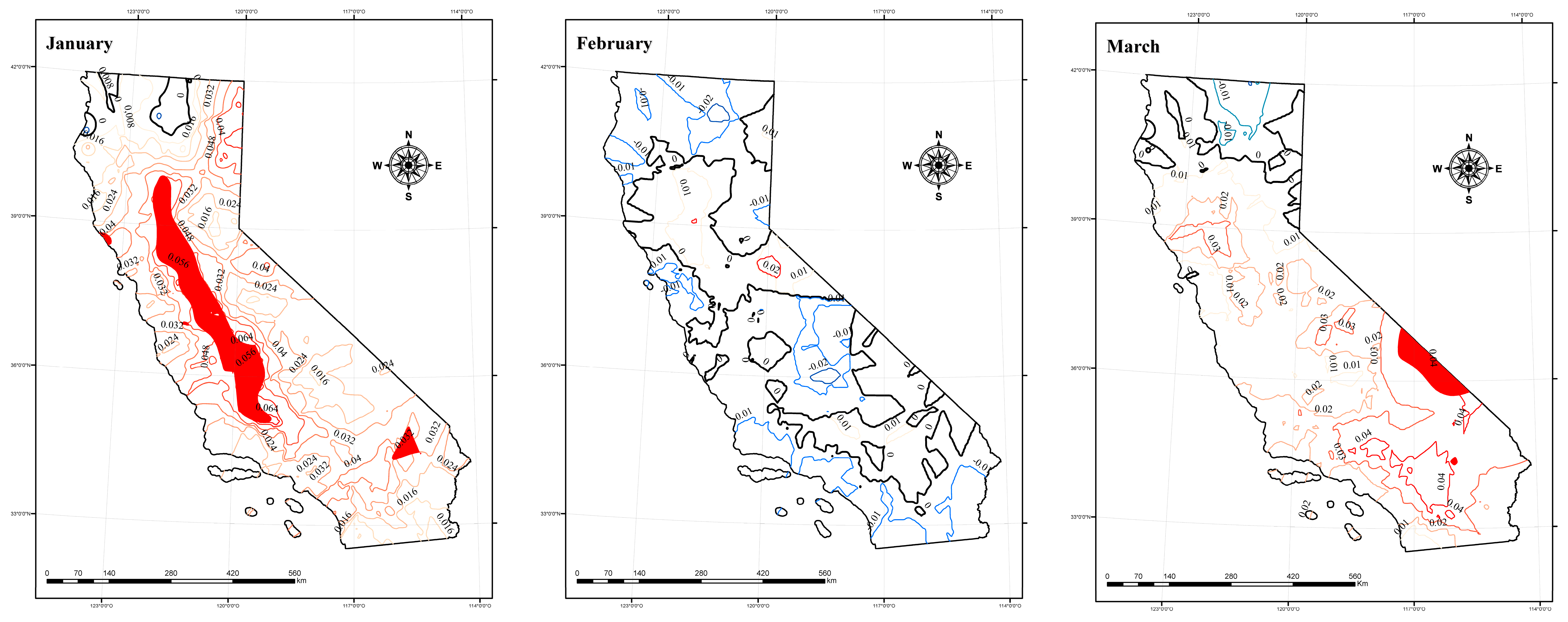
On the monthly scale, the strongest average warming is found in November at +0.04 °C/year. January, July, August and November are the months with the highest fraction (25–38%) of significant trends at the individual stations.

-

The coastal cooling effect in summer gives a trend around zero value, contrary to the results of previous research conducted for this season in different time periods.

-

As regards the teleconnection patterns, Pacific Decadal Oscillation (PDO) has a positive correlation with average temperatures during the period studied, particularly in coastal areas such as Los Angeles, San Francisco and Monterey. In addition, the highest negative correlations with statistical significance have been noted for the West Pacific Oscillation (WPO) from December to April. Moreover, PDO, WPO, NAO, PNA and EPO are the teleconnection patterns that have shown the highest positive correlation from February to May and might have explanatory potential in mean temperature over those months.

-

The Madden–Julian Oscillation (RMM2) is positively correlated with temperature in January and November, with 41.3% of stations have shown a positive correlation in the latter. In November, both EPO and RMM2 have been positively correlated with temperature.

-

On the contrary, Antarctic Oscillation (AAO) and Arctic Oscillation patterns (AO) are unlikely to show great influence on average temperature trends in California.

Further investigations on relationships between teleconnection patterns and climate variables are essential to establish cause–effect relationships that help us to predict future changes in average temperatures in California. Knowledge of atmospheric teleconnections provides us with the opportunity to assess interconnection on a planetary scale.

Knowing the temperature trends recently occurring in the state of California and the influence of teleconnection patterns on them could help policymakers to implement measures in order to mitigate the possible effects caused by global warming. In that line, the authors consider that this research can contribute to advance that knowledge.

References

1. Chervenkov, H.; Slavov, K. Theil–Sen Estimator vs. Ordinary Least Squares—Trend Analysis for Selected ETCCDI Climate Indices. Comptes Rendus L’Academie Bulg. Sci. 2019, 72, 47–54. [Google Scholar] [CrossRef]
2. Vicente-Serrano, S.M.; Quiring, S.M.; Peña-Gallardo, M.; Yuan, S.; Domínguez-Castro, F. A Review of Environmental Droughts: Increased Risk under Global Warming? Earth-Sci. Rev. 2020, 201, 102953. [Google Scholar] [CrossRef]
3. Stillman, J.H. Heat Waves, the New Normal: Summertime Temperature Extremes Will Impact Animals, Ecosystems, and Human Communities. Physiology 2019, 34, 86–100. [Google Scholar] [CrossRef] [PubMed]
4. Haines, A.; Ebi, K. The Imperative for Climate Action to Protect Health. N. Engl. J. Med. 2019, 380, 263–273. [Google Scholar] [CrossRef]
5. Pumo, D.; Noto, L.V. Exploring the Linkage between Dew Point Temperature and Precipitation Extremes: A Multi-Time-Scale Analysis on a Semi-Arid Mediterranean Region. Atmos. Res. 2021, 254, 105508. [Google Scholar] [CrossRef]
6. Hansen, J.; Ruedy, R.; Sato, M.; Lo, K. Global Surface Temperature Change. Rev. Geophys. 2010, 48, RG4004. [Google Scholar] [CrossRef] [Green Version]
7. Masson-Delmotte, V.; Pirani, S.L.; Connors, C.; Péan, S.; Berger, N.; Caud, Y.; Chen, L.; Goldfarb, M.I.; Gomis, M.; Huang, K.; et al. Climate Change 2021: The Physical Science Basis. Contribution of Working Group I to the Sixth Report of the Intergovernmental Panel on Climate Change; Cambridge University Press: Cambridge, UK; New York, NY, USA, 2021; in press. [Google Scholar]
8. Hartmann, D.L.; Tank, A.M.G.K.; Rusticucci, M. IPCC Fifth Assessment Report, Climate Change 2013: The Physical Science Basis. IPCC 2013, AR5, 31–39. [Google Scholar] [CrossRef]
9. Lobell, D.B.; Bonfils, C. The Effect of Irrigation on Regional Temperatures: A Spatial and Temporal Analysis of Trends in California, 1934-2002. J. Clim. 2008, 21, 2063–2071. [Google Scholar] [CrossRef]
10. DeGaetano, A.T.; Allen, R.J. Trends in Twentieth-Century Temperature Extremes across the United States. J. Clim. 2002, 15, 3188–3205. [Google Scholar] [CrossRef]
11. Hamlet, A.F.; Mote, P.W.; Clark, M.P.; Lettenmaier, D.P. Effects of Temperature and Precipitation Variability on Snowpack Trends in the Western United States. J. Clim. 2005, 18, 4545–4561. [Google Scholar] [CrossRef]
12. Martinez, C.J.; Maleski, J.J.; Miller, M.F. Trends in Precipitation and Temperature in Florida, USA. J. Hydrol. 2012, 452–453, 259–281. [Google Scholar] [CrossRef]
13. Powell, E.J.; Keim, B.D. Trends in Daily Temperature and Precipitation Extremes for the Southeastern United States: 1948–2012. J. Clim. 2015, 28, 1592–1612. [Google Scholar] [CrossRef]
14. Vanos, J.K.; Kalkstein, L.S.; Sanford, T.J. Detecting Synoptic Warming Trends across the US Midwest and Implications to Human Health and Heat-Related Mortality. Int. J. Climatol. 2015, 35, 85–96. [Google Scholar] [CrossRef]
15. Wartenburger, R.; Hirschi, M.; Donat, M.G.; Greve, P.; Pitman, A.J.; Seneviratne, S.I. Changes in Regional Climate Extremes as a Function of Global Mean Temperature: An Interactive Plotting Framework. Geosci. Model Dev. 2017, 10, 3609–3634. [Google Scholar] [CrossRef] [Green Version]
16. Di Luca, A.; de Elía, R.; Bador, M.; Argüeso, D. Contribution of Mean Climate to Hot Temperature Extremes for Present and Future Climates. Weather Clim. Extrem. 2020, 28, 100255. [Google Scholar] [CrossRef]
17. Davey, C.A.; Pielke, R.A. Microclimate Exposures of Surface-Based Weather Stations. Bull. Am. Meteorol. Soc. 2005, 86, 497–504. [Google Scholar] [CrossRef] [Green Version]
18. Cordero, E.C.; Kessomkiat, W.; Abatzoglou, J.; Mauget, S.A. The Identification of Distinct Patterns in California Temperature Trends. Clim. Change 2011, 108, 357–382. [Google Scholar] [CrossRef]
19. LaDochy, S.; Medina, R.; Patzert, W. Recent California Climate Variability: Spatial and Temporal Patterns in Temperature Trends. Clim. Res. 2007, 33, 159–169. [Google Scholar] [CrossRef] [Green Version]
20. Swain, D.L.; Horton, D.E.; Singh, D.; Diffenbaugh, N.S. Trends in Atmospheric Patterns Conducive to Seasonal Precipitation and Temperature Extremes in California. Sci. Adv. 2016, 2, e1501344. [Google Scholar] [CrossRef] [Green Version]
21. Reed, D.D. Historical Temperature Trends in Los Angeles County. Master’s Thesis, University of Southern California, Los Angeles, CA, USA, 2015. [Google Scholar]
22. Sheridan, S.C. North American Weather-Type Frequency and Teleconnection Indices. Int. J. Climatol. 2003, 23, 27–45. [Google Scholar] [CrossRef]
23. Ge, Y.; Gong, G. North American Snow Depth and Climate Teleconnection Patterns. J. Clim. 2009, 22, 217–233. [Google Scholar] [CrossRef] [Green Version]
24. Bayr, T.; Domeisen, D.I.V.; Wengel, C. The Effect of the Equatorial Pacific Cold SST Bias on Simulated ENSO Teleconnections to the North Pacific and California. Clim. Dyn. 2019, 53, 3771–3789. [Google Scholar] [CrossRef]
25. Franzke, C.; Feldstein, S.B.; Lee, S. Synoptic Analysis of the Pacific-North American Teleconnection Pattern. Q. J. R. Meteorol. Soc. 2011, 137, 329–346. [Google Scholar] [CrossRef] [Green Version]
26. Mamalakis, A.; Yu, J.Y.; Randerson, J.T.; Aghakouchak, A.; Foufoula-Georgiou, E. A New Interhemispheric Teleconnection Increases Predictability of Winter Precipitation in Southwestern US. Nat. Commun. 2018, 9, 2332. [Google Scholar] [CrossRef] [Green Version]
27. Yu, B.; Lin, H.; Soulard, N. A Comparison of North American Surface Temperature and Temperature Extreme Anomalies in Association with Various Atmospheric Teleconnection Patterns. Atmosphere 2019, 10, 172. [Google Scholar] [CrossRef] [Green Version]
28. Zhou, W.; Yang, D.; Xie, S.-P.; Ma, J. Amplified Madden–Julian Oscillation Impacts in the Pacific–North America Region. Nat. Clim. Chang. 2020, 10, 654–660. [Google Scholar] [CrossRef]
29. Leathers, D.J.; Yarnal, B.; Palecki, M.A. The Pacific/North American Teleconnection Pattern and United States Climate. Part I: Regional Temperature and Precipitation Associations. J. Clim. 1991, 4, 517–528. [Google Scholar] [CrossRef]
30. Baxter, S.; Nigam, S. Key Role of the North Pacific Oscillation-West Pacific Pattern in Generating the Extreme 2013/14 North American Winter. J. Clim. 2015, 28, 8109–8117. [Google Scholar] [CrossRef] [Green Version]
31. Lee, Y.Y.; Grotjahn, R. Evidence of Specific MJO Phase Occurrence with Summertime California Central Valley Extreme Hot Weather. Adv. Atmos. Sci. 2019, 36, 589–602. [Google Scholar] [CrossRef] [Green Version]
32. Macdonald, G.M.; Moser, K.A.; Bloom, A.M.; Potito, A.P.; Porinchu, D.F.; Holmquist, J.R.; Hughes, J.; Kremenetski, K.V. Prolonged California Aridity Linked to Climate Warming and Pacific Sea Surface Temperature. Sci. Rep. 2016, 6, 33325. [Google Scholar] [CrossRef] [Green Version]
33. Schulte, J. Continuum-based Teleconnection Indices of United States Wintertime Temperature Variability. Int. J. Climatol. 2021, 41, E3122–E3141. [Google Scholar] [CrossRef]
34. Trouet, V.; Taylor, A.H.; Carleton, A.M.; Skinner, C.N. Interannual Variations in Fire Weather, Fire Extent, and Synoptic-Scale Circulation Patterns in Northern California and Oregon. Theor. Appl. Climatol. 2009, 95, 349–360. [Google Scholar] [CrossRef] [Green Version]
35. Barnston, A.G.; Livezey, R.E.; Halpert, M.S. Modulation of Southern Oscillation-Northern Hemisphere Mid-Winter Climate Relationships by the QBO. J. Clim. 1991, 4, 203–217. [Google Scholar] [CrossRef] [Green Version]
36. Wallace, J.; Gutzler, D. Teleconnections in the Geopotential Height Field during the Northern Hemisphere Winter. Mon. Weather Rev. Am. Meteorol. Soc. 1981, 109, 784–812. [Google Scholar] [CrossRef]
37. Goodrich, G.B. Influence of the Pacific Decadal Oscillation on Winter Precipitation and Drought during Years of Neutral ENSO in the Western United States. Weather Forecast. 2007, 22, 116–124. [Google Scholar] [CrossRef]
38. Ropelewski, C.F.; Halpert, M.S. North American Precipitation and Temperature Patterns Associated with the El Niño/Southern Oscillation (ENSO). Mon. Weather Rev. 2002, 114, 2352–2362. [Google Scholar] [CrossRef] [Green Version]
39. Guirguis, K.; Gershunov, A.; Shulgina, T.; Clemesha, R.E.S.; Ralph, F.M. Atmospheric Rivers Impacting Northern California and Their Modulation by a Variable Climate. Clim. Dyn. 2019, 52, 6569–6583. [Google Scholar] [CrossRef] [Green Version]
40. Mills, C.M.; Walsh, J.E. Seasonal Variation and Spatial Patterns of the Atmospheric Component of the Pacific Decadal Oscillation. J. Clim. 2013, 26, 1575–1594. [Google Scholar] [CrossRef]
41. Velasco, E.M.; Gurdak, J.J.; Dickinson, J.E.; Ferré, T.P.A.; Corona, C.R. Interannual to Multidecadal Climate Forcings on Groundwater Resources of the U.S. West Coast. J. Hydrol. Reg. Stud. 2017, 11, 250–265. [Google Scholar] [CrossRef] [Green Version]
42. Roksvåg, T.; Lutz, J.; Grinde, L.; Dyrrdal, A.V.; Thorarinsdottir, T.L. Consistent Intensity-Duration-Frequency Curves by Post-Processing of Estimated Bayesian Posterior Quantiles. J. Hydrol. 2021, 603, 127000. [Google Scholar] [CrossRef]
43. Dettinger, M.D.; Ralph, F.M.; Das, T.; Neiman, P.J.; Cayan, D.R. Atmospheric Rivers, Floods and the Water Resources of California. Water 2011, 3, 445–478. [Google Scholar] [CrossRef]
44. Allen, R.J.; Luptowitz, R. El Niño-like Teleconnection Increases California Precipitation in Response to Warming. Nat. Commun. 2017, 8, 16055. [Google Scholar] [CrossRef] [PubMed]
45. Jones, C. Occurrence of Extreme Precipitation Events in California and Relationships with the Madden-Julian Oscillation. J. Clim. 2000, 13, 3576–3587. [Google Scholar] [CrossRef]
46. Luteyn, J.L.; Hickman, J.C. The Jepson Manual: Higher Plants of California; University of California Press: Berkeley, CA, USA, 1993; ISBN 0-520-082559. [Google Scholar]
47. Pathak, T.; Maskey, M.; Dahlberg, J.; Kearns, F.; Bali, K.; Zaccaria, D. Climate Change Trends and Impacts on California Agriculture: A Detailed Review. Agronomy 2018, 8, 25. [Google Scholar] [CrossRef] [Green Version]
48. Killam, D.; Bui, A.; LaDochy, S.; Ramirez, P.; Willis, J.; Patzert, W. California Getting Wetter to the North, Drier to the South: Natural Variability or Climate Change? Climate 2014, 2, 168–180. [Google Scholar] [CrossRef] [Green Version]
49. Center, W.R.C. Western Regional Climate Center. In WRCC; Tuweep, Arizona Stn. Report; 2000; Available online: https://wrcc.dri.edu/ (accessed on 16 February 2021).
50. He, M.; Gautam, M. Variability and Trends in Precipitation, Temperature and Drought Indices in the State of California. Hydrology 2016, 3, 14. [Google Scholar] [CrossRef] [Green Version]
51. Ríos Cornejo, D.; Penas, Á.; Álvarez-Esteban, R.; del Río, S. Links between Teleconnection Patterns and Mean Temperature in Spain. Theor. Appl. Climatol. 2015, 122, 1–18. [Google Scholar] [CrossRef]
52. Thom, H.C.S. Some Methods of Climatological Analysis; Secretariat of the World Meteorological Organization: Geneva, Switzerland, 1966. [Google Scholar]
53. Del Río, S.; Anjum Iqbal, M.; Cano-Ortiz, A.; Herrero, L.; Hassan, A.; Penas, A. Recent Mean Temperature Trends in Pakistan and Links with Teleconnection Patterns. Int. J. Climatol. 2013, 33, 277–290. [Google Scholar] [CrossRef]
54. Sarricolea, P.; Meseguer-Ruiz, Ó.; Serrano-Notivoli, R.; Soto, M.V.; Martin-Vide, J. Trends of Daily Precipitation Concentration in Central-Southern Chile. Atmos. Res. 2019, 215, 85–98. [Google Scholar] [CrossRef]
55. Hijmans, A.R.J.; Phillips, S.; Leathwick, J.; Elith, J.; Hijmans, M.R.J. Dismo: Species Distribution Modeling. 2021. Available online: https://cran.r-project.org/web/packages/dismo/dismo.pdf (accessed on 10 September 2020).
56. Kukal, M.; Irmak, S. Long-Term Patterns of Air Temperatures, Daily Temperature Range, Precipitation, Grass-Reference Evapotranspiration and Aridity Index in the USA Great Plains: Part I. Spatial Trends. J. Hydrol. 2016, 542, 953–977. [Google Scholar] [CrossRef] [Green Version]
57. Peña-Angulo, D.; Gonzalez-Hidalgo, J.C.; Sandonís, L.; Beguería, S.; Tomas-Burguera, M.; López-Bustins, J.A.; Lemus-Canovas, M.; Martin-Vide, J. Seasonal Temperature Trends on the Spanish Mainland: A Secular Study (1916–2015). Int. J. Climatol. 2021, 41, 3071–3084. [Google Scholar] [CrossRef]
58. Yue, S.; Wang, C.Y. The Mann-Kendall Test Modified by Effective Sample Size to Detect Trend in Serially Correlated Hydrological Series. Water Resour. Manag. 2004, 18, 201–218. [Google Scholar] [CrossRef]
59. Gocic, M.; Trajkovic, S. Analysis of Changes in Meteorological Variables Using Mann-Kendall and Sen’s Slope Estimator Statistical Tests in Serbia. Glob. Planet. Chang. 2013, 100, 172–182. [Google Scholar] [CrossRef]
60. Karmeshu, N. Trend Detection in Annual Temperature & Precipitation Using the Mann Kendall Test—A Case Study to Assess Climate Change on Select States in the Northeastern United States. Master’s Thesis, University of Pennsylvania, Philadelphia, PA, USA, 2015. [Google Scholar]
61. Song, X.; Zhang, J.; Zou, X.; Zhang, C.; AghaKouchak, A.; Kong, F. Changes in Precipitation Extremes in the Beijing Metropolitan Area during 1960–2012. Atmos. Res. 2019, 222, 134–153. [Google Scholar] [CrossRef]
62. Patakamuri, S.K.; O’Brien, N. Modifiedmk: Modified Mann Kendall Trend Tests. 2020. Available online: https://www.researchgate.net/publication/348231702_Modifiedmk_Modified_Mann_Kendall_Trend_Tests (accessed on 6 July 2020).
63. Liu, Q.; Shepherd, B.; Li, C. Presiduals: An R Package for Residual Analysis Using Probability-Scale Residuals. J. Stat. Softw. 2020, 94, 1–27. [Google Scholar] [CrossRef]
64. ArcGIS Desktop: Release 10.8; Environmental Systems Research Institute: Redlands, CA, USA, 2019.
65. Barber, X.; Conesa, D.; López-Quílez, A.; Mayoral, A.; Morales, J.; Barber, A. Bayesian Hierarchical Models for Analysing the Spatial Distribution of Bioclimatic Indices. Sort 2017, 41, 277–296. [Google Scholar] [CrossRef]
66. Gribov, A.; Krivoruchko, K. Empirical Bayesian Kriging Implementation and Usage. Sci. Total Environ. 2020, 722, 137290. [Google Scholar] [CrossRef]
67. Krivoruchko, K. Empirical Bayesian Kriging. ESRI Press 2012, 2012, 6–10. [Google Scholar]
68. Newman, M.; Alexander, M.A.; Ault, T.R.; Cobb, K.M.; Deser, C.; Di Lorenzo, E.; Mantua, N.J.; Miller, A.J.; Minobe, S.; Nakamura, H.; et al. The Pacific Decadal Oscillation, Revisited. J. Clim. 2016, 29, 4399–4427. [Google Scholar] [CrossRef] [Green Version]
69. Christy, J.R.; Norris, W.B.; Redmond, K.; Gallo, K.P. Methodology and Results of Calculating Central California Surface Temperature Trends: Evidence of Human-Induced Climate Change? J. Clim. 2006, 19, 548–563. [Google Scholar] [CrossRef] [Green Version]
70. Niles, M.T.; Mueller, N.D. Farmer Perceptions of Climate Change: Associations with Observed Temperature and Precipitation Trends, Irrigation, and Climate Beliefs. Glob. Environ. Chang. 2016, 39, 133–142. [Google Scholar] [CrossRef] [Green Version]
71. Fassnacht, S.R.; López-Moreno, J.I.; Ma, C.; Weber, A.N.; Pfohl, A.K.D.; Kampf, S.K.; Kappas, M. Spatio-Temporal Snowmelt Variability across the Headwaters of the Southern Rocky Mountains. Front. Earth Sci. 2017, 11, 505–514. [Google Scholar] [CrossRef]
72. Guarín, A.; Taylor, A.H. Drought Triggered Tree Mortality in Mixed Conifer Forests in Yosemite National Park, California, USA. For. Ecol. Manag. 2005, 218, 229–244. [Google Scholar] [CrossRef]
73. Hayhoe, K.; Cayan, D.; Field, C.B.; Frumhoff, P.C.; Maurer, E.P.; Miller, N.L.; Moser, S.C.; Schneider, S.H.; Cahill, K.N.; Cleland, E.E.; et al. Emissions Pathways, Climate Change, and Impacts on California. Proc. Natl. Acad. Sci. USA 2004, 101, 12422–12427. [Google Scholar] [CrossRef] [PubMed] [Green Version]
74. Trenberth, K.E. The Impact of Climate Change and Variability on Heavy Precipitation, Floods, and Droughts. In Encyclopedia of Hydrological Sciences; John Wiley & Sons Ltd.: London, UK, 2005; Available online: https://www.researchgate.net/publication/227555971_The_Impact_of_Climate_Change_and_Variability_on_Heavy_Precipitation_Floods_and_Droughts (accessed on 2 May 2022).
75. Williams, A.P.; Seager, R.; Abatzoglou, J.T.; Cook, B.I.; Smerdon, J.E.; Cook, E.R. Contribution of Anthropogenic Warming to California Drought during 2012-2014. Geophys. Res. Lett. 2015, 42, 6819–6828. [Google Scholar] [CrossRef] [Green Version]
76. Weiss-Penzias, P.S.; Bank, M.S.; Clifford, D.L.; Torregrosa, A.; Zheng, B.; Lin, W.; Wilmers, C.C. Marine Fog Inputs Appear to Increase Methylmercury Bioaccumulation in a Coastal Terrestrial Food Web. Sci. Rep. 2019, 9, 17611. [Google Scholar] [CrossRef] [Green Version]
77. Torregrosa, A.; O’brien, T.A.; Faloona, I.C. Coastal Fog, Climate Change, and the Environment. Eos 2014, 95, 473–474. [Google Scholar] [CrossRef] [Green Version]
78. Lebassi, B.; Gonzalez, J.; Fabris, D.; Maurer, E.; Miller, N.; Milesi, C.; Switzer, P.; Bornstein, R. Observed 1970-2005 Cooling of Summer Daytime Temperatures in Coastal California. J. Clim. 2009, 22, 3558–3573. [Google Scholar] [CrossRef] [Green Version]
79. Johnstone, J.A.; Dawson, T.E. Climatic Context and Ecological Implications of Summer Fog Decline in the Coast Redwood Region. Proc. Natl. Acad. Sci. USA 2010, 107, 4533–4538. [Google Scholar] [CrossRef] [Green Version]
80. Tamrazian, A.; Ladochy, S.; Willis, J.; Patzert, W.C. Heat Waves in Southern California: Are They Becoming More Frequent and Longer Lasting? In Yearbook of the Association of Pacific Coast Geographers. Available online: https://climate.nasa.gov/files/LAHeatWaves-JournalArticle.pdf (accessed on 18 June 2021).
81. Basu, R.; Rau, R.; Pearson, D.; Malig, B. Temperature and Term Low Birth Weight in California. Am. J. Epidemiol. 2018, 187, 2306–2314. [Google Scholar] [CrossRef]
82. The California Department of Water Resources. California Climate Science and Data: For Water Resources Management; California Water Library: Sacramento, CA, USA, 2015.
83. Diffenbaugh, N.S.; Swain, D.L.; Touma, D. Anthropogenic Warming Has Increased Drought Risk in California. Proc. Natl. Acad. Sci. USA 2015, 112, 3931–3936. [Google Scholar] [CrossRef] [PubMed] [Green Version]
84. Bellard, C.; Bertelsmeier, C.; Leadley, P.; Thuiller, W.; Courchamp, F. Impacts of Climate Change on the Future of Biodiversity. Ecol. Lett. 2012, 15, 365–377. [Google Scholar] [CrossRef] [PubMed] [Green Version]
85. Wheeler, M.C.; Hendon, H.H. An All-Season Real-Time Multivariate MJO Index: Development of an Index for Monitoring and Prediction. Mon. Weather Rev. 2004, 132, 1917–1932. [Google Scholar] [CrossRef]
86. Dasgupta, P.; Metya, A.; Naidu, C.V.; Singh, M.; Roxy, M.K. Exploring the Long-Term Changes in the Madden Julian Oscillation Using Machine Learning. Sci. Rep. 2020, 10, 18567. [Google Scholar] [CrossRef] [PubMed]
87. Liu, Y.-C.; Di, P.; Chen, S.-H.; Damassa, J. Relationships of Rainy Season Precipitation and Temperature to Climate Indices in California: Long-Term Variability and Extreme Events. J. Clim. 2018, 31, 1921–1942. [Google Scholar] [CrossRef]
88. Barron, J.A.; Anderson, L. Enhanced Late Holocene ENSO/PDO Expression along the Margins of the Eastern North Pacific. Quat. Int. 2011, 235, 3–12. [Google Scholar] [CrossRef] [Green Version]
89. Zhang, N.; Pathak, T.B.; Parker, L.E.; Ostoja, S.M. Impacts of Large-Scale Teleconnection Indices on Chill Accumulation for Specialty Crops in California. Sci. Total Environ. 2021, 791, 148025. [Google Scholar] [CrossRef]
90. Alfaro, E.; Gershunov, A.; Cayan, D.; Steinemann, A.; Pierce, D.; Barnett, T. A Method for Prediction of California Summer Air Surface Temperature. Eos 2004, 85, 553–558. [Google Scholar] [CrossRef] [Green Version]
91. Zheng, C.; Chang, E.K.M.; Kim, H.M.; Zhang, M.; Wang, W. Impacts of the Madden-Julian Oscillation on Storm-Track Activity, Surface Air Temperature, and Precipitation over North America. J. Clim. 2018, 31, 6113–6134. [Google Scholar] [CrossRef]
92. Gong, D.; Wang, S. Definition of Antarctic Oscillation Index. Geophys. Res. Lett. 1999, 26, 459–462. [Google Scholar] [CrossRef] [Green Version]
Figure 1. California physical map and meteorological stations analysed ().
Applsci 12 05831 g001
Figure 2. Percentages of meteorological stations with positive and negative trends.
Applsci 12 05831 g002
Figure 3. Spatial distribution trends (positive in red, negative in blue) in mean temperatures (°C/year) and their statistical significance on monthly, seasonal and annual time-scale. Area with positive statistical significance at 95% confidence level.
Applsci 12 05831 g003aApplsci 12 05831 g003bApplsci 12 05831 g003cApplsci 12 05831 g003dApplsci 12 05831 g003eApplsci 12 05831 g003f
Figure 4. Heatmap with the percentage of meteorological stations that have shown statistical significance positive (+) or negative () correlations between teleconnection patterns and average temperatures at 95% confidence level. Blank spaces are zero percentage values that had been removed to ease visualization. The top histogram (blue) represents the percentage contribution of the teleconnection patterns to the variance of temperature of the meteorological stations in each month. The right histogram (green) shows the percentage contribution of each teleconnection pattern for itself, in the whole year. PDO (Pacific Decadal Oscillation), PNA (Pacific–North American), WPO (Western Pacific Oscillation), EPO (East Pacific Oscillation), NAO (North Atlantic Oscillation), ENSO (El Niño–Southern Oscillation), RMM1 and RMM2 (Real Multivariate MJO), AO (Artic Oscillation) and AAO (Antarctic Oscillation).
Applsci 12 05831 g004
Figure 5. Percentage of meteorological stations in the State of California with significant correlations (positive in red, negative in blue) between PDO and temperature.
Applsci 12 05831 g005
Figure 6. Percentage of meteorological stations in the State of California with significant correlations (positive in red, negative in blue) between PNA and temperature.
Applsci 12 05831 g006
Figure 7. Percentage of meteorological stations in the State of California with significant correlations (positive in red, negative in blue) between WPO and temperature.
Applsci 12 05831 g007
Figure 8. Percentage of meteorological stations in the State of California with significant correlations (positive in red, negative in blue) between EPO and temperature.
Applsci 12 05831 g008
Figure 9. Percentage of meteorological stations in the State of California with significant correlations (positive in red, negative in blue) between NAO and temperature.
Applsci 12 05831 g009
Figure 10. Percentage of meteorological stations in the State of California with significant correlations (positive in red, negative in blue) between ENSO and temperature.
Applsci 12 05831 g010
Figure 11. Percentage of meteorological stations in the State of California with significant correlations (positive in red, negative in blue) between RMM1 index of MJO and temperature.
Applsci 12 05831 g011
Figure 12. Percentage of meteorological stations in the State of California with significant correlations (positive in red, negative in blue) between RMM2 index of MJO and temperature.
Applsci 12 05831 g012