Abstract
As the core process of case-based reasoning (CBR), case retrieval is the foundation for CBR success, and the quality of case retrieval depends on the case similarity measure. We improved the CBR system for aeroengine fault diagnosis by embedding the attitudinal Choquet integral (ACI) and 2-order additive measure to consider attribute interactions and decision makers’ attitudes. The enhanced case retrieval method can not only integrate the local similarity, attribute importance, and interaction between attributes, but also incorporate the attitude of the decision maker, thus producing more comprehensive and reasonable global similarity and high-quality recommendations. An experimental study of aeroengine fault diagnosis and comparisons with other similarity aggregation methods were performed to demonstrate the effectiveness of the proposed method.
1. Introduction
When faced with a new problem, it is always helpful to consider the solution to a similar problem from the past. From increasing historical experience, it is possible to identify useful solutions. Case-based reasoning (CBR), a knowledge-based system, is an experience-based method [1]. It solves new problems by retrieving the most similar case from a member of cases [2], which is also the core process of the CBR cycle [3]. CBR is demonstrably suitable for solving problems in fault diagnosis. Yang et al. (2004) added a Petri net to a CBR system to improve the revision function, and successfully applied it to electronic motor diagnosis [4]. Owing to the complexity and uncertainty of the operating environment, Yang et al. (2017) proposed an optimized hybrid model combining CBR and a Bayesian network for embedded software fault diagnosis [5]. A CBR system for the intelligent fault diagnosis of power equipment was proposed by Ma [6].
Decision makers often need to weigh different criteria when making decisions as the factors involved in decision making become more complex. In addition, the importance of different criteria should be considered. Multi-attribute decision making (MADM), or multi-criteria decision making (MCDM), is a decision making methodological framework based on multiple criteria or multiple attributes [7]. MADM provides decision makers with a set of recommendations for alternatives, goals, or solutions [8]. The main task of MADM is to assess a member of the alternatives and then rank them [9,10]. MCDM has been applied in many fields such as supplier [11], material [12], and flotation machine selections [13].
Evidently, MADM and CBR have some commonalities. Both can solve the problem of choosing the best solution from among numerous alternatives [14]. On the one hand, CBR is good at dealing with knowledge-intensive and multidisciplinary complex problems, such as medical diagnosis and aviation fault diagnosis. In general, fault diagnosis in these domains cannot be achieved simply by searching for a few keywords. In most cases, a detailed description of the fault is required. Therefore, it may be more reasonable to consider the semantics of fault descriptions rather than strings. In addition, there are several complex unstructured problems in these domains. Some similarity retrieval methods used in CBR can solve these problems. On the other hand, MADM can provide decision makers with a ranking of alternatives and suggest the best solution. To select the optimal solution among multiple solutions, the trade-offs between different attributes and the weight of each attribute must be considered in the MADM. Thus, integrating CBR with MADM can not only deal with complex problems in some fields, but also consider the weights of multiple attributes, thus improving the accuracy of CBR. In view of this, Alptekin and Büyüközkan (2011) combined AHP with CBR to build an intelligent tourism system [14], Malekpoor et al. (2018) proposed a TOPSIS-CBR approach for cancer therapy and successfully tested it using real datasets [15], and Berman et al. (2015) proposed a hybrid approach to select construction materials in mechanical engineering [16].
However, two defects exist in the aforementioned studies. First, in most cases, the interactions among decision attributes were ignored; that is, different attributes were assumed to be noninteractive or independent of each other. In fact, there are positive or negative interactions between certain attributes that cannot be ignored [17]. Therefore, nonadditive measures should be introduced to remedy this defect. In addition, when synthesizing the importance and interaction of attributes, few studies have considered the influence of decision makers’ attitudes on the decision making process. Aggarwal (2017, 2018) believes that the attitude of decision makers may be the reason why many classical operators do not work in the process of human aggregation, and there are three basic elements that need to be considered in the decision making process: the initial weight of attributes, interaction between attributes, and the attitude of decision makers [18,19]. In decision making, the reliability of alternatives is usually derived from human decision behavior [20]. The model based on ACI can effectively model human decision behavior by considering the preference information of decision makers, which has been applied in the fields of decision making, assessment, and preference learning in recent years [21,22,23].
In this study, an improved case retrieval method is proposed to remedy the shortcomings of the most critical case similarity measure in the existing CBR system for aeroengine fault diagnosis, that is, attribute weight, attribute interaction and decision maker’s attitude are not considered. Specifically, our improvement includes three aspects: (1) the best–worst method (BWM) for MADM is adopted to determine the initial weights of attributes. (2) An approximation of non-additive measures, the 2-order additive measure, is used to consider different interaction relationships between attributes, including positive, independent, and negative interactions. (3) The ACI is exploited to integrate the local similarities associated with different attribute categories, the non-additive measure related to attribute interaction, and the preference depending on decision maker’s attitude to obtain the global similarity.
The remainder of this paper is organized as follows. Section 2 reviews the relevant literature. In Section 3, the preliminary knowledge is presented. Section 4 describes the method and process of CBR for aeroengine fault diagnosis, including three local similarity measures associated with different attribute types, a 2-order additive measure considering the interaction between attributes, and a global similarity measure based on ACI. In Section 5, an experimental study on the proposed retrieval method in aeroengine fault diagnosis is performed. Finally, in Section 6, we summarize our main conclusions and discuss future research directions.
2. Literature Review
2.1. Fault Diagnosis of Aeroengines
As one of the most complicated structures of aircraft, aeroengines work in extremely harsh environments of high temperature, high pressure, and strong vibration for a long time, leading to fatigue, creep, fracture, and many other component failures. Therefore, fault diagnosis of aeroengines is necessary to ensure safe and efficient operation of the engine. There are three widely used methods for aeroengine fault diagnosis: model-based, knowledge-based, and statistical learning methods.
Model-based fault diagnosis needs to analyze the entire structure of mechanical equipment and establish corresponding mathematical or simulation models. Peng et al. (2018) established a simulation model for lubricating oil systems [24]. Using this model, an online fault diagnosis system was built using the parameter trend analysis method. Kim and Mylaraswamy (2006) developed a fault diagnosis and prediction system based on discrete event system modeling and tested the system using actual flight data of startup component failures [25]. They believed that such qualitative modeling methods can be applied to the hierarchical diagnosis of complex large-scale systems because they do not require a detailed model of the system. Wang et al. (2018) established a nonlinear model for the fault diagnosis of a fuel regulator using a particle swarm optimization algorithm combined with a back-propagation neural network for higher diagnosis precision [26]. The nonlinear modeling method is closer to the real operating state of an aeroengine with higher modeling accuracy. This type of method, combined with some conventional fault classification algorithms, can better serve the fault diagnosis of aeroengines.
Knowledge-based fault diagnosis can effectively utilize expert knowledge and experience to make judgments without relying on analytical mathematical models. An expert system is the most classic knowledge-based fault-diagnosis method. Sun et al. (2021) proposed an expert system for aeroengine gas-path fault diagnosis to manage the flight data of various types of engines [27]. Chen, Qu, and Fang (2022) built the first tentative case base in the field of aeroengine fault diagnosis, and developed a CBR system with a highly accurate novel similarity measure for fault diagnosis of aeroengines, where three local similarity measures associated with different attributes were integrated [28].
Statistical learning methods for the fault diagnosis of aeroengines mainly include neural networks, support vector machines, and Bayesian networks. Zhao et al. (2020) used neural network methods such as convolutional neural networks and back-propagation neural networks for aeroengine gas-path fault diagnosis instead of traditional thermodynamic methods [29]. Neural networks can not only obtain higher accuracy of fault diagnosis but also have better adaptability to aeroengine data. Romessis and Mathioudakis (2004) proposed a Bayesian belief network for gas turbine performance fault diagnosis, which can be built from mathematical models rather than hard-to-obtain flight data from malfunctioning operations [30].
2.2. Nonadditive Measure
Mathematically, a measure is a function that assigns a number to a subset of a set. This number can be compared with the size, volume, probability, etc. The characteristic of classical measures is additivity. For example, the probability of several mutually exclusive events is the sum of the probability of each event. However, in certain cases, the additive measure does not satisfy this requirement. For example, the work efficiency of two people is not simply the sum of their work efficiency. Similarly, in CBR, interactions may exist between attributes, indicating that attributes are not always independent of each other. Therefore, the combined weight of two interactive attributes is not always the sum of the weights of the two attributes.
In response to the above violation of additivity, Choquet (1954) [31] and Sugeno (1974) [32] proposed nonadditive measures, namely fuzzy measures, which were, respectively, the Choquet and Sugeno integrals. These two nonadditive measures have a wide range of applications, particularly in MCDM situations [33]. The MCDM with fuzzy measures can not only fully consider the relative weight of the decision criteria, but also flexibly describe the interaction between criteria [34]. However, with an increase in parameters, the complexity of the nonadditive measure increases exponentially, which is one of the defects of the fuzzy measure. For example, when the cardinality of set X is n, the values of n parameters must be determined for additive measures; for a nonadditive measure, we must compute the values of all subsets of X with 2n parameters. To address the complexity of the model, many other nonadditive measures have been proposed, such as λ-addition fuzzy measures [35], in which only n − 1 parameters are required. However, λ-addition fuzzy measures also have some disadvantages. For nonadditive measures, there are three types of interactions: independent, redundant, and complementary. In the λ-addition fuzzy measure model, only one interaction exists [36].
Grabisch (1997) [37] proposed an additive discrete fuzzy measure of order k. The definition of the k-order additive measure is based on the pseudo-Boolean function [38], which is an approximate representation of the k-order nonadditive measure. In addition, the Mobius transformation is used to describe k-order additive measures [39]. The k-order additive measures can not only deal with the complexity of nonadditive measures, but also represent three different types of interactions using Shapley indices as the development of the Shapley value [40]. Many scholars have improved and developed k-order additive measures and applied them in various fields. For example, Honda et al. (2022) developed a k-order additive measure for a nondiscrete case [41]. The 2-order additive measure can solve the contradiction between complexity and precision in a wide range of applications [42]. Zhang et al. (2021) proposed a 2-order additive fuzzy measure based on intuitionistic fuzzy sets to quantitatively evaluate the interactions between attributes [43]. Li et al. (2016) proposed a simulation credibility group evaluation method using 2-order additive fuzzy measure to train a traction-drive simulation system [44]. The 2-order additive measure is only concerned with the importance of each attribute and the interaction between two attributes, which is a perfect compromise between the performance and computational complexity of the nonadditive measure, and has been widely used in MADM methods [45].
3. Preliminaries
In this section, we provide three definitions that constitute the basis for subsequent discussion.
Definition 1.
Nonadditive measure [32].
If X is a finite nonempty set, then a set function μ: Γ(X)→ [0, 1] can be defined as a nonadditive measure or fuzzy measure if the set function satisfies the following conditions:
- (i)
- (ii)
where μ is a regular fuzzy measure on X.
Definition 2.
Choquet integral (CI) [31].
Let μ: Γ(X)→ [0, 1] be a nonadditive measure of X; then, the Choquet integral of function F(x) can be defined as
where. is a permutation on set A that satisfies. Note that.
Definition 3.
Attitudinal Choquet integral (ACI) [19].
Let μ: Γ(X)→[0, 1] be a nonadditive measure on X; then, the attitudinal Choquet integral can be defined as
whereindicates the decision maker’s attitude satisfyingand. A higherindicates a more optimistic decision maker. Typically, the value ofis set to 10n [19]. μ refers to the importance of individual attributes and their interactions.
4. Improved Retrieval Method for CBR
4.1. CBR Framework
When a new case appears, a CBR system begins with case retrieval. First, key attributes are extracted to represent the case. Generally, attribute data can be divided into several types. In this study, we propose different similarity measures for three types of attribute data. In addition, for an accurate CBR system, the weights of individual attributes and the interaction between attributes should be considered. Many previous studies calculated the weight of attributes using an average operator or weighted average operator, which may lead to a significant difference between the calculated weights and the actual weights. However, the attribute weights are not the same in most cases. In some cases, attributes are not independent of each other, and the interaction between attributes is too important to ignore. Therefore, the joint weights of multiple attributes are not always the sum of the weights of each attribute. We adopt a 2-order additive measure to elaborate on all interactions between attributes. Furthermore, considering the influence of the decision maker’s attitude, the ACI was used to obtain the global similarity between the two cases. The framework of the proposed CBR system is shown in Figure 1 and elaborated below.
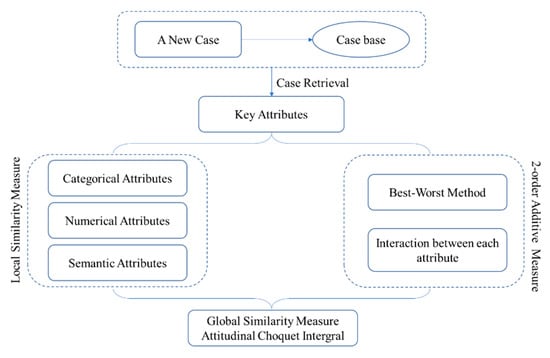
Figure 1.
Framework of the proposed case-based reasoning (CBR) system.
4.2. Local Similarity Measure
In general, there are various data types in CBR systems. In our case base, the data attributes are divided into three types: categorical, numerical, and semantic. Categorical attributes include the aeroengine model, aeroengine category, aeroengine operation state, thrust performance, temperature performance, rotational performance, aeroengine shutdown, and other anomalies. Numerical attributes contain flight height and speed. The semantic attributes contain the fault part and mode in aeroengines. The similarity calculation methods for the three types of data attributes can be found in our previous study [28].
- (1)
- Categorical Attributes.
In our CBR system, the similarity of categorical attributes is calculated using Equation (3).
where is the value of attribute j in new case nc, and is the value of attribute j in case ci. , where I is the total number of cases. , where J is the total number of attributes.
- (2)
- Numerical Attributes.
The similarity between numerical attributes is defined as the normalized distance between two attribute values, calculated using Equations (4) and (5).
where is the value of attribute j in nc, is the value of attribute j in ci, while and represent the maximum and minimum values of attribute j, respectively.
- (3)
- Semantic Attributes.
The semantic similarity based on tree is used to measure the semantic attribute similarity of the aeroengine fault part and fault mode, which defines the association of the fault mode with the fault part. It consists of two elements: tree structure of the fault part and semantic diagram of the fault mode. Figure 2 shows a schematic diagram of the fault part tree structure of an aeroengine, wherein parts are differentiated and structured to calculate their similarities under the same or different fault modes. Further, a fault mode semantic diagram is developed, as shown in Figure 3. Finally, the association of fault mode with fault part is defined by combining the fault part tree structure and the fault mode semantic diagram, as shown in Figure 4.
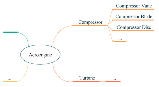
Figure 2.
Tree structure of fault part.
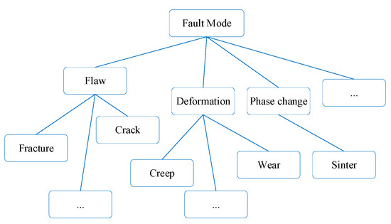
Figure 3.
Semantic diagraph of fault mode.
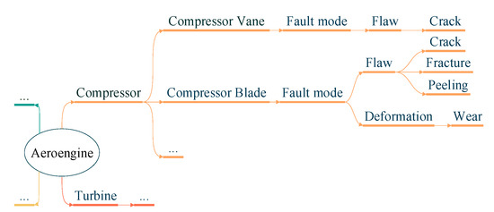
Figure 4.
Aeroengine fault semantic graph.
The measure of semantic similarity is based on the following three constructs.
- (i)
- In the semantic graph, two nodes with shorter distance are more similar than two nodes with longer distance. The shortest path between nodes ni and nj is denoted as Dist (ni, nj). For example, Dist (“Fracture (Compressor Blade)”, “Wear (Compressor Blade)”) = 4 implies that the shortest path between Fracture (Compressor Blade) and Wear (Compressor Blade) is 4.
- (ii)
- The nearest shared parent node nk of nodes ni and nj is represented by Nspn (ni, nj). For example, Nspn (“Crack (Compressor Vane)”, “Crack (Compressor Blade)”) = Compressor, which means compressor is the nearest shared parent node of Crack (Compressor Vane) and Crack (Compressor Blade).
- (iii)
- The distance from a node to the root node is defined as the depth of the node, denoted as Depth(nk). For example, Depth (Compressor Vane) = 2 indicates that the depth of node Compressor Vane from root node Aeroengine is 2.
Then, the semantic similarity is defined as a function of the node location in the taxonomy, which is calculated using Equation (6).
4.3. A 2-Order Additive Measure Method
The main purpose of the proposed method is to determine the range of interaction by combining the weight of each attribute based on the BWM with the degree of interaction between attributes. The maximum entropy principle is then employed to build an optimization model, and finally, the 2-order additive measure is obtained.
First, we present the theoretical basis of the 2-order additive measure. For , a unique 2-order additive measure can be determined when the interaction between attributes satisfies the following conditions [46]:
- (i)
- , , ,where indicates the interaction between and , and indicates the weight of .
- (ii)
- .
- (iii)
- , for both and .
- (iv)
- At least one subset T satisfies , where .
The calculation of the 2-order additive measure comprises the following five progressive operations.
- (1)
- Determine optimal attribute weights by BWM [47].
Step 1. Choose key attributes.
Decision makers must choose key attributes to represent a case. The key attribute set is denoted as .
Step 2. Select the best and the worst attributes among all attributes.
The best attribute usually refers to the most important or considerable attribute, whereas the worst attribute refers to the least important attribute. Notably, if there is more than one best/worst attribute, any can be selected.
Step 3. Compare to other attributes using the numbers 1 through 9.
The decision maker needs to compare the preference of each attribute (except the best one) over in turn. The importance scale is presented in Table 1. The importance ratio vector is denoted as , where denotes the importance ratio of to .

Table 1.
Importance scale.
Step 4. Compare other attributes to using numbers 1 through 9.
Similar to step 3, the preference of other attributes (except the worst one) for is compared in turn. The importance ratio vector is denoted as , where is the importance ratio of to .
Step 5. Compute the optimal weight of each attribute.
Steps 3 and 4 obtain the importance ratio vectors and , which can be regarded as the ratios of weights. Therefore, the importance ratio of to can be expressed as . Similarly, the importance ratio of to is . The optimal weights can be obtained by solving the following optimal model.
Under ideal conditions, the minimum value of the objective function should be 0. Generally, and cannot both be satisfied. Therefore, the logic underlying Model (7) is to search for optimal weights to minimize .
- (2)
- Specify attribute interaction intensity.
According to the above theoretical basis, the interaction between and should satisfy the following inequalities:
The minimum value of the interaction is defined as
Therefore, the value of interaction belongs to the interval . Subsequently, the interval is further divided into t (t is an odd number) subintervals, representing different interaction intensities between attributes, denoted as
Interval indicates that and have no interaction; that is, and are independent of each other. The interval indicates that interaction is negative or redundant, where the interaction intensity of the left term is greater than that of the right term. Interval indicates that interaction is positive or complementary, where the interaction intensity of the left term is less than that of the right term. Let us consider for convenience. Therefore, the interval can be represented as
- (3)
- Determine attribute interaction based on the maximum entropy principle.
Applying the maximum entropy principle, the value of interaction can be obtained by solving the following nonlinear programming problem.
where , , and symbol represents the cardinality of a set.
- (4)
- Determine value of the Mobius representation.
According to the corresponding relationship between the Mobius representation and [48], the value of Mobius can be calculated using Equation (11).
- (5)
- Calculate the 2-order additive measure.
All values of the 2-order additive measure, , are computed using Equation (12).
4.4. Global Similarity
The global similarity between cases is the weighted sum of similarity obtained by integrating the local similarity of different attributes calculated using ACI, as shown in Equation (13).
where . indicates the local similarity considering the three types of similarity calculations with , as explained in Section 4.2. , where is a permutation of that satisfies . Note that . Recall that in ACI, μ describes the importance of individual attributes and their interactions, and λ represents the attitudes of the decision maker.
In the study of Chen et al. (2022) [28], a prototype CBR system for fault diagnosis of aeroengines has been established. However, the system does not consider the weight of attributes, interaction between attributes, and the attitude of decision makers in determining the similarity measure. To address the above defects, this study introduces the 2-order additive measure, an approximation of the nonadditive measure, and ACI to improve the case retrieval method. In particular, the preliminaries presented in Section 3 constitute the theoretical basis of nonadditive measures. The CBR system enhanced with the improved retrieval method can diagnose aeroengine faults more efficiently.
5. Experimental Study and Discussion
This section illustrates the proposed retrieval method using an experimental study. In the experiment, there are four cases of aeroengine fault diagnosis in the case base, as listed in Table 2. The case base is stored in ACCESS software, in which each case is represented by five attributes: the aeroengine model, aeroengine category, aeroengine operation state, other anomalies, and aeroengine fault part and fault mode, denoted by a1, a2, a3, a4, and a5, respectively. Here, a1, a2, a3, a4 are categorical attributes, while a5 is a semantic attribute. Note that in this experiment, we do not cover numerical attributes that are relatively simple and easy to handle. New case information is presented in Table 3. In CBR, the existing cases in the case base must be sorted; therefore, the most similar case is selected to solve the new case.
Table 2.
Four cases in the case base.
Table 3.
A new case for case retrieval.
5.1. Nonadditive Measure Calculation
First, BWM is used to calculate the initial attribute weights. Attribute set A = {a1, a2, a3, a4, a5}. According to the decision maker, a5 is the best attribute (ab) and a2 is the worst attribute (aw). The importance ratios of ab to the other attributes are listed in Table 4, and the importance ratios of other attributes to aw are listed in Table 5.
Table 4.
Importance ratios of ab to other attributes.
Table 5.
Importance ratios of other attributes to aw.
The optimal attribute weights can then be obtained by solving the following optimization problem:
By using MATLAB programming (Version No. R2019b, License No. 40865358, MathWorks, Beijing, China), we have ω1 = 0.0632, ω2 = 0.0465, ω3 = 0.1631, ω4 = 0.3255, ω5 = 0.4018, and the minimum deviation δ = 0.6411. The decision maker’s attitude in Table 4 and Table 5 reveal that the weight relation of the five attributes is . The calculation result is consistent with the decision maker’s attitude.
After obtaining the initial attribute weights, the interactions between attributes must be considered. According to Equation (9), we can get X12 = min (2I1/4, 2I2/4) = min (0.0316, 0.0233) = 0.0233. Here, In refers to ωn. In this experiment study, the attribute number n = 5. Similarly, all values for Xjk are calculated and the results are listed in Table 6.
Table 6.
Values for Xjk.
Second, the interaction interval is divided into subintervals to specify the intensity of the attribute interaction. In the experiment, t = 5. Therefore, the interval is divided into five sub-intervals:
Here, we use K1 to K5 to denote the five subintervals. The decision maker then determines the interaction between any two attributes as a negative/independent/positive relationship. According to the decision maker, the interaction between a1 and a2 is quite negative, thus, the interaction interval between a1 and a2 belongs to K1. Similarly, a1 and a3, a2 and a3 belong to K2; a2 and a4, a2 and a5 belong to K3; a1 and a4, a1 and a5, a3 and a4, a3 and a5 belong to K4; a4 and a5 belongs to K5. Therefore, can be obtained, that is, . Similarly, we can obtain all the interaction intervals for the possible attribute pairs, as listed in Table 7.
Table 7.
Interaction intervals.
Third, based on Model (10), the value of the interaction Ijk can be calculated by solving the following nonlinear programming:
By using MATLAB programming, we obtain all the values of Ijk, as listed in Table 8.
Table 8.
Values for Ijk.
Fourth, the values of Mobius representation can be obtained using Equation (11), as listed in Table 9. For example, .
Table 9.
Values of Mobius representation.
Finally, the 2-order additive measures of all subsets of A are calculated using Equation (12). The results are listed in Table 10. For example, , .
Table 10.
Nonadditive measures of set A.
5.2. Similarity Calculation by ACI
The local similarity between ci and nc can be obtained as shown in Table 11. Recall that a1, a2, a3, and a4 are categorical attributes and a5 is a semantic attribute. Hence, the similarity measures a1, a2, a3, and a4 are calculated using Equation (3), and the similarity measures of a5 are calculated using Equation (6).
Table 11.
Local similarity between ci and nc.
After obtaining the nonadditive measures and local similarity, the ACI is used to aggregate them and calculate the global similarity.
Using ACI, the similarity between c1 and nc is calculated from Equation (2), as follows:
The values of are taken from Table 10. In the experiment, the similarity between c1, c2, c3, and c4 and nc are 0.7709, 0.9455, 0.9373, and 0.2752, and the corresponding λ values are set to 102, 106, 104 and 10 respectively. The value of λ is determined by the decision maker, which varies with the decision maker’s different attitudes towards ci and nc. Notably, the decision maker is most optimistic about c2 and most pessimistic about c4; therefore, we set a larger λ for c2 and a smaller λ for c4.
5.3. Sorting Results and Comparison
Table 12 shows the global similarity between cn and nc under different aggregation functions, including ACI, AO (average operator), and OWA (ordered weighted averaging), where the attribute weights in OWA are determined by the BWM and calculated by Model (14).
Table 12.
Global similarity under different aggregation functions.
According to the decision maker, the preferred solution to the new coming case (nc) should be c2 ≻ c3 ≻≻ c1 ≻ c4. From Table 12, the preference ranking of solutions to the new coming case by ACI and OWA is c2 ≻ c3 ≻ c1 ≻≻ c4. However, AO produces a preference ranking c3≻ c2 ≻ c1 ≻≻ c4, which is inconsistent with the preference derived from the decision maker’s attitude. This is because the attribute importance varies significantly, and the AO does not consider this. Both ACI and OWA consider the attribute importance, thus producing reasonable ranking results. In particular, the preference ranking from ACI is closer to the decision maker’s cognition. However, regarding the magnitude of global similarity given by ACI, c2 (with a similarity of 0.9455) has only a 0.87% advantage over c3 (with a similarity of 0.9373). Thus, when solving nc, c3, in addition to the first choice c2, is worth considering. Perhaps the combination of c2 and c3 will produce a better solution for nc. This is because ACI considers the decision maker’s attitude in addition to the interaction between attributes, thus helping the decision maker to make higher-quality decisions. Notably, decision makers must possess professional knowledge and decision making ability when determining the value of λ in ACI. In CBR embedded with ACI, correct judgment of λ can yield a more accurate case retrieval result, whereas wrong judgment may lead to an unreasonable result.
CBR is an experience-based approach to knowledge-intensive problem solving. The case base of the CBR system contains cases that are considered to have been successfully solved. However, in case representation, one type of empirical knowledge, namely the attitude or preference of decision makers, is difficult to describe and model. The key to the success of CBR is to retrieve the most appropriate cases to solve a new coming case. Therefore, case retrieval is the core process of CBR cycle. Chen et al. (2022) [28] adopted the AO method to calculate the global similarity and obtained high retrieval accuracy. In this study, we synthesize other important but often ignored factors in similarity calculation, including attribute weight, interaction between attributes, and attitude of decision makers, to further improve the accuracy of case retrieval while inheriting the reliability and validity of the method proposed in [28]. Note that in the above experiment, the preference ranking obtained by using AO violates the preference associated with the decision maker’s attitude. The improved retrieval method actually adjusts and optimizes the ranking result from AO, producing a more comprehensive and reasonable ranking. It is this difference that indicates the superiority of the improved retrieval method. At the same time, in practice, we may continuously verify and improve the validity of the improved retrieval methods while updating and enriching the case base. For a new coming case, the CBR system first recommends several cases and ranks them from most similar to least similar. Then, without showing the ranking result of the system, the decision maker is required to rank the cases recommended by the system according to his expertise and attitude. If the two rankings are consistent, it indicates that the improved retrieval method is reliable and valid. Otherwise, we need to examine the cause of the inconsistency and determine whether to further improve the retrieval method.
6. Conclusions
In this study, an improved case-retrieval method for a CBR system for aeroengine fault diagnosis is developed. To overcome the limitation of assuming that the attributes of the case description are independent of each other, we consider the interaction between attributes. A simple and practical approximation of a nonadditive measure, that is, the 2-order additive measure, is introduced into the aggregation of attribute weights, which combines the weights of each attribute with the interaction between attributes to determine the nature and intensity of the interaction. The calculation procedure of the 2-order additive measures for all subsets of the attribute set is presented. The ACI can be used to determine the global similarity between two cases by synthesizing the local similarity, attribute weight, and attitude characteristics of the decision maker. Through an experimental study in the field of aeroengine fault diagnosis, along with a comparison analysis, the application of the proposed method is demonstrated, and its effectiveness is verified. The results show that the method is feasible in CBR for aeroengine fault diagnosis and can improve the accuracy of case retrieval.
In complex knowledge-intensive fields such as aeroengineering, intricate relationships among attributes with positive or negative interactions often exist. In addition, when determining case similarity in a CBR system, the decision maker’s attitude is an influencing factor that cannot be ignored. The ACI incorporating a nonadditive measure can appropriately quantify attribute interactions and embed the decision maker’s attitude. The CBR system enhanced with ACI improves the case retrieval accuracy by providing high-quality recommendations.
There is room for improvement in our work. We will collect new aeroengine fault diagnosis cases to refine and enrich potentially critical attributes. With the updating and expansion of the case base, we will further verify the validity of the proposed retrieval method and continue to improve it through practical application. For example, when determining attribute weight, the judgment information about attribute importance generally has fuzzy characteristics. Therefore, it is worth considering the adoption of fuzzy set theory to determine attribute weight. In addition, utility theory can be introduced within the framework of ACI to consider the preference of decision makers in the future.
Author Contributions
Conceptualization, M.C., J.X. and W.F.; methodology, M.C., J.X. and R.H.; software, M.C.; investigation, M.C. and R.H.; writing—original draft preparation, M.C.; writing—review and editing, W.F.; supervision, W.F. All authors have read and agreed to the published version of the manuscript.
Funding
This research received no external funding.
Conflicts of Interest
The authors declare no conflict of interest.
References
- Ayeldeen, H.; Shaker, O.; Hegazy, O.; Hassanien, A.E. Case-based reasoning: A knowledge extraction tool to use. In Information Systems Design and Intelligent Applications; Springer: New Delhi, India, 2015; pp. 369–378. [Google Scholar]
- Kolodner, J.L. An introduction to case-based reasoning. Artif. Intell. Rev. 1992, 6, 3–34. [Google Scholar] [CrossRef]
- Finnie, G.; Sun, Z. R5 model for case-based reasoning. Knowl.-Based Syst. 2003, 16, 59–65. [Google Scholar] [CrossRef]
- Yang, B.S.; Seok, K.J.; Oh, Y.M.; Tan, A.C.C. Case-based reasoning system with Petri nets for induction motor fault diagnosis. Expert Syst. Appl. 2004, 27, 301–311. [Google Scholar] [CrossRef]
- Yang, S.; Bian, C.; Li, X.; Tan, L.; Tang, D. Optimized fault diagnosis based on FMEA-style CBR and BN for embedded software system. Int. J. Adv. Manuf. Technol. 2017, 94, 3441–3453. [Google Scholar] [CrossRef]
- Ma, G.; Jiang, L.; Xu, G.; Zheng, J. A model of intelligent fault diagnosis of power equipment based on CBR. Math. Probl. Eng. 2015, 1–9. [Google Scholar] [CrossRef] [Green Version]
- Wang, P.; Zhu, Z.; Wang, Y. A novel hybrid MCDM model combining the SAW, TOPSIS and GRA methods based on experimental design. Inf. Sci. 2016, 345, 27–45. [Google Scholar] [CrossRef]
- Chai, J.; Liu, J.N.; Ngai, E.W. Application of decision-making techniques in supplier selection: A systematic review of literature. Expert Syst. Appl. 2013, 40, 3872–3885. [Google Scholar] [CrossRef]
- Zavadskas, E.K.; Turskis, Z.; Kildienė, S. State of art surveys of overviews on MCDM/MADM methods. Technol. Econ. Dev. Econ. 2014, 20, 165–179. [Google Scholar] [CrossRef] [Green Version]
- Aouam, T.; Chang, S.I.; Lee, E.S. Fuzzy MADM: An outranking method. Eur. J. Oper. Res. 2003, 145, 317–328. [Google Scholar] [CrossRef]
- Deng, Y.; Chan, F.T.S. A new fuzzy dempster MCDM method and its application in supplier selection. Expert Syst. Appl. 2011, 38, 9854–9861. [Google Scholar] [CrossRef]
- Emovon, I.; Oghenenyerovwho, O.S. Application of MCDM method in material selection for optimal design: A review. Results Mater. 2020, 7, 100115. [Google Scholar] [CrossRef]
- Štirbanović, Z.; Stanujkić, D.; Miljanović, I.; Milanović, D. Application of MCDM methods for flotation machine selection. Miner. Eng. 2019, 137, 140–146. [Google Scholar] [CrossRef]
- Alptekin, G.I.; Büyüközkan, G. An integrated case-based reasoning and MCDM system for Web based tourism destination planning. Expert Syst. Appl. 2011, 38, 2125–2132. [Google Scholar] [CrossRef]
- Malekpoor, H.; Mishra, N.; Kumar, S. A novel TOPSIS–CBR goal programming approach to sustainable healthcare treatment. Ann. Oper. Res. 2018, 1–23. [Google Scholar] [CrossRef] [Green Version]
- Berman, A.F.; Maltugueva, G.S.; Yurin, A.Y. Application of case-based reasoning and multi-criteria decision-making methods for material selection in petrochemistry. Proc. Inst. Mech. Eng. Part L J. Mater. Des. Appl. 2015, 232, 204–212. [Google Scholar] [CrossRef]
- Dhouib, D.; Chabchoub, H. A case-based reasoning method for capacity identification in the Choquet integral: Application to cyclic construction operations. J. Manuf. Syst. 2010, 29, 151–163. [Google Scholar] [CrossRef]
- Aggarwal, M. Learning of aggregation models in multi criteria decision making. Knowl.-Based Syst. 2017, 119, 1–9. [Google Scholar] [CrossRef]
- Aggarwal, M. Attitudinal Choquet integrals and applications in decision making. Int. J. Intell. Syst. 2018, 33, 879–898. [Google Scholar] [CrossRef]
- Mi, X.; Liao, H.; Zeng, X.J. Attitudinal Choquet Integral-Based Stochastic Multicriteria Acceptability Analysis. In Proceedings of the 2020 International Joint Conference on Neural Networks (IJCNN), Glasgow, UK, 19–24 July 2020; pp. 1–7. [Google Scholar]
- Krishankumar, R.; Pamucar, D.; Deveci, M.; Aggarwal, M.; Ravichandran, K.S. Assessment of renewable energy sources for smart cities’ demand satisfaction using multi-hesitant fuzzy linguistic based choquet integral approach. Renew. Energy 2022, 189, 1428–1442. [Google Scholar] [CrossRef]
- Fei, L.; Feng, Y. A novel retrieval strategy for case-based reasoning based on attitudinal Choquet integral. Eng. Appl. Artif. Intell. 2020, 94, 103791. [Google Scholar] [CrossRef]
- Aggarwal, M. Generalized attitudinal Choquet integral. Int. J. Intell. Syst. 2019, 34, 733–753. [Google Scholar] [CrossRef]
- Peng, Q.; Guo, Y.Q.; Sun, H. Modeling and fault diagnosis of aero-engine lubricating oil system. In Proceedings of the 2018 37th Chinese Control Conference (CCC), Wuhan, China, 25–27 July 2018; pp. 5907–5912. [Google Scholar]
- Kim, K.; Mylaraswamy, D. Fault diagnosis and prognosis of gas turbine engines based on qualitative modeling. In Proceedings of the Turbo Expo: Power for Land, Sea, and Air, Barcelona, Spain, 8–11 May 2006; Volume 42371, pp. 881–889. [Google Scholar]
- Wang, K.; Du, X.; Sun, X.M.; Peng, K. Fault simulation and diagnosis of the aero-engine fuel regulator. In Proceedings of the 2018 37th Chinese Control Conference (CCC), Wuhan, China, 25–27 July 2018; pp. 5783–5789. [Google Scholar]
- Sun, A.; Guo, D.; Wang, R. A data-based expert system for aero-engine gas path fault diagnosis. In Proceedings of the 2021 33rd Chinese Control and Decision Conference (CCDC), Kunming, China, 22–24 May 2021; pp. 2917–2922. [Google Scholar]
- Chen, M.; Qu, R.; Fang, W. Case-based reasoning system for fault diagnosis of aero-engines. Expert Syst. Appl. 2022, 202, 117350. [Google Scholar] [CrossRef]
- Zhao, L.; Mo, C.; Sun, T.; Huang, W.; Wang, X. Aero engine gas-path fault diagnose based on multimodal deep neural networks. Wirel. Commun. Mob. Comput. 2020, 1–10. [Google Scholar] [CrossRef]
- Romessis, C.; Mathioudakis, K. Bayesian network approach for gas path fault diagnosis. J. Eng. Gas Turbines Power 2004, 128, 64–72. [Google Scholar] [CrossRef]
- Choquet, G. Theory of capacities. Annales de L’institut Fourier 1954, 5, 131–295. [Google Scholar] [CrossRef] [Green Version]
- Sugeno, M. Theory of Fuzzy Integrals and Its Applications. Ph.D. Thesis, Tokyo Institute of Technology, Tokyo, Japan, 1974. [Google Scholar]
- Beliakov, G.; Divakov, D. On representation of fuzzy measures for learning Choquet and Sugeno integrals. Knowl.-Based Syst. 2020, 189, 105134. [Google Scholar] [CrossRef]
- Grabisch, M.; Labreuche, C. A decade of application of the Choquet and Sugeno integrals in multi-criteria decision aid. 4OR 2008, 6, 1–44. [Google Scholar] [CrossRef]
- Rudolf, K. A note on λ-additive fuzzy measure. Fuzzy Sets Syst. 1982, 7, 219–222. [Google Scholar]
- Grabisch, M.; Sugeno, M.; Murofushi, T. Fuzzy Measures and Integrals: Theory and Applications; Physica: Heidelberg, Germay, 2010. [Google Scholar]
- Grabisch, M. k-order additive discrete fuzzy measures and their representation. Fuzzy Sets Syst. 1997, 92, 167–189. [Google Scholar] [CrossRef]
- Hammer, P.L.; Holzman, R. Approximations of pseudo-Boolean functions; applications to game theory. Z. Für Oper. Res. 1992, 36, 3–21. [Google Scholar] [CrossRef]
- Mesiar, R. Generalizations of k-order additive discrete fuzzy measures. Fuzzy Sets Syst. 1999, 102, 423–428. [Google Scholar] [CrossRef]
- Shapley, L.S. A value for n-person games. Contrib. Theory Games 1952, 28, 307–317. [Google Scholar]
- Honda, A.; Fukuda, R.; Okazaki, Y. Non-discrete k-order additivity of a set function and distorted measure. Fuzzy Sets Syst. 2022, 430, 36–47. [Google Scholar] [CrossRef]
- Liang, Y.; Qin, J.; Martínez, L.; Liu, J. A heterogeneous QUALIFLEX method with criteria interaction for multi-criteria group decision making. Inf. Sci. 2020, 512, 1481–1502. [Google Scholar] [CrossRef]
- Zhang, M.; Li, S.S.; Zhao, B.B. A 2-order additive fuzzy measure identification method based on intuitionistic fuzzy sets and its application in credit evaluation. J. Intell. Fuzzy Syst. 2021, 40, 10589–10601. [Google Scholar] [CrossRef]
- Li, S.; Peng, X.; Peng, T.; Yang, C. A group evaluation method for complex simulation system credibility based on 2-order additive fuzzy measure. In Proceedings of the 2016 Chinese Control and Decision Conference (CCDC), Yinchuan, China, 28–30 May 2016; pp. 147–154. [Google Scholar]
- Angilella, S.; Greco, S.; Matarazzo, B. Non-additive robust ordinal regression: A multiple criteria decision model based on the Choquet integral. Eur. J. Oper. Res. 2010, 201, 277–288. [Google Scholar] [CrossRef]
- Wu, J.Z. Non-Additive Measure Theory & Multi-Criteria Decision Making; Science Press: Beijing, China, 2014. [Google Scholar]
- Rezaei, J. Best-worst multi-criteria decision-making method. Omega 2015, 53, 49–57. [Google Scholar] [CrossRef]
- Rota, G.C. On the foundations of combinatorial theory I. Theory of Möbius functions. Z. Für Wahrscheinlichkeitstheorie Und Verwandte Geb. 1964, 2, 340–368. [Google Scholar] [CrossRef]
Publisher’s Note: MDPI stays neutral with regard to jurisdictional claims in published maps and institutional affiliations. |
© 2022 by the authors. Licensee MDPI, Basel, Switzerland. This article is an open access article distributed under the terms and conditions of the Creative Commons Attribution (CC BY) license (https://creativecommons.org/licenses/by/4.0/).