Hardware Optimizations of the X-ray Pre-Processing for Interventional Computed Tomography Using the FPGA

Abstract

In computed tomography imaging, the computationally intensive tasks are the pre-processing of 2D detector data to generate total attenuation or line integral projections and the reconstruction of the 3D volume from the projections. This paper proposes the optimization of the X-ray pre-processing to compute total attenuation projections by avoiding the intermediate step to convert detector data to intensity images. In addition, to fulfill the real-time requirements, we design a configurable hardware architecture for data acquisition systems on FPGAs, with the goal to have a “on-the-fly” pre-processing of 2D projections. Finally, this architecture was configured for exploring and analyzing different arithmetic representations, such as floating-point and fixed-point data formats. This design space exploration has allowed us to find the best representation and data format that minimize execution time and hardware costs, while not affecting image quality. Furthermore, the proposed architecture was integrated in an open-interface computed tomography device, used for evaluating the image quality of the pre-processed 2D projections and the reconstructed 3D volume. By comparing the proposed solution with the state-of-the-art pre-processing algorithm that make use of intensity images, the latency was decreased 4.125×, and the resources utilization of ∼6.5×, with a mean square error in the order of ${10}^{-15}$ for all the selected phantom experiments. Finally, by using the fixed-point representation in the different data precisions, the latency and the resource utilization were further decreased, and a mean square error in the order of ${10}^{-1}$ was reached.

1. Introduction

Computed tomography (CT) is an X-ray 3D cross-sectional imaging technology and is heavily used for medical and industrial applications. The X-ray source and the 2D detector are the major components of a CT system. The X-ray source generates photons of various energies, which pass through the patient body. The photons undergo the process of attenuation, where a fraction of them are either absorbed or scattered. The unattenuated or transmitted photons are detected by a 2D array of detector cells generating a 2D shadow or projection image of the patient body. The X-ray source–detector pair rotates around the patient and acquires projection images at various angles. The 2D cross-sectional images or 3D volumes of the patient can be generated from the 2D projections using state-of-the-art reconstruction algorithms [1]. The advent of hardware accelerators and efficient algorithms has made real-time volumetric imaging feasible by fast image processing and reconstruction. Clinical CT images have been used for patient diagnosis (diagnostic CT), such as detecting tumors and aneurysms  [1]. In addition, the CT scanners (interventional CT) have also been employed for intra-operative guidance (e.g., instrument or needle tracking) and the assessment of interventional procedures, such as tumor ablation  [2].

The main objective of the diagnostic CT is the accurate reconstruction of the patient’s anatomy with the highest image quality possible (e.g., high spatial resolution, and reduced noise). By contrast, the main challenge of interventional CT is to display the reconstructed images in real time with an acceptable image quality necessary for the smooth functioning of interventional procedures. To overcome the constraints induced by image quality, X-ray dose reduction, and real-time capability, the development of efficient algorithms and their implementation utilizing task and/or data parallelism in hardware accelerators such as graphics processing units (GPU), digital signal processors (DSP) and field programmable gate arrays (FPGA) is an active research area  [3,4,5,6,7]. Alcaín et al. [7] published a survey about the different usage of various hardware accelerators in real-time medical imaging. They also discussed interventional CT and the advantage of using hardware accelerators, compared to CPUs.

These accelerators implement specific math co-processors, able to process different data formats. The main standard used for real numbers is the single-precision floating-point format  (IEEE 754) [8], which allows a wide range of numerical values. By contrast, due to the hardware complexity of the math co-processor (also known as floating point unit, FPU) to represent and process the IEEE 754 data format, new math co-processors for real number operations are explored in the literature. These are often based on approximate computing techniques [9,10]. For example, tensor core processing units [11,12] enhance the performance of real number operations by using the Bfloat16 format. This format is defined by a custom 16-bit floating point representation [13].

Due to the complexity of the algorithms and the amount of data needed to be processed, the various hardware accelerators are often not capable of running the projection pre-processing and the volume reconstruction in real time [7]. Hence, apart from the investigation of novel algorithms and architectures, the utilization of novel custom number representations and data formats are also explored  [12,14]. In fact, in CT image processing, real numbers are involved that can be represented with various data representations and formats. For instance, Maaß et al. [14] employed 32-bit (float) and 16-bit (half) floating-point data formats to represent the projection pixel values. As per their results, the half data format halved the required memory bandwidth without compromising the accuracy of reconstruction.

For the best of our knowledge, in CT image processing, the exploration of the design space (with the different data representations and formats) is a complex task in which there are no systematic solutions which guide the designer to select either a custom or a standard data format. All proposed solutions implement the CT pre-processing and reconstruction algorithm with a pre-selected data format without considering which data format is optimal for the image quality, the real-time requirements, and the hardware realization, at the same time. Maaß et al. [14] compared 32-bit and 16-bit floating-point data formats without considering the impact of these in terms of hardware cost and additional data representation, such as fixed point. For exploring new custom co-processors, FPGAs are well-suitable platforms. In contrast to CPUs, GPUs, and DSPs that have a fixed instruction-set architecture (ISA) and data representations, FPGAs allow designers to define custom hardware architectures and to explore custom data representations [6]. Therefore, they can be used for exploring the design space, where different custom and standard data formats are defined and selected.

Contributions. In this article, we propose various hardware optimizations of the X-ray pre-processing step in interventional CT. It involves the optimization of the numerical computation of total attenuation values and its hardware acceleration. This pre-processing step is also called I0-correction. First, we apply the pre-processing algorithm on the digital detector signals without the intermediate step to convert them to intensity images. Consequently, the total attenuation computation formula is simplified in terms of arithmetic and hardware complexity. Second, we implement a custom hardware accelerator as dataflow architecture, called the CT pre-processing core, that pre-processes the raw sensor data on the fly, without storing data in external memory. Furthermore, this core is designed using high-level synthesis (HLS), and it is configurable for various encoding and data widths of fixed-point and floating-point representations. In addition to the proposed pre-processing optimization, we integrated the implementation of the CT pre-processing core in an open-interface CT assembled in our laboratory. The proposed core implemented on FPGA can be integrated directly with the data acquisition system (DAS), which collects the detector signals and forwards the pre-processed data to the reconstruction system.

Finally, we perform a design space exploration (DSE) to find which real number representation and data format better fits the pre-processing step for interventional CT applications. The DSE considers the different data representations as input variables and the qualitative and quantitative metrics, such as image quality, execution time, and the X-ray dose as decision variables. We systematically pre-select the input data formats based on the raw sensor and the reconstruction data formats. In addition, we pre-select specific metrics for estimating hardware costs, such as execution time, data width, and memory bandwidth required per pixel. Apart from that, we use image quality metrics, such as mean square error (MSE) of the 2D image and low contrast, noise and uniformity of the 3D volume. The image quality is analyzed after reconstructing the images of a dedicated CT image quality phantom known as CATPHAN^® 500 [15] phantom  [15].

Structure. This paper is organized as follows: Section 2 describes the CT scanner, the difference between attenuation and intensity projection images, and the computing theory for real number representations; Section 3 explains the related works; Section 4 and Section 5 present the optimization of projection pre-processing and the CT pre-processing core; Section 6 illustrates the implementation and the CT integration; Section 7 introduces the DSE for the different real number representations; Section 8 describes the phantom modules, the image quality metrics, and CT settings utilized for the DSE; Section 9 and Section 10 show the results of the X-ray pre-processing for various real number representations.

2. Background

This section describes the CT scanner, how FPGAs are used in CT, and the theory of the computation of total attenuation required during the pre-processing steps of the CT reconstruction. In addition, we describe the different data representations for real numbers used in our design space exploration.

2.1. Computed Tomography Scanner

The word tomography is derived from the Greek words tomos (slice or section) and graphein (to write or draw)  [16]. Therefore, CT can be defined as the depiction of the cross-sectional images or slices of a patient’s body [17]. The multiple slices can be stacked together to form a three-dimensional image or volume [17].

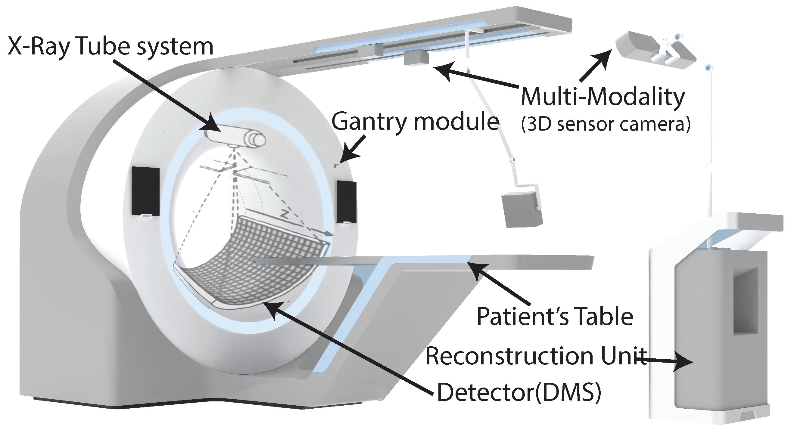
As shown in Figure 1, the CT scanner consists of an X-ray tube or source, a gantry module, a detector system (DMS), collimators, a motorized patient’s table, and an image reconstruction unit. For controlling and synchronizing all these components, different FPGAs are used in the CT scanner [18]. The X-ray tube system, collimators, and detector are fixed on the rotating disk, mounted on the gantry; the rest of the components are fixed on the stationary side. The communication between the rotating and stationary sides is done through slip-ring technology consisting of brushes that permit the electrical connection between the rotating and stationary sides.

The CT scanner works by moving the patient table to the space inside the gantry module, and when the patient’s body goes through it, the X-ray tube system and the DMS rotates around the object’s body with a frequency of about 170 rpm [16]. In the meantime, the X-ray tube system shoots a narrow beam of photons through the object’s body. The attenuated beam photons of the object’s body are acquired by detector sensors on the opposite side of the X-ray tube system [16]. The data are acquired as pixels of 2D images, called projections. Usually, modern CT scanners collect over 1160 projections per round [18]. These data are transferred to the image reconstruction unit, where the volume of the object’s body is reconstructed as volume.

The image formation in CT involves pre-processing acquired detector data, reconstructing the volume from the processed projections, and post-processing the reconstructed volume. CT reconstruction from the processed projections (total attenuation values or line integrals) is an inverse problem [19]; it means that input values (3D volumes) are estimated from the output values (2D images). Numerous solutions can be found for this problem in the literature, including the filtered back-projection (FBP) and iterative reconstruction [20,21,22,23]. Our article focuses on the X-ray pre-processing step to compute the total attenuation values from the digitized detector data. In interventional CT, it has to be executed in real time.

2.2. Pre-Processing: X-ray I0-Correction

During CT data acquisition, the patient body is irradiated with the photons emanating from the X-ray source. Some of the photons are attenuated during the photon–matter interaction. An X-ray detector detects the unattenuated or transmitted photons generating projection images. X-ray detection involves the two-level conversion process, where the X-ray photons are converted to light, and the photo-diode array converts them to electrical signals. Analog-to-digital converters (ADCs) of the acquisition system will transform electric signals into digital signals and store them in a compressed format. These 2D images are called detector data projections and are denoted by $d\left(u,v\right)$, where u and v are the detector row and column indices. Conventionally, the detector data projections are transformed into X-ray intensity projections as per the following equation:

$$I(u,v)=c·e^{-d\left(u,v\right)}$$

(1)

where c is a scaling factor. $I\left(u,v\right)$ is the intensity image data. The exponential decay of the X-ray intensity during X-ray transmission through the patient body is given by the Beer–Lambert law [20,23]. The total attenuation values along the X-ray path are given by

$$P\left(u,v\right)=ln\left(\frac{I_0\left(u,v\right)}{I\left(u,v\right)}\right)$$

(2)

where $I_0$ projections are stored in the CT system during the calibration of the scanner by acquiring the intensity projections without any object. Formula (2) is also called I0-correction. A CT 3D volume is reconstructed from the attenuation projections using state-of-the-art reconstruction algorithms.

From the detector, the DAS collects the raw sensor data which must be multiplied with a factor of f to obtain the detector data projections, as given by

$$d\left(u,v\right)=f·Raw\left(u,v\right)$$

(3)

Commercial CTs usually do not provide the projections as detector data projections, but they convert them to intensity image data. In fact, pre-processing algorithms usually process projections in intensity image data and then apply the I0-correction for the reconstruction step.

In Section 4, we propose a mathematical optimization of the I0-correction that uses directly the raw sensor data, instead of using the converted intensity image data.

2.3. Real Number Representations

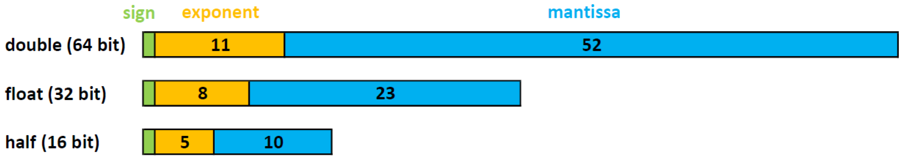
As mentioned above, the CT reconstruction algorithms use real numbers. In computing, real numbers are usually represented by the float or the double format. These formats are two different encodings of the standard for floating-point arithmetic (IEEE 754) [8]. This standard specifies conversions and arithmetic representations, and methods for binary and decimal floating-point arithmetic. As shown in Figure 2, the floating-point numbers are represented by their sign (S), exponent (E), and mantissa (M) bits. The floating-point value can be represented as a function of S, E and M, as follows:

$$f(S,E,M)=\left\{\begin{array}{lll}{(-)}^S·2^{E+1-2^{e-1}}·(1+M·2^{-m})& \mathrm{for} 0<E<2^{e-1}& \hfill \mathrm{(4)}\\ {(-)}^S·(1+M·2^{-m})& \mathrm{else}& \hfill \mathrm{(5)}\end{array}\right.$$

In the formula above, m represents the amount of mantissa bits (e.g., in single precision, floating-point m is equal to 23).

According to IEEE 754 standard, there are four different formats of encoding for the floating-point, with 16, 32, 64 and 128 bits, and they are called half-precision, single-precision, double-precision and quad-precision respectively. E and M have different data widths, based on the selected encoding, as shown in Figure 2.

The various encodings determine number representations with different accuracy. In addition, they use different arithmetic processing units, which have different performance in terms of power consumption, execution time, memory utilization, and chip area. For example, the single-precision floating point represents numbers in the range between $2^{-149}$ and $2^{128}$, with a relative error of $2^{-23}$, caused by truncating digits.

As the target data to process are limited in a small range of values, and the accuracy of the IEEE 754 representation is not required for the target application, new custom and approximate representations have been proposed in literature, with the aim to optimize hardware resources, data resources, and execution time. A proposed solution in the literature is the fixed-point representation  [24].

As shown in Figure 3, this representation is composed of three parts: sign (S), integer (I) and fraction (F) fields. There is no fixed encoding for this representation, but the hardware designer sets the size of the data width (W), that is equal to S + I + F. The size of I and F depends on the values to represent, and the desired accuracy. Furthermore, math co-processors for fixed-point operations are usually faster than the respective for the IEEE-754 standard, because the same operation implemented in fixed-point precision use fewer logic gates and hardware resources than floating-point precision, but usually it has a lower accuracy and can represent a smaller range of numbers. In Section 7, we explore different settings of the parameters S, I and F for finding the optimal configuration of these parameters with an acceptable accuracy of the CT dataset.

3. Related Works

In the literature, there are a lot of algorithms and hardware accelerators for CT pre-processing and reconstruction. Most of them use FPGAs [25,26,27,28,29,30,31], and GPUs [32,33,34,35,36] as a target platform because these offer a high level of flexibility and parallelism. Here, we do not compare the different architectures for FPGAs with the proposed CT pre-processed core because it is not possible to compare them and it is also out of the scope of our article. Instead, we are interested in optimizing the pre-processing step and investigating the impact of data formats on the reconstructed image; we only consider the different data formats used in these works. In addition, we report the related works, where the authors analyzed and compared different data formats in CT reconstruction, and point out the difference with our work that aim to find the best data format in interventional CT.

Dandekar et al. in [4] presented a reconfigurable architecture for the real-time pre-processing of interventional CT. They proposed a streaming architecture that optimizes latency. They implemented a median filtering and anisotropic diffusion filtering based on neighborhood voxels (3D pixels). This property was used for implementing a custom brick-caching schema that improves the memory performance. They describe their architecture in VHDL with different fixed-data formats: 8, 12 and 16 bits. With the custom implementation of these optimizations, they achieve a processing rate of 46 frames per second for images of size $256\times 256\times 64$ voxels.

Another important work comes from Korcyl et al. in [37]. They built real-time tomographic data processing on FPGA SoC devices. They designed the whole system from detector’s scanner to the reconstruction unit. The reconstruction system is implemented on a single FPGA board that processes the image in real-time. The architecture is composed of 8 parallel pipelines that acquire data from the scan. Inside, they de-couple the data, process them and display the images to the doctor, without using any external memory access. These FPGA accelerators for real-time CT pre-processing and reconstruction have different architectures, which use custom and standard data formats. Even if they optimize the architectures with a custom data format, they do not investigate the impact of the data format on the pre-processed and reconstructed image. They select a data format which fulfills the hardware requirements of their specific solution. In our work, we investigate the impact of the data formats on the pre-processed and reconstructed image. In addition, the CT pre-processing core can be configured at the synthesis time for using different data formats for raw sensor data, pre-processing data and reconstructed data.

For the best of our knowledge, in the literature, only Clemens Maaß et al. in [14] investigated the impact of data formats on the reconstructed image. They worked with different encodings of the IEEE-754 standard and they showed that the half-precision floating-point can enable a fast image reconstruction process without declining image quality [14]. So, instead of 32-bit single precision, 16-bit half precision is used as data format, and it reduces the traffic on the memory bus [14]. Due to arithmetic complexity, the back-projection needs to access the external memory multiple times [14]. By choosing the half-representation data format, they can reduce the data traffic and can increase the throughput of the memory bus. This work focuses on the difference between half- and single-precision floating point representation, but does not consider fixed-point representation and custom data representation, which also are used in CT image processing.

For example, Nourazar and Goossens [12] proposed an iterative CT reconstruction algorithm optimized for tensor cores of NVidia GPUs. To enhance the performance, they performed the reconstruction algorithm with a mixed-precision computation; the error of the mixed-precision computation was almost equal to single-precision (32-bit) floating-point computation [12]. Using a mixed-precision computation means that different data formats are used in the reconstruction algorithm for representing the same real value.

In our work, through a DSE, we systematically search in the design space the best data format for interventional CT. Different from Clemens Maaß et al. [14], we use a DSE in our methodology and we do not only consider the image error as the MSE and noise, but we also consider hardware cost metrics and image quality metrics, such as low contrast and uniformity. In addition, we do not limit our study to the floating-point representation, but we also consider fixed-point representation. Furthermore, with the proposed CT pre-processing core, custom data formats can be investigated.

4. X-ray I0-Correction Optimization

In this section, we describe the proposed method and formulas for performing the I0-correction directly on the acquired raw sensor data, without converting them to intensity domain images.

As explained in Section 2.2, most of the commercial CT scanners provide the projections, directly converted in the intensity domain, as real or integer number values, and the total attenuation correction is applied with Formula (2). This formula is computationally complex to implement because the logarithm operation usually is not a primitive operation in the math co-processors. In addition, for using this formula, the collected data must be converted from raw sensor data to intensity data inside the CT scanner; the conversion determines an additional latency between the DMS and the reconstruction system. In fact, for converting data from raw sensor data to intensity data, Formulas (1) and (3) are used. Formula (1) comprises an exponential operation, which is also not a primitive operation in most of math co-processors.

In our proposed optimization, we consider raw sensor data as input for the I0-correction. In this way, we have merged Formulas (1)–(3) which are usually separated and implemented in the CT data acquisition system and the reconstruction system. By merging them, we obtain the following formula:

$$P(u,v)={log}_e\left({\displaystyle \frac{c·exp(-(f·Ra{w}_0(u,v)))}{c·exp(-(f·Raw(u,v)\left)\right)}}\right)$$

(6)

If we implement Formula (6) as is, the logarithm and the power operations should be implemented. However, since we implement it inside the data acquisition system of the CT, we apply the mathematical simplification that results in the equivalent formula, shown in (7).

$$P(u,v)={log}_{10}\left(2\right)·f·(Ra{w}_0(u,v)-Raw(u,v))$$

(7)

Therefore, as shown in Formula (7), the I0-correction can be performed directly on raw sensor data with basic operations provided by most of the math co-processors. This mathematical optimization determines the decreasing of the resource utilization and execution time, compared to the implementation of Formula (6).

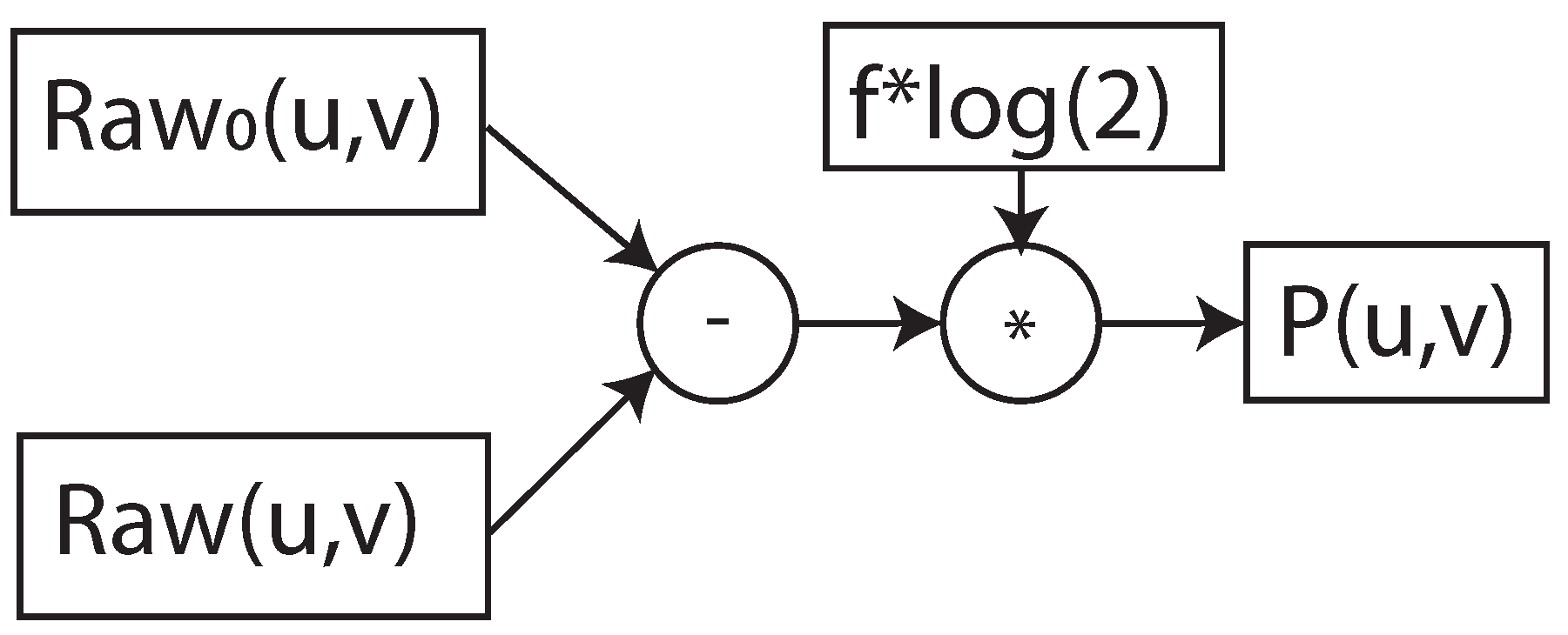
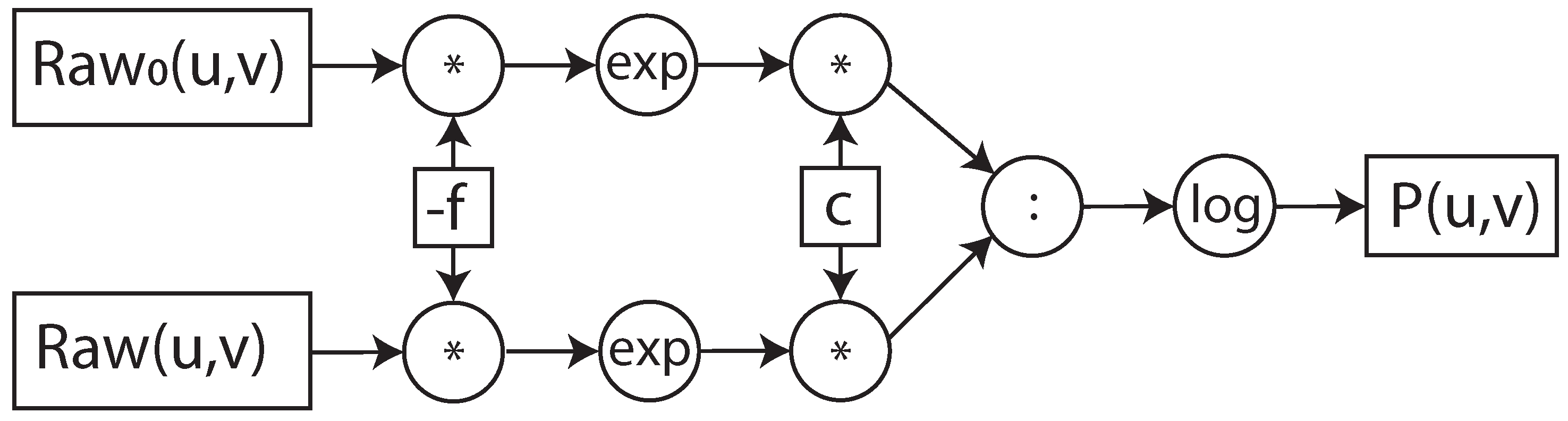
Furthermore, to perform the I0-correction and the whole pre-processing step on the fly, we propose the implementation of the algorithm in a dataflow architecture. To describe how Formulas (6) and (7) were implemented in the dataflow architecture, we used the data flow graph representation [38], as shown in Figure 4 and Figure 5. In the data flow graph the square boxes represent the input/output data and constants, the circular boxes, the operation and the arrows the flow of data. The dataflow graph shows the flow and the data and dependency of the operations. The various operations in the boxes have different latency and hardware costs in a math co-processor. The values of these metrics depend on the implemented operation and the selected data format. In the next sections, we focus on the hardware implementation of the dataflow architecture, its integration in the data acquisition system of the open-interface CT and how different data formats influence performance.

5. CT Pre-Processing Core Architecture

In this section, we describe our CT pre-processing core, which implements the I0-correction. For fulfilling the real-time requirements, the CT pre-processing core is designed as a dataflow architecture, which has a constant delay and throughput. Furthermore, to process data with high clock frequency and to reduce the critical path of the arithmetic operations, the dataflow architecture is pipelined. The depth of the pipeline depends on the data format and prepossessing algorithm, as explained in Section 9.

The CT pre-processing core, as shown in Figure 6, has the following three main stages:

• Sensor-data conversion stage: This stage obtains the pixel raw sensor data of the I0-image and the current image collected by the data acquisition system (DAS). In this stage, each pixel is converted to the selected pre-processing data format. At synthesis time, a custom configuration for floating-point or fixed-point representation must be selected.
• Image-processing stage: In this stage, pixel data are ready to be pre-processed in the selected data representation. This stage has multiple internal stages, and it is scalable for additional pre-processing steps. In this article, we focus on the pre-processing step, based on Formulas (6) and (7).
• Reconstruction conversion stage: This stage obtains the pre-processed data (attenuation image) and converts them in the reconstruction data format, defined at the synthesis time. The output results are ready for the reconstruction, and they are forwarded to the data stream unit, which is responsible either for storing or sending them to the reconstruction system.

For communicating, the CT pre-processing core uses the AXI4-Stream interface. This flexible interface can be configured with different data widths, so it can be easily used for different data representations, and integrated in any system that uses the AXI4-Stream standard.

The CT pre-processing core is designed for processing one pixel per clock cycle. If the DAS collects multiple pixels per clock cycle, multiple instances of this core must be added; in this way, all the collected pixels are processed in parallel. For example, in the integration with the DAS of our open-interface CT, we have four instances because the DAS collects four pixels per clock cycle, as is explained in the following Section 6.

Furthermore, the CT processing core is designed and implemented to be configurable for custom data representations that are defined at synthesis time. In this way, the architecture can be easily used for DSE, as it is explained in Section 7.

6. CT Pre-Processing Core Implementation and Integration

In this section, we describe the implementation of the CT pre-processing core and its integration in the DAS of a running open-interface CT. This DAS component is implemented by a ZC706 evaluation board with the XC7Z045 MPSoC-FPGA model from Xilinx [39]. An MPSoC-FPGA is a system on chip (SoC) containing an FPGA part and a processing system (PS) part with multiple CPUs and a GPU.

6.1. IP Block Design

For implementing the CT pre-processing core on the Xilinx board, we used Vitis™ HLS, which is the Xilinx high-level synthesis tool that allows C, C++, and OpenCL™ functions to become hardwired onto the device logic fabric and RAM/DSP blocks. The HSL implementation results in a register transfer level (RTL) block design, also called IP block design, which can be implemented on FPGA. Moreover, by describing our hardware components with Vitis™ HLS, we do not have to describe the arithmetic hardware components at the logic gate level. In fact, Vitis™ HLS utilizes optimized arithmetic hardware components, provided by Xilinx as a library.

The CT pre-processing core is described with C++ source code. Each stage of the dataflow architecture is encapsulated in a C++ function. The arguments of each function describe the input/output ports of the stage. In synthesis, to obtain the pipelined dataflow architecture, we use the directives “#pragma HLS DATAFLOW” and “#pragma HLS PIPELINE dataflow” provided by Vitis™ HLS. These directives allow to implement C++ loops and C++ functions as a pipelined dataflow RTL block design.

Externally, the CT pre-processing core communicates via AXI4-STREAM interfaces. These are defined by using the data format “hls::axis” and the directive “#pragma HLS INTERFACE axis”, which can be only used for the external interfaces of the core. As a result, for interconnecting the three internal stages of the CT pre-processing with a stream interface, the “hls::stream” template type and the directive “#pragma HLS STREAM variable=data format” are used.

Furthermore, we define three primitive data formats, which allow to parameterize the core for different data formats in the three main stages of the CT pre-processing core:

• Detector format: This format refers to the raw-sensor data that are generated by the DMS and collected by the data-flow module in the DAS. It defines the input data format of the sensor-data conversion stage.
• Image-processing format: This format refers to the desired data format for the pre-processing steps. It defines the output data format of the sensor-data conversion stage, the data format for the image-processing stage, and the input data format of the reconstruction conversion stage.
• Reconstruction format: This format refers to the reconstruction representation. It defines the output data format of the reconstruction conversion stage.

The designer in Vitis™ HLS defines the primitive data formats as the C++ class at synthesis time.

For DSE purposes, we configure the CT processing core with different encoding of the floating-point and fixed-point representations. For implementing these representations with the Xilinx arithmetic processing units, we use the provided libraries hls_math, hls_half, and ap_fixed. These allow us to use double, float, single, half and ap_fixed<W,I> formats. In fixed format, W refers to the data width and I the integer part of the real value number. In Section 9, the implementation results of the different configurations used in the DSE are discussed.

6.2. Open-Interface CT

Before describing the integration of the CT pre-processing core within the DAS, we introduce our open-interface CT architecture, as well as the DAS architecture, which is the central control unit of the system, the flow of data from the DMS to the reconstruction system.

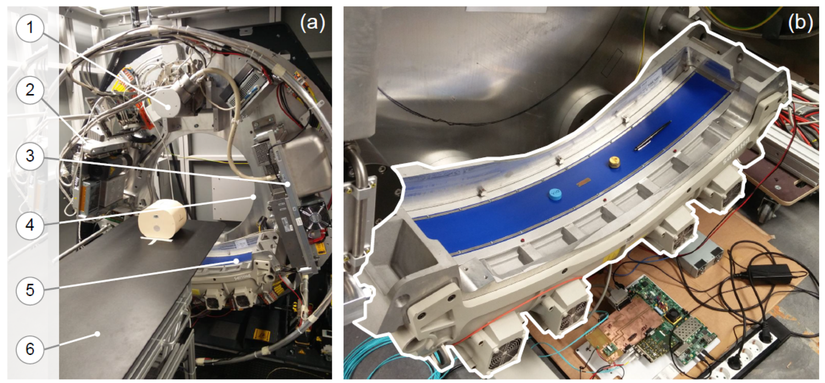
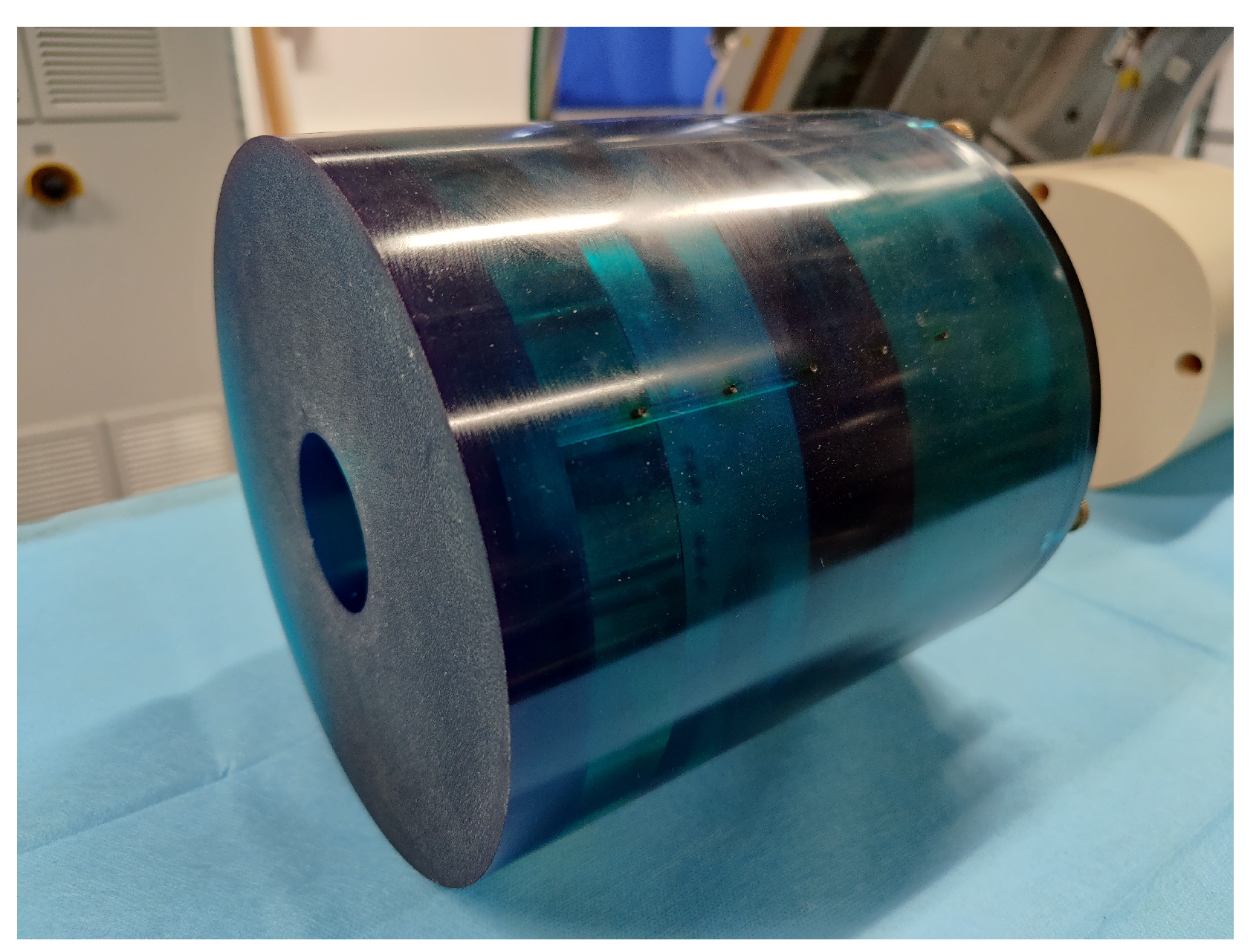
Our open-interface CT, as shown in Figure 7, consists of the following components: a 64 row DMS and an X-ray tube system, a gantry module from Schleifring [40], a patient table, and a reconstruction system. As shown in Figure 8, all these components are controlled by the DAS, which is fixed in the rotating side and is implemented on the XC7Z045 MPSoC-FPGA.

From the hardware designer prospective, the design of the open-interface CT is based on the system architecture shown in Figure 8, where the the DAS and the reconstruction systems are the components responsible for controlling and reconstructing tasks, respectively. The DAS has three main modules on the FPGA part of the MPSoC-FPGA and has a software stack on the PS part for controlling them [41].

The DAS system has the following modules, which are implemented in the FPGA part and controlled by the PS part:

• Control-synchronization module: This module is responsible for controlling and synchronizing all the external components on the stationary and the rotating sides. It is scalable, allowing an easy integration of other components in the open-interface CT, such as additional DMSs, X-ray tube systems and other sensors for multi-modality CT.
• Data-flow module: This module is responsible for collecting projections from the DMS, to manage eventually transmitting errors and to forward them to the image pre-processing module. After the pre-processing steps, it sends all the pre-processed data to the reconstruction system. It is implemented with a pipelined datapath that collects and forwards data in real time, without buffering them in external memory [42].
• Image pre-processing module: This module represents the proposed CT pre-processing core.

During the acquisition, the DMS acquires the raw sensor data and forwards them to the DAS over the gigabit interface. The raw sensor data are collected in the data-flow module of the DAS, which properly merges them and forwards to the image pre-processing module, where our CT pre-processing core is implemented. Here, the raw sensor data are converted to the selected pre-processing data format, pre-processed from raw sensor data to attenuation data and converted to the selected reconstruction data format. After that, the pre-processed attenuation data are forwarded to the reconstruction system, through the data flow module, over the gigabit slip ring connection. In the reconstruction system, the 3D volume is reconstructed.

6.3. Data Acquisition System Integration

The CT pre-processing core is integrated in the image pre-processing module of the DAS. We created the IP block design by Vitis™ HLS, and it was instantiated in the DAS design as the IP core by using Vivado Design Suite.

Based on the DAS, the DMS and the reconstruction algorithm requirements, we set the clock frequency, the input and output data representations of our CT processing core, as follows:

• clock frequency = 100 MHz: It is the clock frequency for collecting data.
• input data = short format: It is a 16-bit unsigned representation, which is used for the raw sensor data.
• output data = float format: It is a 32-bit single-precision floating-point representation, which is used for the reconstruction algorithm.

Due to these requirements, we set these two data formats in the sensor-data conversion stage and the reconstruction conversion stage, respectively. Yet, in the image-processing stage, we explored different data formats, with the aim to find the optimal data format for interventional CT application.

7. Design Space Exploration

In this section, we explain our approach for the design space exploration of the different data formats and representations, applied on the pre-processing step. In addition, we describe the parameters and the metrics used to find the optimal data format and representation.

The DSE of all possible data representations in CT applications is time consuming. In fact, for each input configuration, the 3D volume must be reconstructed, and the image quality analysis must be performed. Due to that, it results in a complex problem, where it is impossible to analyze all configurations for the different representations in the design space. To simplify the exploration process, we define two steps that limit the size of the problem itself. First, we make the “pre-selection of data formats and representations” for the input parameters, and after that the “pre-selection of metrics”. In this way, we reduce the set of input parameters and decrease the evaluation time of each solution. As input parameter, we also have the clock frequency, but it does not affect the image quality, so we set it at 100 MHz. The value of the set frequency is based on the data-rate of the collected data. In this way, we decrease the design space because different clock frequencies can generate different design performances in resource utilization and latency.

7.1. Pre-Selection of Data Formats and Representations

To pre-select the data formats and reduce the size of the design space, we use a top–down approach. At the beginning, we decided to explore only standardized data formats that are also implemented in the new commercial architectures, such as GPUs, and TPUs. In this way, we focused on floating-point and fixed-point representations.

For interventional CT applications, the goal is to minimize latency while maintaining high accuracy for having a real-time reconstruction. For this reason, in the second step, from the pre-selected data representations, we considered only formats with data widths in the range from 16 to 32. The values of this range are related to the data widths of raw sensor data and reconstructed data. In fact, raw sensor data are usually represented with short format (16-bit data width), and reconstructed data with float format (16-bit data width). In addition, we considered the double format (64-bit data width), which we used as a reference point in the image quality analysis. Therefore, for the floating-point representation, we limited our study to three different encodings: half, single and double precision.

By contrast, regarding the fixed-point representation with a fixed-rounding configuration, if all possible formats in the range from 16 to 32 bits are considered, 408 configuration formats are possible. Therefore, we considered only the upper bound and lower bound configurations, which are 16 and 32 bits. For these two data widths, there are 16 plus 32 possible configurations as fixed-point representation. Therefore, to reduce our DSE from these 48 to the desired 2 configurations, we analyzed the raw sensor data and selected one configuration for 32-bit fixed-point and one for 16 bit fixed point. The raw sensor data are represented as 16-bit unsigned, so we configured the 32-bit fixed-point with I and F both equal to 16 bits. In this way, the 32-bit fixed-point does not approximate any values in the sensor data conversion stage.

Due to the fractional part of the fixed-point representation, the 16-bit fixed point cannot contain the 16-bit unsigned, without approximation. Therefore, to find the best configuration, we started from the 16-bit fixed-point configuration that has 8 bits for integer and fractional, and we estimated the MSE. The MSE is the mean squared difference between a reference value and an approximated value [43]. This is often used to measure the image quality between two images [44]. To find other configurations, we analyzed the multiplication factor of Formula (7), which can be approximated with a shift of the dot in the number. So, we removed the multiplication and shifted the dot by decreasing/increasing the integer and fractional parts, respectively, to reach the lowest MSE. In this way, we reached the best configuration of 16-bit fixed-point with 4-bit and 12-bit for the integer and fraction parts, respectively.

With this methodology, we pre-selected four data representations for the DSE, which are half-precision and single-precision floating-point, and 16-bit and 32-bit fixed point, where I and F are equal to 16 and 16 bits, and equal to 4 and 12 bits, respectively.

7.2. Selection of Metrics

To reduce the time involved in the DSE for generating the different results, we also selected metrics that are significant for the hardware performance and the image quality analysis in the case of interventional CT.

For the hardware performance evaluation, we considered the resource utilization of the FPGA and the execution time of the different solutions. In our case, we only analyzed the execution time of the CT pre-processing core, which is expressed as latency from the Vitis™ HLS tool. For analyzing the resource utilization of the FPGA, we considered the configurable blocks and memories mostly used for image processing applications. These are digital signal processing (DSP) blocks, flip-flop registers (FF), BRAM memory, and look-up tables (LUTs) for the combinatorial logic [45].

For the image quality analysis, of the different solutions, we considered the following metrics: MSE of the 2D projections, and noise, low contrast and uniformity of the reconstructed 3D volume. The MSE was applied on the 2D projections for measuring if the collected data have an acceptable accuracy for the reconstruction. In this way, we only reconstructed and performed the image quality analysis on acceptable configurations. The other selected metrics for the image quality analysis are useful for interventional CT applications. The uniformity and noise metrics are important to identify the eventual image degradation, caused by the arithmetic approximation of the different data formats. The low contrast metric is important for tumor detection [15], useful in tumor ablation, during surgery.

8. Image Quality Analysis

For performing the image quality analysis, we considered three elements: the CT acquisition configuration, the significant metrics, and a representative phantom. Usually, most of the work in the literature considers different CT scanners and/or acquisition configurations to research how these elements influence the image quality [46,47,48]. However, in our research, we are interested in comprehending the influence of the data formats on the image quality, independently by the CT scanner and acquisition configuration. Therefore for our experiments, we used one scanner with a single configuration for the CT acquisition. Additionally, we used the CATPHAN^® 500 [15], which is a representative phantom. In fact, this provides the complete characterization for maximizing the image quality.

8.1. CATPHAN^® 500

The CATPHAN^® 500 [15], as shown in Figure 9, has four modules enclosed in a 20 cm housing. Each module is used for performing different image quality metrics, such as geometry alignment, uniformity, noise and low contrast. Before describing the modules, we introduce the Hounsfield unit (HU), also referred as the “CT number”. It is the relative quantitative measurement of radio density [49]. Radiologists uses it in the interpretation of CT images because different body tissues have different densities.

We scanned the different modules with the same CT scanner configuration. Based on the pre-selected metrics, we used the three following modules:

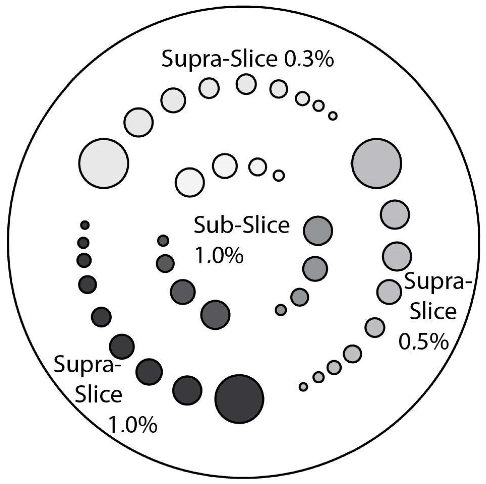
• CTP515 Low Contrast Module: This module consists of a series of cylindrical rods of various diameters and three contrast levels to measure low contrast performance [15]. The roads, as shown in Figure 10, are provided on z-axis positions, for avoiding any volume-averaging errors [50]. The different low contrast are useful for identifying small low contrast objects, such as tumors. Subslice targets have a nominal 1.0% contrast and z-axis lengths of 3, 5, and 7 mm. For each of these lengths, there are targets with diameters of 3, 5, 7 and 9 mm [50]. We acquired this phantom section to perform the low contrast image quality for the different data formats.
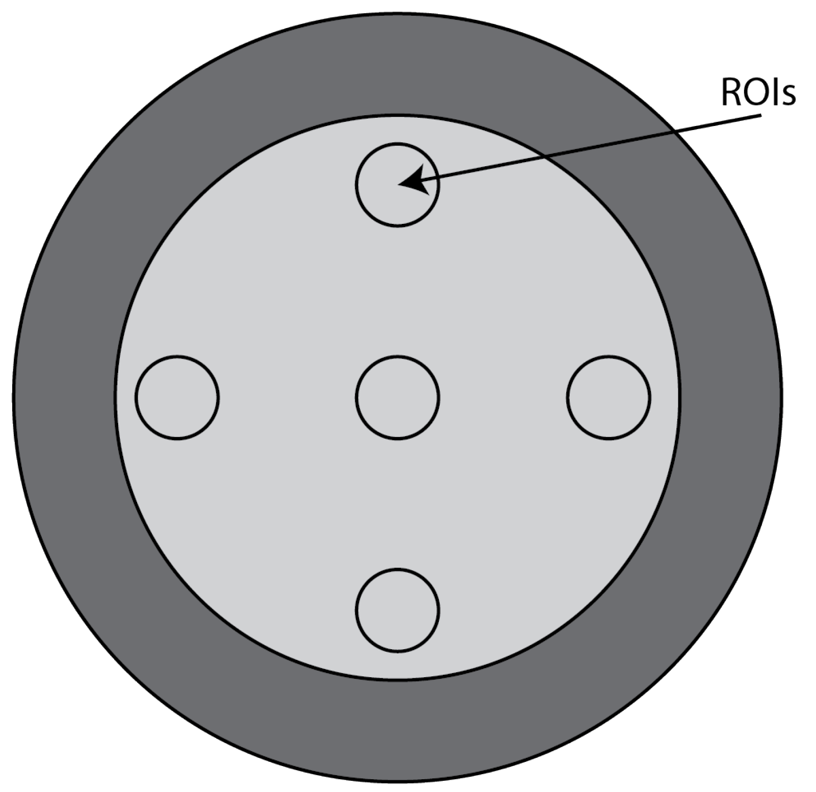
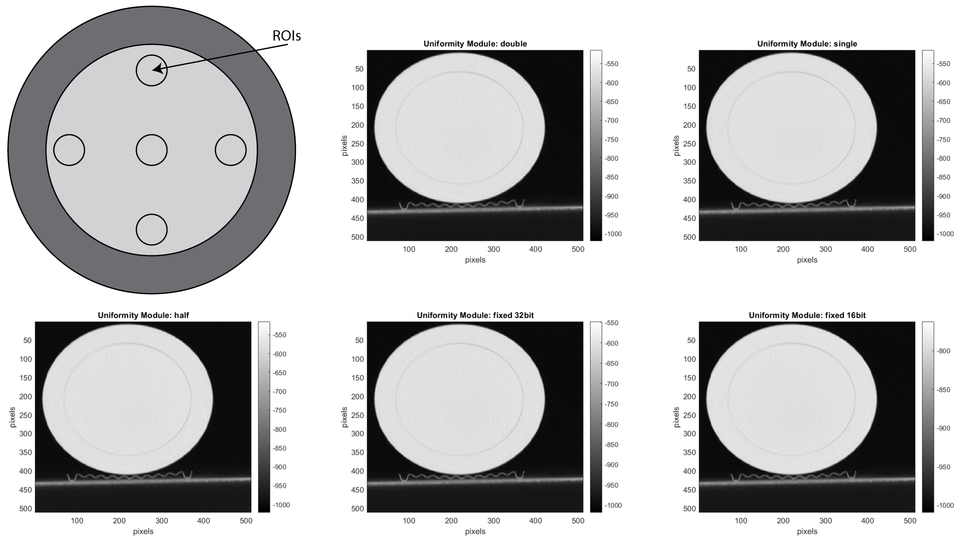
• CTP486 Uniformity Module: This module is cast from a uniform material with a “CT number” designed to be within 2% of water’s density under standard scanning protocols [15]. This module is used for measurements of spatial uniformity, which means CT number and noise value. As shown in Figure 11, this module has a different region of interest (ROI) that can be targeted for measuring the uniformity of the different areas of a phantom section. In fact, the mean CT number and standard deviation of a large number of points, in a given ROI of the scan, is determined for central and peripheral locations within the scan image for each format of the scanning protocol [50].
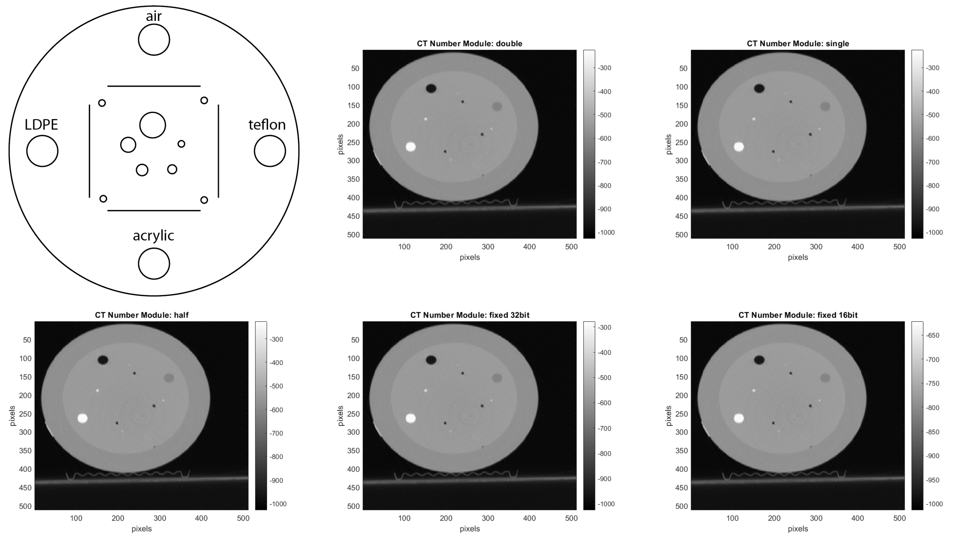
• CTP401 Slice Geometry and Sensitometry Module: This module is used to verify the phantom position. The module, as shown in Figure 12, includes four sensitometry targets (Teflon, Acrylic, LDPE and Air) to measure the CT number linearity [15]. The module also contains five acrylic spheres to evaluate the scanner’s imaging of subslice spherical volumes. The diameters of the acrylic spheres are 2 mm, 4 mm, 6 mm, 8 mm, and 10 mm. We used this phantom for a human visual analysis of the CT images, in relation to the different materials and the size of the spheres.

8.2. CT Acquisition Configuration

In the open-interface CT, we manually set-up the components with the following parameters:

• X-ray tube system

  –

  Voltage: 120 KV

  –

  Intensity: 250 mA

• Detector system

  –

  Number of row slices: 64

  –

  x and y slice width: 0.625 mm

  –

  Number of projections per round: 1160

  –

  Size of the projection matrix in pixel: 672 × 64

• Gantry system

  –

  Number of rounds per second: 1

• Reconstruction system

  –

  Reconstruction algorithm: Feldkamp (FDK) algorithm [21]

  –

  z slice width: 1 mm

  –

  Size of the reconstructed matrix in pixel: 512 × 512

Furthermore, we pre-acquired and stored the I0-images, which are the projections without phantom of one round. Figure 13 shows one of these projections stored as a short data format.

Since, the I0-images are in the original raw sensor data, we only acquired it once, when we started our experiments.

8.3. Image Quality Metrics Calculation

For each image quality parameter, we used a mathematical estimation of it. For the pixel error of the 2D projections, we calculated the MSE, which gives the error interpretation of the approximated image [44]. The formula of MSE is the following:

$$MSE=\frac{1}{V}\sum _{j=1}^V{\left(A_j-S_j\right)}^2$$

(8)

Here, $A_j$ is the pixel value of the main image and $S_j$ is the pixel value of the estimated image [43]. As the main image, we selected the pre-processed image with double format.

For calculating the values of the noise, uniformity and low contrast from the reconstructed volume, we considered a different ROI per module, as suggested by the CATPHAN^® 500 Manual [15]. For selecting the ROI, we used the reconstructed images shown with red and blue circles in Figure 14, where the pre-processing was done with the double format. For the noise analysis, we calculated the standard deviation of the CT number for each of the ROIs, placed on the uniformity module and shown in Figure 14.

For the uniformity analysis, five ROIs with 40 pixels in diameter are placed on the module, four peripheral ROIs and one central ROI. The average CT number, in HU, is obtained for each of these ROIs, and the uniformity is measured as the maximum difference between the mean value of the center ROI and one of the peripheral ROIs.

For the low contrast analysis, we calculated the contrast noise ratio (CNR) by placing a ROI of 20 pixels in diameter in the larger targets of both the supra-slice 1.0% and supra-slice 0.5%, and in the background area right beside it. The CNR was calculated using Formula (9) and averaged over 32 reconstructed slices.

$$CNR=\frac{\left|S_T-S_B\right|}{{\sigma }_B}$$

(9)

In Formula (9), $S_A$ and $S_B$ are the signal intensity of the supra-slice target and the background region, respectively, and ${\sigma }_B$ is the standard deviation of the background.

9. Results and Discussion

This section shows and discusses the results of the proposed optimized method with the different data formats used in the DSE. First, we compare the proposed method and the standard method presented in Section 2.2. Second, we compare and discuss the results of the pre-processing step and reconstruction image for the different data format configurations selected within the DSE. Finally, we define which data format seems to be the best for the pre-processing step in interventional CT.

We used Vitis™ HLS for the hardware performance analysis in terms of hardware cost. In this article, we focus on the resource utilization and execution time of the CT pre-processing core, which is configured to process one pixel per clock cycle. If the DAS collects multiple pixels per clock cycle, multiple instances of the CT pre-processing core must be added to the design. Due to the data parallelism, the resource utilization increases linearly, while the overall execution time remains constant. In the reported results, we selected the XC7Z045 MPSoC-FPGA model from Xilinx [39] as the FPGA target platform.

9.1. Standard and Optimized Methods

As explained in Section 4, the standard method for I0-correction and the optimized method were implemented in the CT pre-processing core. The two versions, shown in Figure 4 and Figure 5, were implemented with pipelining. In the optimized version, the logarithm operation is pre-calculated because its argument is constant. The algorithm executes only subtraction and multiplication operations. By contrast, the standard method executes an additional power operation and logarithm operations, which are expensive in terms of execution time and resource utilization. To compare and quantify the two methods independently by the data format, we selected the same image-processing format (single-precision floating point), and synthesized both with Vitis™ HLS. Furthermore, we analyzed the MSE of the 2D pre-processed projections. The estimated MSE is $3.21\times {10}^{-15}$, which is almost 0. With the reported low MSE, we also validated our solution and we can confirm that the two methods are equivalent, as expected from the mathematical simplification. In fact, both methods generate the same output projections. The MSE is not exactly 0 because the two methods evolve different operations and math co-processors components that approximate the values in different ways.

As expected, the two methods differ in terms of hardware performance. The optimized method, as reported in

Table 1. Hardware report for CT pre-processing core (instance for 1 pixel per clock cycle).

Precision Name	BRAM 18K	DSP	FF	LUT	Latency
Standard method (float)	2	30	3497	6881	660 ns
Optimized method (float)	0	5	527	785	160 ns

, does not use any BRAM and requires about 10 times less DSP, FF and LUT resources, the standard method to perform a complex operation, as logarithm and power need to buffer data; for this reason, BRAM is utilized. In addition, these complex operations determine the higher LUT, FF and DSP utilization. FPGAs have a small limited number of DSPs, and therefore, their utilization should be minimized, when it is possible. Moreover, the low required resource utilization for our solution allows to implement and integrate the pre-processing core directly in the DMS, closest to the sensor.

Due to the real-time requirements, the most important metric is the execution time/latency. In this case, we analyzed the latency of the single operations for the two methods; the results are also shown in Table 1. The standard method has a latency of 660 ns, while the optimized method has a latency of 160 ns. In the standard method, there are power, division and logarithm operations that are much slower operations than subtraction and multiplication operations. In fact, the optimized method has only one multiplication and one subtraction, which have low latency, as shown in

Table 2. Timing analysis of the standard method.

1st Stage		2nd Stage						3rd Stage
Buffer	Conv.	Mul.	Exp.	Div.	Div.	Log.	Muls	Buffer
10 ns	50 ns	40 ns	140 ns	120 ns	120 ns	130 ns	40 ns	10 ns

and discussed in Section 9.2. For this reason, our solution achieves a speed-up of about 4.125× compared to the standard method with the same data format. We see that in the optimized method configured with the 32 bit-fixed point data format, we reach a speed-up of about 16.5× compared to the standard method. This latency enhancement is a significant improvement for the real-time requirements of the interventional CT application.

By using the dataflow architecture, both solutions make it possible to pre-process a new pixel each clock cycle. It was not possible to compare the optimized methods with the related works, in terms of hardware implementation, due to the lack of information. Related works provide the whole execution time, without considering the pre-processing step and its impact on reconstruction.

9.2. Comparison of the Data Formats

Before analyzing the results of the different data format configurations with the pre-selected metrics, we performed a human visual analysis of the CTP401 module. In the human visual analysis, we observed that the pre-processing step was well performed and the grid between sensors was removed. Figure 15 shows the 2D projections pre- and post-processing with the different data format configurations. Yet, we did not observe differences between the different configurations with the human visual analysis.

The human visual analysis was conducted also for the reconstructed images, shown in Figure 16. We observed that all target materials can be distinguished independently by the data format configuration utilized in the pre-processing step. This means that the image quality does not seem to change in terms of human visual analysis.

Since with the human visual analysis, it is not possible to compare the accuracy and the information lost between the different data formats, we estimated the MSE of the projections. The MSE, as explained in Section 7, is the key point used for reducing the eligible data formats for the DSE. It was crucial to select the two data format configurations of the 16-bit and 32-bit fixed-point; we reduced from 48 to 2 possible data format configurations. The MSE is a reasonable metric in this step because it can be applied to 2D projections before the reconstruction. In addition, we noticed that it is in the same order of magnitude for the different phantoms. However, the MSE does not consider all image quality metrics, which are significant to understanding how data formats influence the quality of reconstructed images. Therefore, we performed the measurement of low contrast, noise and uniformity for the reconstructed images. For calculating these metrics, we acquired, pre-processed with different data format configurations, and reconstructed the modules shown in Figure 17 and Figure 18.

The results of the image quality analysis are shown in

Table 3. Image quality estimation of different data format configurations.

Resource Name	Half	Float	Double	Fixed 16	Fixed 32
MSE	2.39 × 10${}^{-7}$	3.21 × 10${}^{-15}$	0	0.22	0.0039
CNR Supra-Slice 1.0% [$\Delta$HU]	0.555	0.566	0.566	0.335	0.536
Noise [HU]	5.8	5.7	5.7	2.7	5.3
Uniformity [$\Delta$HU]	3.54	3.57	3.57	2.44	3.5

. We observed that the MSE of all configurations is lower than 1. This value is very good in terms of image quality since the MSE is usually between 2.36 and 2.37 also in medical image compression [51]. By comparing the other image quality metrics of all data formats with the double format, the values were judged to be good in most of the cases. In fact, these are in the same order of magnitude as shown in Table 3. The only data format where the approximation of the pre-processing has slightly influenced the reconstructed images is the 16-bit fixed point. Due to the approximation made and the bit truncation involved for converting the raw sensor data from 16-bit unsigned to 16-bit fixed point, the low contrast pixels are blurred. Therefore, the contrast noise ratio (CNR) is about 0.2 lower than the double configuration. By contrast, due to the blurred low contrast pixels of the 16-bit fixed-point configuration, a lower noise and a better uniformity was estimated for this configuration, compared to other data formats. In fact, in images with blurred pixels, the pixel values are similar, and therefore, there is a lower noise and a better uniformity. From this image quality analysis, we can conclude that all data formats result in an acceptable pre-processed and reconstructed image quality. The 16-bit fixed point has some problems that would make sense to choose it only if the hardware cost has much advantages, compared to other solutions.

To define the hardware costs of the different data types, we compared the resource utilization and the latency of the various data format configurations. As shown in

Table 4. Resource utilization of different data format configurations.

Resource Name	Half	Float	Double	Fixed 16	Fixed 32
BRAM 18k	0	0	0	0	0
DSP	4	5	14	1	0
FF	382	527	1292	167	309
LUT	223	785	1796	941	1245

, the utilization of all FPGA resources decreases from floating-point to fixed-point representations, independently of the data width. In fact, DSPs are minimized from 14 of the double configurations to 0 and 1 of the 32-bit fixed-point and 16-bit fixed-point configurations, respectively. In FPGA, the number of DSPs is crucial because they are in the order of hundreds, while LUTs and FFs are in the order of hundreds of thousands. Therefore, the low utilization of resources in fixed-point representations allows the FPGA to implement additional pre-processing steps on the fly. The best result comes from the 32-bit fixed point; this configuration is the only one that utilizes 0 DSPs and implements all operations with LUTs and FFs. Therefore, even if it utilizes more LUTs than 16-bit fixed-point, we can confirm that 32-bit fixed-point is the data format with the best performance in terms of resource utilization concerning the FPGA available resources. The 32-bit fixed-point has better performance than the 16-bit fixed-point due to the fact that Vitis™ HLS optimizes the 32-bit fixed-point format in the provided libraries.

Finally, we analyzed the execution time in the different cases. The results in

Table 5. Timing analysis of different data format configurations; all values are expressed in $ns$.

		1st Stage		2nd Stage			3rd Stage
Configuration	Total	Read	Conv.	Buffer	Sub.	Mul.	Conv.	Write
Half	190	10	50	20	50	40	10	10
Float	160	10	50	0	50	40	0	10
Double	220	10	50	0	70	60	20	10
Fixed 16-bit	70	0	0	0	10	30	20	10
Fixed 32-bit	40	0	0	0	10	10	10	10

show the advantage of using fixed-point representation compared to floating-point representation. In fact, 16-bit and 32-bit fixed-point configurations are 2.2× and 4× faster than the single-precision floating-point configuration, respectively. The conversion between the collected data and fixed-point representation is faster than floating-point representation because it is implemented with a combinatorial shift, which is implemented in hardware with a bitwise assignment. Due to that, the conversion is implemented together with the subtraction, which is also implemented with combinatorial logic. For this reason, the reported conversion execution time is close to 0.

As mentioned above, due to the Vitis™ HLS optimization and the DSP optimization, 32-bit fixed-point configuration implements all operations with FFs and LUTs; therefore, it has also lower latency than 16-bit fixed-point configuration. In fact, the former configuration does not use DSPs for the multiplication, so its execution time is 10 ns (1 clock cycles). By contrast, as shown in Table 5, due to the DSPs latency, the latter configuration spent 30 ns (3 clock cycles) for the multiplication, which is the time required by DSP to process one operation.

To compare all the metrics of various configurations, we used the radar graphs shown in Figure 19. Since the values have different units and scales, the min-max normalization is used [52]. Double configuration has the maximum quality and hardware performance, so it has most of the values equal to 1. By analyzing and comparing all results, we found that the 32-bit fixed-point configuration is optimal for interventional CT pre-processing in terms of image quality and resource utilization.

The 32-bit fixed point is the best compromise between image quality and hardware preference. It maximizes the hardware performance, and the image quality after the reconstruction decreases only 7% in comparison with the double format. In contrast to [14], we do not consider the required external memory bandwidth for the different configurations because we are interested in finding only the best data format configuration in the pre-processing step. In this step, our CT pre-processing core processes projections on the fly and does not use any external memory, which usually is the main bottleneck GPU and CPU solutions.

10. Summary

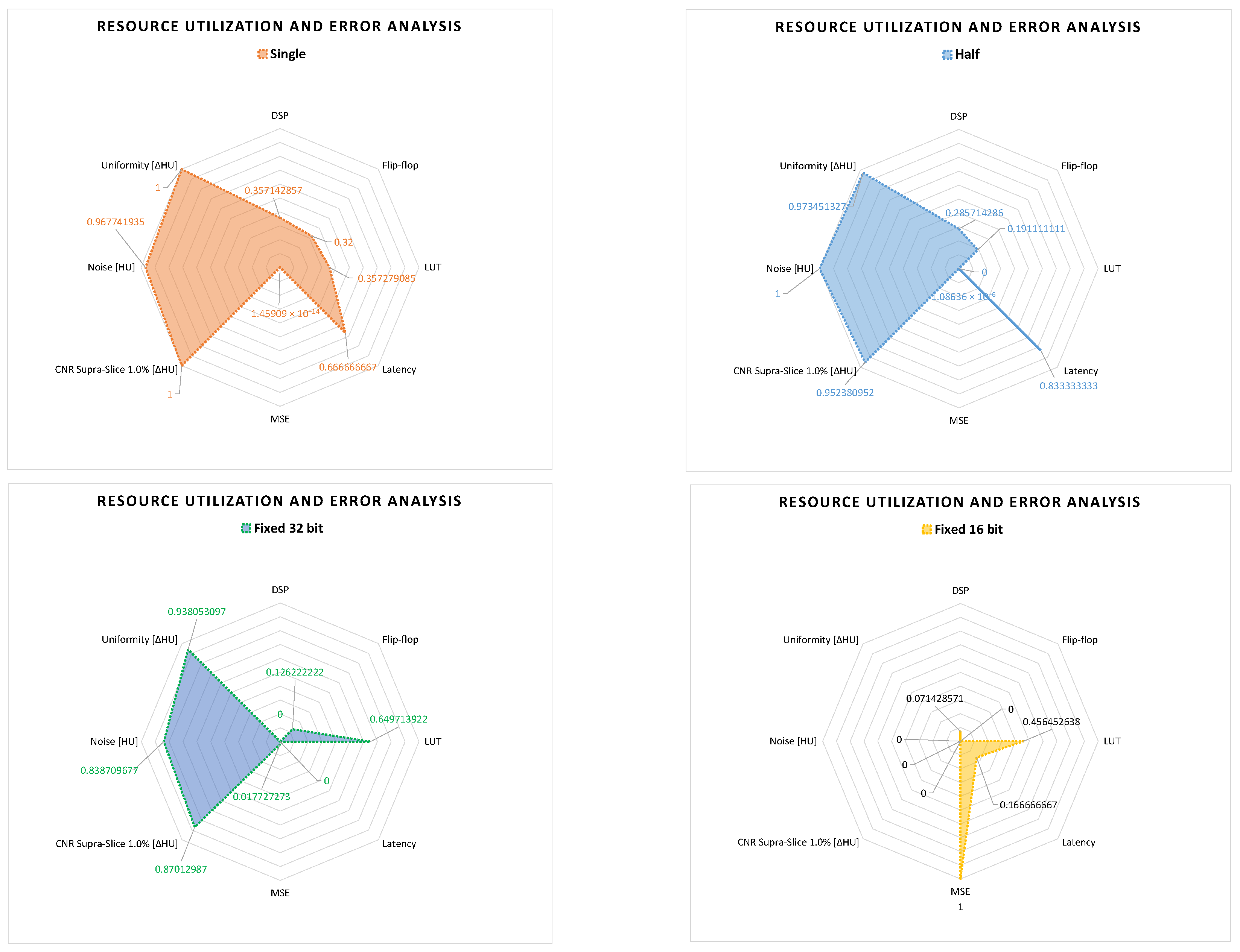
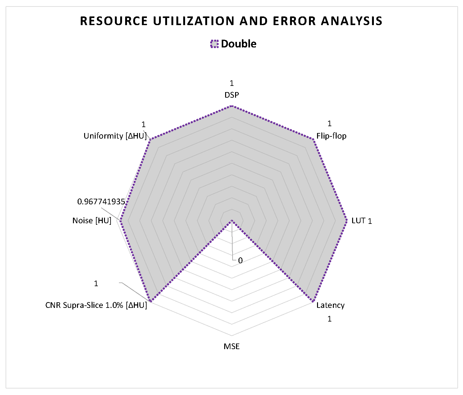
In this article, we proposed a hardware acceleration of the pre-processing step for interventional CT. By performing this algorithm on the raw sensor data, we reduced the number of operations and their complexity. In addition, with this optimization, we achieved a speed-up of about 4.125× compared to the standard method. Furthermore, we have implemented the algorithm in the proposed CT pre-processing core. This FPGA accelerator pre-processes CT projections on the fly and can be configured for pre-processing pixels with different data formats. In addition, we performed a design space exploration of the different data formats between double, float, half floating point, and the different configurations of 16-bit and 32-bit fixed point. Among them, we found out that 32-bit fixed point is the optimal data format for pre-processing steps in interventional CT. In fact, with 32-bit fixed point, we achieve a speed-up of 16.5× compared to the standard method, and it utilizes less FPGA resources. Additionally, with 32-bit fixed point, the image quality of the reconstructed image decreases only about 7% compared to the double format. In future works, we aim to extend this exploration also to the reconstruction step, where mixed-precision data formats could be used.