Research Status of and Trends in 3D Geological Property Modeling Methods: A Review

Abstract

Three-dimensional (3D) geological property modeling is used to quantitatively characterize various geological attributes in 3D space based on geostatistics with the help of computer visualization technology, and the results are often stored in grid data. The 3D geological property modeling includes two main components, grid model generation and property interpolation. In this review article, the existing grid generation methods are systematically investigated, and both traditional and multiple-point geostatistical algorithms involved in interpolation methods are comprehensively analyzed. It is shown that considering the numerical simulation of oil reservoirs, the orthogonal hexahedral grid remains the most suitable grid model for simulations in petroleum exploration and development. For the interpolation methods aspect, most geological phenomena are nonstationary, to simulate various types of reservoirs; the main development trends are increasing geological constraints and reducing the limitation of stationarity. Both methods have certain constraints, and the multiscale problem of multiple-point geostatistics poses a main challenge to the field. In addition, the deep-learning based method is a new trend in geological property modeling.

1. Introduction

Three-dimensional (3D) geological property modeling refers to the quantitative characterization of various geological features in 3D space in digital form based on geostatistics using computer visualization technology. It serves as the basis for evaluating mineral resource assessments, reservoir physical property simulations, and reservoir numerical simulations [1,2]. To better understand the 3D geological property modeling, the systematic analysis and review of the current research are needed.

The main application of 3D property modeling in the petroleum field is to establish a geological model of the reservoir; this type of modeling is therefore also called reservoir modeling. The characterization of 3D reservoir models provides an in-depth understanding of the macroscopic distribution, internal structure, physical parameters, and variation characteristics of oil and gas reservoirs, and this understanding is of great importance for oil and gas exploration and development [3]. Geostatistics, which is the core method of 3D property modeling, was proposed by Journel in the 1970s for application in petroleum exploration and development [4,5] and has been widely used and developed since then. The advantage of geostatistics is its ability to integrate data according to the source and reliability of the data and to integrate various information, such as core, log, and seismic data, into the model while ensuring data consistency. In addition, geostatistics can also provide uncertainty assessment as a basis for risk evaluation. In China, research on the theory, methods, and applications of geostatistics started around the 1980s [6], and the application of geostatistics in reservoir descriptions for reservoir geological modeling began in the early 1990s. Since Qiu [7] introduced the related work on reservoir modeling, Zhang and Wang [8], Yu and Li [9], and Zhang et al. [10] successively carried out research on reservoir modeling methods for actual reservoirs in China; this research laid the foundation for applying reservoir modeling technology in oilfield development. Since then, with the development of computer technology and the research of numerous studies in petroleum science and technology, the methods and techniques of reservoir modeling and its application to various reservoir types have developed rapidly.

The oil and gas reservoirs in China are mainly terrestrial oil reservoirs with very complex subsurface conditions; consequently, establishing a 3D property model for reservoir characterization is difficult. At present, most oilfields have entered the middle and late stages of development and are in a state of high water content. The balance between injection and production poses an increasingly prominent problem, so it is especially important to determine the amount and distribution of the remaining oil in the reservoir. In addition, today’s petroleum exploration and development focus on unconventional oil and gas reservoirs, such as shale gas and tight sandstone gas. Although such oil and gas reservoirs are abundant in China, they are characterized by low porosity, low permeability, and high water saturation. Therefore, compared with that of conventional oil and gas reservoirs, the development of unconventional oil and gas reservoirs is bound to pose new requirements for reservoir modeling. To solve these problems, there is an urgent need to establish a more refined reservoir model. Therefore, it is necessary to study grid framework models and geostatistical theories and methods in depth so that they can accurately characterize the reservoir at various levels and describe the heterogeneity of the reservoir while quantitatively evaluating the uncertainty of the model and reducing the risk of exploration and development. Therefore, studying 3D property modeling methods can provide a powerful tool for improving the recovery of oil reservoirs in China and offer theoretical guidance for effectively recovering the remaining oil and developing unconventional oil and gas reservoirs.

3D property modeling represents the heterogeneity of properties in the geological body, thereby reflecting the distribution of the characteristic values of a certain class of physical and chemical properties of the geological body in 3D space, and the results are stored in raster data [11,12]. Based on this definition, 3D property modeling includes two main components: 3D grid model generation and property interpolation. In petroleum exploration and development, the 3D raster model is also referred to as the reservoir grid, and due to the complexity of the physical structure of the reservoir, geostatistics are applied to the model’s property interpolation.

In this article, 3D geological property modeling methods and their applicability are analyzed from these aforementioned two aspects. In detail, the existing grid generation methods are systematically investigated, and both traditional and multiple-point geostatistical algorithms involved in interpolation methods are comprehensively analyzed. Several conclusions are drawn from these analysis.

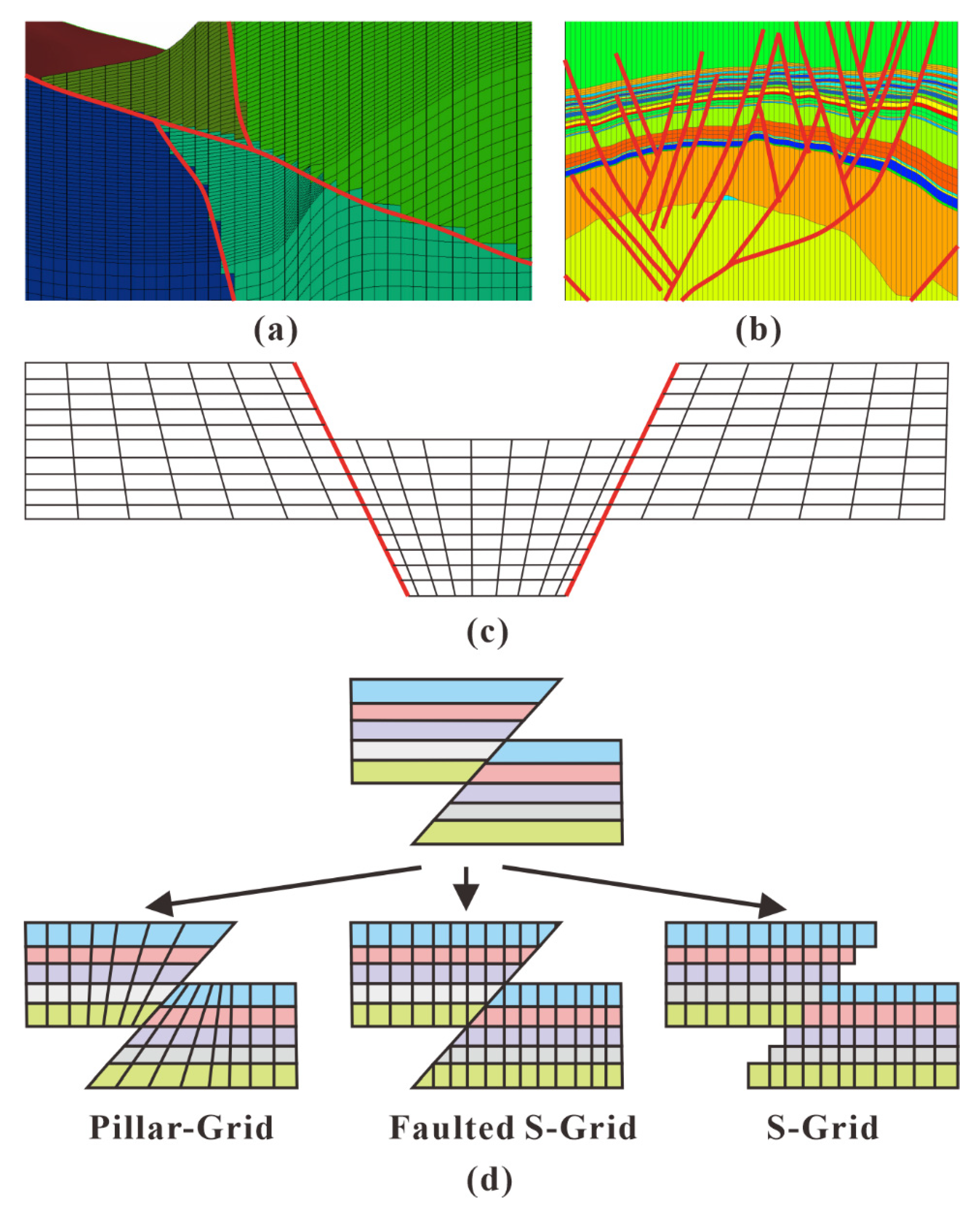
2. Research on Reservoir Grid Generation Method

Building a 3D reservoir grid model is a key intermediate process and importantly affects the subsequent reservoir property modeling and numerical simulation based on geostatistics. In modeling a reservoir by using geostatistical tools, the gridding process essentially determines how to characterize the macroscopic homogeneity of the reservoir. Since geostatistics are implemented on logical grids, a grid with excessive and excessively large distortion can easily cause the variogram to become distorted, thus affecting the accuracy and reliability of the modeling of properties, such as sedimentary facies and pore permeability [13,14]. Additionally, the shape and resolution of the grid affect the accuracy and speed of the numerical simulation of the reservoir [14,15].

Research on reservoir grid models has been carried out for many years, resulting in many grid types. Zakrevsky [16] conducted comprehensive gridding and outlined the general procedure of grid generation. Reservoir grids are categorized mainly into structured grids and unstructured grids. Structured grids are typically generated using hexahedra and are organized in an orderly manner with i, j, and k, such as Cartesian grids and corner point grids, while unstructured grids include tetrahedral grids and perpendicular bisector (PEBI) grids. In stratified deposits such as oil sand, often, the Cartesian grid is transformed to a stratigraphic grid using a non-linear coordinate transformation, which is referred to as unfolding. Thom [17] compared the characteristics of the s-grid, faulted s-grid, and pillar grid as well as these grids’ performance differences in property distribution, grid coarsening, and numerical simulation. As show in Figure 1, For the s-grid, faulted s-grid, and pillar grid, the main difference is that they contain different fault treatment approaches. Three different examples are extracted in Figure 1a–c, and the conceptual models are drawn, as show in Figure 1d, to show the different fault treatment approaches. S-grid is also known as stair-step grid; the sides of this kind of grid cell remain vertical and are controlled by an orthogonal footprint [17], as show in Figure 1a. Faulted s-grid is known as Jewel Grid; the grid cells are split exactly at the local position of the fault plane, as show in Figure 1b [17]. Pillar grid is widely used in petroleum engineering, and the most common grid is the corner point grid. For the position of faults, the pillar that controls the grid cells is parallel with the fault lines. Thus, the fault should be simplified when the fault is too complicated, as shown in Figure 1c.

Gringarten et al. and Mallet et al. [18,19] divided the grids into “geological grids” for geostatistical property modeling and “fluid simulation grids” for numerical simulation based on the different needs of reservoir modelers and digital modeling engineers for grid use. In the many grid studies, the corner point grid represented by the pillar grid has been the hotspot of research, with the most mature application. Pillar grid generation involves three main steps [20,21]: (1) a fault model is formed by simulating the fault using pillars; (2) gridding is carried out by combining fault pillars into a 3D grid framework; and (3) vertical stratification is conducted by generating initial layer surfaces on the grid framework for geological stratification. The pillar grid is characterized by its grid orientation along fault lines, boundary lines, or pinch-out lines, indicating that the grid can be distorted, thus overcoming the inflexibility of the orthogonal Cartesian grids and allowing for easy simulations of faults, boundaries, and pinch-outs [22,23]. With the development of technology and the continuous improvement in reservoir simulation accuracy, the defects of the pillar grid are gradually exposed as follows. First, due to the limitation of the geometric location of pillars, it is necessary to simplify the fault when using pillars to construct a complex fault network. Second, on the one hand, the nonorthogonality of the pillar grid makes calculating conductivity during numerical simulation difficult; on the other hand, the nonorthogonality of the pillar grid affects the accuracy of the results. Ruiu [24] proposed a grid generation method that adopts the form of a Cartesian grid at the global level and simulates the fault by truncating the hexahedron, thereby finally constructing an XY-orthogonal and locally truncated grid model. This grid can express the shape of the fault while avoiding the loss of orthogonality due to distortion, but the grid generates many polyhedral grids in models with many faults, thereby also affecting the fluid simulation operations. After analyzing the limitations of the pillar grid, Gringarten [25] proposed a vertical stair-step grid that is more suitable for fluid simulation and experimentally demonstrated that this type of grid outperforms the pillar grid in terms of grid coarsening and fluid simulation; the author did not give the method for generating this grid.

In addition, many studies have been devoted to unstructured grids. The PEBI grid is flexible and locally orthogonal, thus reducing the influence of grid orientation on the results. In 1988, Heinemann et al. [26] proposed the implementation of the PEBI grid based on the Voronoi diagram for the numerical simulation of the reservoir grid and then improved the grid with dynamic refinement as needed [27,28,29]. Palagi of Stanford University [30,31,32] studied the use of the Voronoi grid, which is essentially the PEBI grid, to simulate vertical and horizontal wells and performed numerical simulation of reservoirs. Since then, scholars have successively carried out research on 3D PEBI grids along with investigation and improvement in different application environments [33,34,35,36]. Additionally, many studies on PEBI grids have been published in recent years by Chinese researchers. Xie [37] and Lin et al. [38,39,40] systematically elaborated the application of PEBI grids in the numerical simulation of reservoirs. Liu [41] addressed the problem of fine numerical simulation of reservoirs by adopting an idea of a hybrid grid consisting of a radial grid in the oil well area and a PEBI grid in the reservoir area. Ref. [42] proposed a similar idea on hybrid grids.

Xiang [43] and Zha [44,45,46] studied the generation algorithm of two-dimensional (2D) PEBI grids, but did not fully address the generation algorithm of 3D PEBI grids. In general, the numerical simulation solutions of PEBI grids are not mature enough and not widely used. In addition, the research on PEBI grids is mainly for the numerical simulation of reservoirs; there are few studies on how PEBI grids are generated and maintain geological significance in geological modeling. In other words, other grids generally need to be transformed before PEBI grids can be used for the numerical simulation of reservoirs.

3. Interpolation Methods for 3D Property Modeling

3.1. Traditional Geostatistical Methods

There is often much spatial variability when dealing with subsurface space modeling in Earth science. Proposed by Matheron [47], geostatistics is a tool to quantify this variability to enable geologists to predict behavior and make the most useful decisions under the constraints of limited knowledge and resources. The major techniques for generating a 3D model of the geological variables are the main focus, especially the interpolation methods; thus, the principal component analysis (PCA), maximum autocorrelation factor (MAF), projection pursuit multivariate transform (PPMT), and related methods are not considered. The PCA, MAF, PPMT, and other multivariate transforms methods are commonly used to simulate correlated variables independently without the requirement of fitting a linear model. In addition, these approaches can be applied in the data preparation procedure for the geostatistics approaches dealing with multivariate analysis.

Geological phenomena, especially in the petroleum industry, follow a series of complex physical rules that cannot be expressed by simplified models. Reservoir properties, such as porosity and permeability, are needed in reservoir fluid simulation equations to predict oil production and are required at each spatial location; however, porosity and permeability can be obtained only in sparse wells. In other words, for economic reasons, it is generally impossible to accurately and definitively obtain all the information required for a subsurface model. Therefore, spatial uncertainty is a fundamental concept in Earth science. In the early days of the oil industry, practitioners tended to think deterministically and thus expected to obtain a single estimate of oil production. Today, uncertainty is widely accepted.

Geostatistics captures this spatial uncertainty by generating multiple reasonable property models (also known as stochastic realization). By integrating information from different sources, such as logging, coring, geological interpretation, or seismic data, the study area and the true expression of this uncertainty can be obtained. Matheron [48] introduced the regionalized variable $Z\left(h\right)$ as the value of characteristic $Z$ of a geological phenomenon at location u. Regionalization means that variables expand in space and exhibit a specific spatial structure. If this concept is ignored, the variables are randomly distributed in the reference region and thus do not exhibit any spatial continuity. However, physical processes in geology are not random in space and have spatial continuity in their properties. For example, the continuity of the river channel formed by a river flowing down the hillside is controlled by the complex physical phenomena along the path of the river, and the mineral deposits tend to be concentrated in certain specific spaces. Thus, the regionalization of variables is the main principle by which geostatistics differs from statistics. It would be impossible to make predictions if spatial continuity does not exist. However, the physical laws that determine spatial continuity cannot be accurately modeled due to the lack of information. To quantify spatial uncertainty, a mathematical model is needed to describe the spatial structure of the variables in the study area. For example, the spatial trends in the data and the isotropy or anisotropy of the variables can be obtained by defining a spatial variable model in geostatistics.

Geostatistical methods have evolved over the decades into two-point geostatistical methods (including the kriging method, deterministic simulation method, and stochastic simulation methods), object-based methods, and multiple-point geostatistics. The methods differ in how their spatial continuity and uncertainty models are expressed and how direct data (such as core data) or indirect data (such as seismic data) are integrated for stochastic realization of subsurface conditions. These methods are described in the following sections, with an emphasis on multiple-point geostatistics as a focus in this article.

3.1.1. Kriging Method

The kriging method was proposed by Krige [49] in 1951 for estimating unknown variables. The method uses the linear least-squares estimation technique and relies on variables from sparse and valid hard data for interpolation. This method was initially applied to mineral deposits under the assumption of continuity of measured mineral grades using a variogram. As show in Figure 2, the variogram has several main components: range, nugget, arch height, and sill.

The range refers to the range where regionalized variables have spatial correlation. Within the variable range, the data are correlated, while outside the variable range, the data are not correlated with each other; the observed values outside the variable range will not affect the estimation results.

If the variation function is discontinuous at the origin, this is called the nugget effect in geostatistics, which shows that it has large spatial variability in a very short distance. The spatial variability is the nugget. It should be noted that it can be caused by geological variability or measurement error.

The arch height refers to the difference between the sill and the nugget.

Sill is the total spatial variability of the whole variables. When the value of the variation function at distance is greater than the range, the sum of the nugget value and arch height is the sill.

The kriging method uses linear combinations of known data to obtain values at unsampled locations without assuming any statistical distribution. The weights for these linear combinations need to be calculated to minimize the estimated variance in a least-squares sense, which can be expressed by the following least-squares variance equation:

$${\lambda }_a={\left[z\left(u\right)-z^{*}\left(u\right)\right]}^2$$

(1)

where ${\lambda }_a$ represents the value of the linear combination weight and $z^{*}$ represents the estimated value of the random variable $z$ at location $u$; the linear estimate of $z^{*}$ is obtained as follows:

$$z^{*}\left(u\right)-m\left(u\right)={\displaystyle \sum _{\alpha =1}^n{\lambda }_{\alpha }}\cdot \left[z\left(u_{\alpha }\right)-m\left(u_{\alpha }\right)\right]$$

(2)

where $m$ denotes the mean at the unsampled location u and ${\lambda }_{\alpha }\left(\alpha =1,2,\dots ,n\right)$ denotes the weight of n measured variables.

In two-point geostatistics, the structural function that characterizes the spatial variability of a variable is called the variogram, which is the spatial correlation between any two points in the space. That is, as the distance between two points in the space increases, the variogram gives the change in the spatial correlation between them. This is the simplest way to correlate the value of an unsampled point with its neighboring observations. Under stationary conditions, the variogram is defined in probability theory as follows:

$$2\gamma \left(h\right)=E\left\{{\left[z\left(u\right)-z\left(u+h\right)\right]}^2\right\}$$

(3)

where $\gamma \left(h\right)$ denotes the variogram value calculated based on the pairing of the available data for a particular lag distance; $E$ denotes the expected squared error of the estimation point, $z$ denotes the random variable, and $h$ denotes the relative distance from location $u$.

The kriging method can describe only relatively simple geological features, and the simple variogram fails to apply to some geological phenomena with high variability. To address this problem, many scholars have conducted research and improvements. Depending on the interpolation model and application environment, a variety of kriging methods (e.g., simple kriging and ordinary kriging) have emerged [5,50,51]. The kriging method is characterized by underestimating high values and overestimating low values, limiting its ability to simulate nonlinear spatial structures. However, in some cases, what is important is not the estimated value of the variable itself but the variable’s nonlinear function, such as estimating the mineral grade greater than a certain threshold. Indicator kriging [52] was proposed to simulate this nonlinear geological model. In addition, multivariate geostatistics was introduced for the problem of correlations between multiple variables. Cokriging [53,54] is a method for linearly estimating one variable from several other variables. For example, the value of porosity can be estimated from a linear combination of the measured values of nearby porosity and the corresponding acoustic impedance values. The applicability, advantages, and disadvantages of common Kriging methods are shown in

Table 1. Comparison of different Kriging Methods.

Kriging Method	Applicability		Advantages	Disadvantages
Simple Kriging	Satisfy the second-order stationary condition; It is suitable for the situation with small spatial variability; The expectation of the random function at each position point is a known constant		The algorithm is simple, fast and widely used	The second-order stationary condition cannot be satisfied in practice; Cannot be used in situations with any trend; Need to know the expectation of variables
Ordinary Kriging	Satisfy the second-order stationary condition; It is suitable for the situation with large spatial variability; The random function of each position point should have expectation; The expectation of random function at each position can be different; The data distribution shall not have obvious trend		There is no need to predict expectations; The algorithm is simple, fast and widely used	The second-order stationary condition cannot be satisfied in practice; It cannot be used in situations with obvious trends
Universal Kriging	Satisfy the second-order stationary condition; It is suitable for the situation with large spatial variability; The random function of each position point should have expectation; The expectation of random function at each position can be different; The data distribution shall not have obvious trend The attribute does not satisfy the general stationary assumption; Showing a trend in a certain direction; After filtering out the drift of the original data, ensure that the residual is stable		The algorithm is simple and fast; For geological conditions with obvious trend, the interpolation result is better than simple and ordinary Kriging	The selection of mathematical function form representing drift has a certain error; The residual interpolation variogram needs to be estimated; For complex data distribution, the drift part is difficult to obtain
External Drift Kriging	External variables need to reflect the spatial distribution trend of main variables; The distribution of external variables in space is known and changes smoothly		Compared with the interpolation method based on logging data, the result obtained by external information participating in interpolation is more accurate	When the external variables are not smooth, the stability of the algorithm is poor
Collocated Co-kriging	At the position of the estimation point, the secondary variable must be known	The parameters shall meet the second-order stability; It is applicable to the case where there are few observed data of the estimated variable	Only the secondary variables with the same position as the estimated variables need to be retained, and the secondary variables of all data points are not required; Collaborative simulation, interpolation results are more accurate; Secondary variables have little effect on the accuracy of estimation	When the study area is large and there are few reliable data, the reliability of the interpolation results is not good
Intrinsic Collocated Co-kriging	The secondary data are retained at location being estimated and at the primary data locations

.

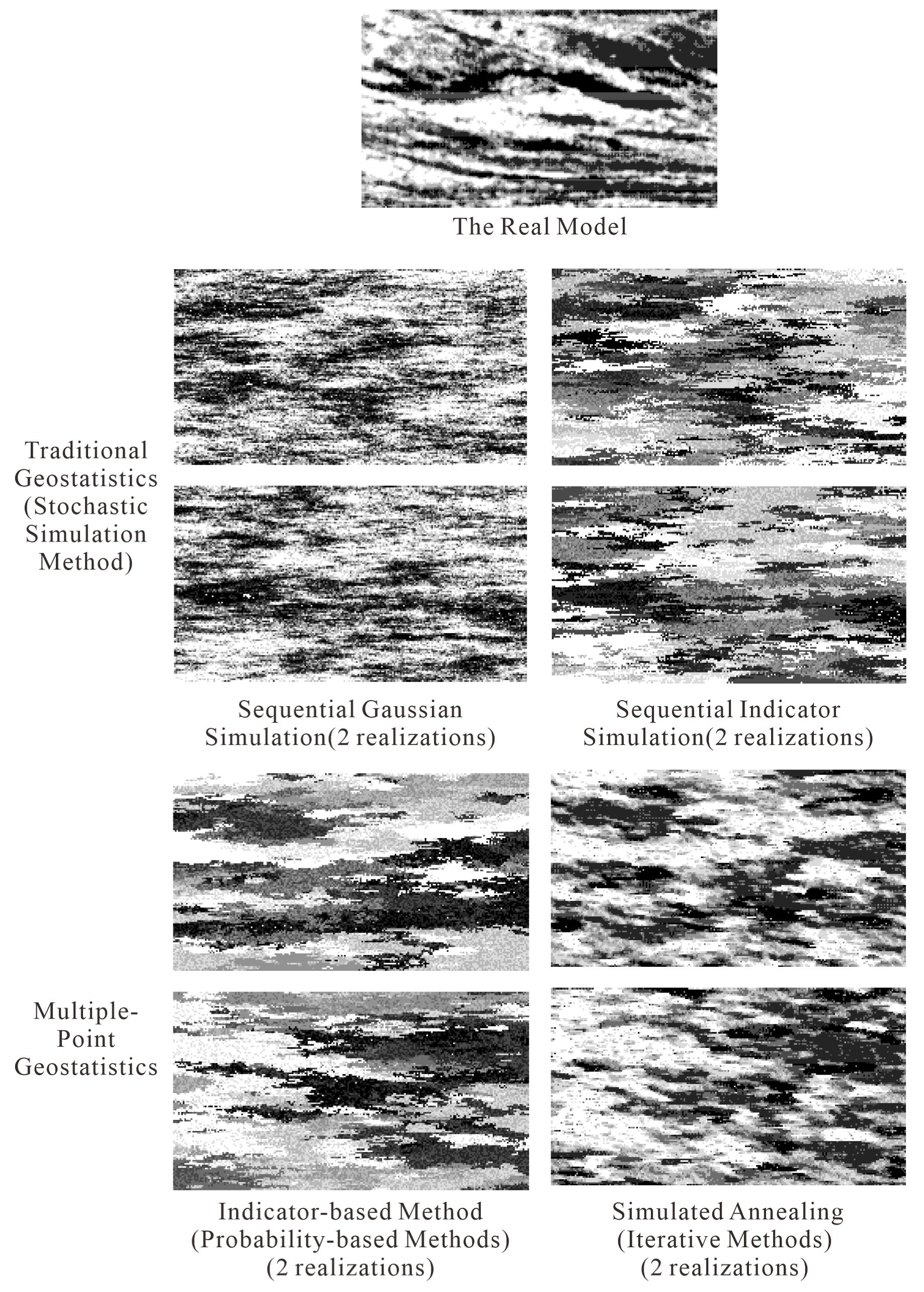
3.1.2. Stochastic Simulation Method

All kriging methods derive the “optimal linear unbiased estimator” based on variogram models. Therefore, kriging methods are only a smooth representation of the subsurface model. Due to uncertainties, it is not enough to generate a single deterministic model. Therefore, optional stochastic reservoir modeling methods are needed to establish a series of models with different property distributions.

Stochastic simulation was first introduced by Matheron [55] and Journel [4] to correct the smoothing effect and other human factors in the kriging method. Stochastic simulation also uses the variation model to predict the spatial variability, resulting in multiple optional models of the spatial distribution of variables in the study area. The main differences between the kriging method and the stochastic simulation method [48] are that the kriging method performs the “optimal” linear estimation of the variables without conducting statistical analysis of the estimated values together; that is, the results of the kriging method are a local presentation of the variables, while the stochastic simulation method provides a global expression of the variables, which can reproduce the spatial continuity pattern.

The stochastic simulation process is also called sequential simulation and is particularly important for numerical simulations of, for example, the control of fluid flow in a reservoir by permeability. Therefore, global stochastic simulation algorithms outperform the locally accurate kriging methods in constructing reservoir models. The smoothing effect of the kriging method introduces significant bias when dealing with nonlinear problems. In addition to providing a variety of optional results, sequential simulation can also truly characterize the spatial variability of geological phenomena. Multiple conclusions about reservoir connectivity or fluid mobility can be summarized from the results of each realization. Therefore, functions that characterize complex nonlinear structures can be obtained by calculating each simulation result and then obtaining the probability distribution of the target variables.

Stochastic simulation is based on a simple mathematical principle, which mainly aims to obtain the conditional probability $z$ of the variable $Z\left(u\right)$ after calculating all values at the neighboring locations of $u$. For $N$ random variables of $N$ valid data types $\left\{z_{\alpha }=z\left(u_{\alpha }\right),\alpha =1,2,\dots ,N\right\}$, the N-dimensional conditional probability distribution function is expressed as Equation (4).

$$F\left(Z_1,Z_2,\dots ,Z_N|\left(n\right)\right)=\mathrm{Prob}\left\{Z_{\alpha }<z_{\alpha },\alpha =1,2,\dots ,n|\left(n\right)\right\}$$

(4)

Using Bayes’ theorem, the N-dimensional probability distribution can be obtained by calculating the univariate conditional probability distribution function as Equation (5).

$$F\left(Z_1,Z_2,\dots ,Z_N|\left(n\right)\right)=F\left(Z_1\left(n\right)\right)\cdot F\left(Z_2\left(n+1\right)\right)\cdots F\left(Z_N\left(n+N-1\right)\right)$$

(5)

Therefore, the general process of sequential simulation is summarized as follows:

Calculate the univariate conditional probability $z_1$ of $Z_1$, conditional on $n$ original data.

Calculate the conditional probability $z_2$ of $Z_2$, conditional on $n$ original data and the previously simulated value $Z_1=z_1$.

Calculate the conditional probability of $Z_N$, conditional on $n$ original data and $N-1$ previously simulated values.

Next, the two main stochastic simulation methods, i.e., the sequential Gaussian simulation for continuous variables and sequential indicator simulation for discrete variables, are described.

Sequential Gaussian Simulation

Sequential Gaussian simulation has been widely used because of its simplicity and flexibility due to the introduction of a Gaussian assumption. Sequential Gaussian simulation has a simple basic idea: each variable is simulated according to the normal conditional probability distribution function obtained by a simple kriging method, which selects the expected value of the variable as the estimated value of the point to be estimated. Then, the expected value and variance are used to establish a Gaussian distribution, from which a value is randomly selected as the simulated value, which is generated using a random drawing from a CDF (Monte Carlo Simulation). The simulation procedure of the continuous variable $Z\left(u\right)$ is as follows:

Calculate the univariate conditional probability distribution function $F\left(z\right)$ for the study area.

Convert $Z$ to a normal distribution.

Define random paths to visit the grid nodes.

Search for known data nearby and previously simulated data.

Calculate the expected value and variance of the conditional distribution by using a simple kriging method.

Obtain an estimated value according to the conditional distribution and assign the value to the node.

Continue to the next grid node until the end of the path.

Convert the strong normal distribution back to the initial univariate conditional distribution function $F\left(z\right)$.

In this process, different results are obtained for each random path so that a variety of results that meet the requirements can be used to analyze the uncertainty.

The applicability, advantages, and disadvantages of common Sequential Gaussian Simulation methods are shown in

Table 2. Comparison of different sequential Gaussian simulation methods.

Kriging Method	Applicability	Advantages	Disadvantages
Sequential Gaussian Simulation	Random variables conform to Gaussian distribution, or conform to Gaussian distribution after data transformation; For continuous variables	With different random paths each time, different simulation effects are obtained. According to geological experience, the most suitable simulation results are selected	It is not suitable for continuous variables with strong anisotropy; The accuracy of simulation results is closely related to the variation function
Sequential Gaussian collocated collaborative simulation	Random variables conform to Gaussian distribution, or conform to Gaussian distribution after data transformation; Applicable to continuous variables; At the position of the estimation point, the spatial distribution of external variables is known; The main variable and external variable satisfy the second-order stationary	Using external parameter collaborative simulation, the interpolation result is more accurate	It is not suitable for continuous variables with strong anisotropy; The accuracy of simulation results is closely related to the variation function

.

Sequential Indicator Simulation

One problem with sequential Gaussian simulation is the simulation’s inability to express the spatial correlations between simulated extreme values [56,57]. Sequential Gaussian simulation uses a covariance model to describe the subsurface space, but in some cases, the continuity of spatial variables varies with range. For example, shales show good continuity when the permeability is lower than a certain value, but the sequential Gaussian simulation underestimates this continuity. In other words, the simulation’s estimated values at the long tail end of the probability distribution (the extreme end of the probability distribution) are spatially uncorrelated. Addressing this problem requires nonlinear sequential indicator simulation methods. The sequential indicator simulation method obtains the local probability distribution of discrete data through a certain variogram with a given threshold and then establishes discrete images [56,58]. The indicator technique can specify indicator variograms for different facies, and more importantly, this technique can integrate a variety of soft data [50,59].

In the indicator simulation, some thresholds $z_i=1,\dots ,N$ need to be set to discretize random variables. The data are either discrete (e.g., facies) or continuous. Continuous data need to be transformed into discrete variables with the threshold $z_i$ by indicator transformation (Equation (6)):

$$I\left(u;z_i\right)=\{\begin{array}{c}1,\mathrm{if} Z\left(u\right)<z_i\\ 0,\mathrm{if} Z\left(u\right)\ge z_i\end{array}$$

(6)

Then, the experimental indicator variogram can be derived as follows for each threshold (Equation (7)):

$$\gamma \left(h;z_i\right)=E\left\{{\left[I\left(u;z_i\right)-z\left(u+h;z_i\right)\right]}^2\right\}$$

(7)

The simulation process is similar to that of sequential Gaussian simulation. The nodes are first randomly visited, a conditional distribution is established, and then the estimated value of the current node is obtained from the probability distribution function. Finally, the simulation of the next node continues with the data constraints of the previously estimated nodes added until all the nodes are simulated.

3.1.3. Object-Based Method

Geostatistical interpolation algorithms include sequential simulation methods [51,52,60,61,62], iterative methods [63], and noniterative and nonsequential simulation methods [64,65]. However, these are all two-point statistical methods based on the definition of variograms and cannot simulate complex spatial patterns, such as rivers. Simulating complex spatial patterns is very important in fluid simulation. Therefore, many attempts have been made to reproduce nonlinear spatial structures. For example, the anisotropy directions of the variogram are modified at local locations, and the continuity of geological features is improved by modifying the range of the variogram [66]. However, none of these approaches can truly reproduce complex geological patterns.

The object-based method [67,68,69,70,71] distributes geometric objects by using the marked point process based on some probability theory. This method directly inputs geometric objects into the grid until certain predefined constraints are met. This process requires iterative trials and constantly editing and modifying the shape and location of the object to achieve a result conforming to the constraint information. A major advantage of the object-based method is that the model can achieve good visual effects, thereby allowing geologists to see familiar sedimentary objects and directly adjust the objects’ shape and size. For example, a river channel can be characterized by sinuosity (amplitude and wavelength), channel width, channel length, and channel thickness. Thus, by defining the aforementioned attributes using a random distribution function, several channels can be employed in the model to form meandering stream facies, as shown in Figure 3. Nevertheless, the object-based method still has some drawbacks. First, it is difficult to constrain the data faithfully, and it is quite complicated to consider dense well point data while repeatedly modifying the object position. Second, the multivariate distribution of the marked point process is also very complex and difficult to analyze and define.

3.2. Multiple-Point Geostatistics Methods

The two-point geostatistical method uses the spatial correlation between any two points in the space or uses this correlation as a simple variogram of the spatial continuity model for interpolation. This method relies only on the relationship between two points, but in practice, the correlation of multiple points at once is desired. The formation process of geological heterogeneity is very complex and cannot be expressed by a two-point variogram model. Some complex geological phenomena, such as meandering river systems, cannot be described by traditional random function models. As shown in Figure 4, there are three different spatial structures. For the variogram East–West, situation 1 and situation 2 are almost the same, while the spatial structures are totally different. Meanwhile, for the variogram North–South, the 3 spatial structures are alike. The variation function cannot fully reflect the spatial structure. Therefore, multiple-point geostatistics are introduced to simulate this highly complex geological feature [72]. The two-point geostatistical method differs from the object-based method and is more likely to be faithful to valid data.

The idea of multiple-point geostatistics is to use more than two points to infer unknown random variables. Traditional methods consider a stochastic model between two points; that is, the spatial continuity is assumed to be linear. Multiple-point geostatistics uses a structure of more than two points for statistical inference; consequently, this method can reproduce nonlinear spatial correlations. However, in practical applications, it is difficult to find enough points, especially in the case of sparse data, thus not allowing direct inference of subsurface information or the establishment of a random function model that can describe the spatial structure. Therefore, it is necessary to use the conceptual image of geometric properties and geological features (which may be built using the interpreted geological data) for multiple-point geostatistical inference. Such a conceptual image is called a training image.

The training image can be established from geological phenomena, such as the simulation of river sedimentation. The corresponding inference does not come from real data but from the simulated data depicted by the training image. In geological work, by simulating geological processes and even making outcrop photographs, one can depict waterways or lobes and can make multiple-point geostatistical inference with photographs. Since the training image covers multiple points, its spatial continuity pattern is more complex and comprehensive than that of the variogram. Therefore, the training image is closely related to the sedimentary conditions. However, it is not faithful to any specific data but is simply a conceptual image that characterizes the subsurface space. Therefore, it is appropriate to use the object-based method to generate a training image that meets the requirement.

In 1993, Guardiano [72] studied the algorithmic implementation of multiple-point geostatistics. This implementation first assumes an n-dimensional template $\left(h_1,h_2,\dots ,h_n\right)$ and then scans the training image by using the template for all n random variables $Z_1=z\left(u+h_1\right),\dots ,Z_n=z\left(u+h_n\right)$ to derive the experimental conditional distribution of $Z\left(u\right)$ at point u. Finally, a sample value $Z\left(u\right)$ is taken from this distribution and assigned to the current grid to be estimated. A sequential-like method is used here to simulate all grid points randomly. As show in Figure 5, a 2 × 2 scan frame is applied. For a target training image, the scan frame is employed to scan all the parts to obtain different data events. Different data events have different probabilities. When reconstructing the new image, the different probabilities are employed.

However, this algorithm has not been very practical due to its excessive computational complexity. With the increasing demand for modeling complex reservoirs with heterogeneous sedimentary characteristics, a variety of multiple-point geostatistical methods have been subsequently developed. These methods all perform multiple-point geostatistical inference through conceptual training images and can be classified into three categories according to their different simulation methods: (1) probability-based methods, (2) iterative methods, and (3) pattern-based methods.

3.2.1. Probability-Based Methods

Single Normal Extended Simulation (SNESIM)

Proposed by Strebelle [73,74], SNESIM is a probabilistic method similar to, and an improvement of, the one proposed by Guardiano and is used for simulating discrete variables. To reduce the computational complexity of conditional probability, SNESIM no longer scans the training image for each conditional data template; instead, SNESIM scans the training image once and stores all probabilities in a search tree. This search tree structure makes it possible to quickly obtain the required conditional probabilities during simulations. SNESIM is a pixel-based sequential simulation method and is more likely than the object-based method to be faithful to well seismic data. One of SNESIM’s drawbacks is that the training image must be unconditional and cannot be used for continuous variables. Moreover, the SNESIM algorithm can capture only the static features of the training image. In addition, any trend, such as vertical or area ratio change, needs to be defined explicitly.

Indicator-Based Method

Some researchers have attempted to combine multiple-point probabilities with indicator techniques. For example, Ortiz [75] incorporated multiple-point geostatistics by using an indicator technique under the assumption of conditional independence in the Bayesian framework and between information sources. In this technique, multiple-point statistics are obtained directly from valid data. At each location of the grid, the conditional probability derived from the multiple-point information is integrated with the conditional probability obtained by the indicator kriging technique as the property value of this location. Later, Ortiz [76] proposed another method that can integrate multiple-point geostatistics into all traditional sequential methods.

Impala

Impala is a probability-based multiple-point simulation method that uses lists. Impala follows the same principle as SNESIM in that Impala stores conditional probabilities obtained from the training image and then uses them in the simulation. The difference is that Impala uses a list structure instead of the SNESIM search tree to store the multiple-point statistics inferred from the training image [77], thereby reducing the storage capacity of the multiple-point simulation (MPS) algorithm. In addition, Impala can obtain conditional probabilities in parallel. Despite the storage and central processing unit (CPU) advantages of using lists, the implementation of this method is very similar to that of the SNESIM algorithm.

3.2.2. Iterative Methods

Simulated Annealing (SA)

SA is a global optimization method that can reduce specific objective functions. The first application of SA in space was introduced by Reference [78]. This algorithm generates a model by iteratively minimizing the objective function, which characterizes the degree of mismatch between the desired statistic and the spatial continuity of the a priori model.

The process starts by simulating a random spatial distribution of values on the grid. In each iteration, the node values on the grid are perturbed, and a new mismatch between the current statistic and the target statistic is quantified. This perturbation is retained only when the degree of mismatch is reduced, i.e., when the objective function is reduced. However, to reach the global minimum without falling into a local minimum, the SA method sometimes discards the perturbations with low mismatches or even accepts unfavorable perturbations in a so-called “annealing scheme”. The grid is updated continuously and iteratively in this process to achieve the multiple-point statistics of the training image.

This iterative method has been applied to the simulation of categorical variables [79] or the simulation of the physical properties of continuous rocks [80]. The optimization of the objective function in SA relies on the subjective selection of optimization parameters and perturbation mechanisms for efficient simulation. Many studies have attempted to select the initial temperature [81] or update the objective function and the perturbation mechanism in SA optimization [82]. However, in general, these parameters strongly depend on the spatial continuity model and need to be set through trial and error.

Later, Peredo [83] applied the SA method in parallel computing to reduce the computational cost. Despite these efforts, the simple visual effect comparison of geometric features in the implementation shows that considering only the low-order statistics of the spatial model (because of the computational limitation of the objective function) is insufficient to construct a desired subsurface model. The iterative method of SA also allows for slight inconsistencies in the implementation. In addition, the increase in the type and order of multiple-point statistics causes CPU and storage-related problems. The choice of which multiple-point statistic to retain in the objective function is also an open question in the SA method.

As shown in Figure 6, compared with the traditional geostatistics and multiple-point geostatistics methods, the multiple-point geostatistics methods can better model the original spatial models. The Sequential Gaussian Simulation and Sequential Indicator Simulation belong to the Tradition Geostatistics and Indicator-based Methods, and Simulated Annealing belongs to Multiple-Point Geostatistics.

Neural Networks

Neural networks are based on the way the brain performs computations and are used to fit nonlinear functions and identify patterns in the data. Caers [84] was the first to apply neural networks in multiple-point geostatistics. The neural network is trained by the training image to determine the local conditional probabilities. A neighborhood template is selected, and then all the multiple-point neighboring values are mapped by the network to the one-dimensional output, which represents the conditional probabilities of the nodes centered on the template. In the learning phase, the training image statistics are used to adjust the network parameters.

Similar to all iterative methods, the simulation starts with a random initialization of the grid. Random paths are defined on the grid, and at each location u, the conditional probability of the variable Z(u) can be obtained from the trained neural network. The simulation process loops over the entire region until certain convergence criteria are reached.

Caers showed several examples of unconditional simulations. Neural network methods can also be used for data integration in reservoir modeling [85]. Caers proposed a method for the conditional probabilistic modeling of facies given additional seismic data [85].

The neural network architecture consists of several internal nodes, network layers, inputs, and outputs and the mechanisms that link them. Determining the correct parameters for an effective simulation depends on the specific spatial model under study and requires the expertise of the modeler. In addition, as in the case of the SA method, reliable convergence criteria are difficult to quantify, and the algorithm itself does not know when to stop the loop on the image. One also needs to pay attention to this issue, i.e., when to stop learning to avoid overfitting in the learning stage.

Markov Model

The Markov random field (MRF) model has been used as a spatial continuity model for subsurface sedimentary facies [86]. By including higher-order interaction conditions, models with realistic physical properties can be obtained theoretically. These methods explicitly produce a model that relies on hundreds of parameters for the multivariate distribution of random variables.

Initially, Tjelmeland [87] proposed a simple Metropolis–Hastings algorithm [88]. In each iteration of the model with K classifications, first, a possible new data template is obtained by replacing the current facies at node u with a randomly selected one of the K-1 other facies. Second, the new facies is accepted according to the probability defined by the Metropolis–Hastings algorithm. This Markov chain should converge to the specified MRF after a sufficient number of iterations.

In addition, Daly [89] selected a one-way path of Markov chain Monte Carlo (McMC) in an MRF-related model, called the Markov mesh model (MMM). MMM is an approximate simulation that is improved by multiple iterations of the McMC algorithm. However, the algorithm can produce good results only for models that appear to be asymmetric.

Tjelmeland [90] also proposed a method based on the Metropolis–Hastings (MH) algorithm to simulate a Markov chain that can converge to posterior distributions. A simple sampling mechanism is used to propose a new value for the random variable and then, with s being a certain probability, accept/reject the new variable. However, the author changed the directional MH algorithm, in which the block of spatial variables was updated at each iteration. In other words, instead of calculating a new random variable at a specific location, the author first generated a directional auxiliary random variable and then gave the value on the line defined by the current node and the auxiliary direction. The proposed method still assumes a Gaussian random field prior model but uses a nonlinear likelihood function to explore the original nonlinear posterior distribution.

The modeling results of all these methods suffer from the slow convergence of Markov chain simulations. Moreover, these methods cannot control the reproduction of large-scale geological structures in their implementations. It is necessary to find a suitable MRF model for each specific sedimentary environment. Estimating the parameters of the MRF model is difficult and CPU-demanding. Moreover, the specification of the model, i.e., how to select the higher-order statistics (or cliques in MRF terminology) used for the MRF model, is still an open question. Consequently, modeling new geological environments is a difficult task, especially in 3D environments, and there has been no report on the successful application of this technique in this regard. Due to the slow convergence of these algorithms, an optimal number of iterations is required before performing the simulation. For example, stopping prematurely can lead to images that are not representative of a particular model. In addition, the model parameters in these methods defy a clear geometric interpretation, thereby making the parameter estimation rely on the computationally costly maximum likelihood estimation technique, and it is likely difficult to derive this analytical expression.

Gibbs Sampling Method

Gibbs sampling was originally proposed as a statistical method by Geman [91]. This method is also a special case of the Metropolis algorithm for sampling from complex joint/marginal distributions. Lyster [92] applied the Gibbs sampling McMC method to the multiple-point simulation of geological phenomena.

This process is similar to that of the opportunistic Markov chain model, where an initial random image is iteratively refined by resampling the node values from the multiple-point statistics of the previous training image. The main challenge is to find the conditional probability of the facies at each point. In the method proposed by Lyster, a technique based on the linear combination of observed data is used. However, this technique uses multiple-point events (MPEs) instead of random variables. An MPE refers to a point set structure that is predefined by practitioners and considered suitable for training image statistics. For example, an MPE can consist of different spatial structures of four points. Solving the problem of the Gibbs sampler system also involves calculating the weight for each selected MPE of the training image.

Similarly, the Gibbs sampling method also requires an iterative stopping criterion that compromises between the speed of the algorithm and the statistical reproduction of the training image patterns. In some cases, excessive iterative settings lead to human factors in the implementation [93]. In addition, the appropriate selection of MPEs for any particular training image is still unknown. Consequently, the quality of geometric features achieved with selected small MPEs and the speed of the iterative algorithm for selected large spatial data events are directly affected.

3.2.3. Pattern-Based Methods

Simpat

The probabilistic patterns (e.g., SNESIM) in multiple-point geostatistics were replaced by the pattern-based methods of Arpat [94,95] to circumvent the limitations of the probability-based methods (these limitations are mostly the reproduction of the training image or the lack of such). The pattern-based MPS method is called simpat (simulation of patterns). This method introduces an alternative method for multiple-point conditional probabilistic inference of random variables. This method essentially obtains probabilities from the entire multiple-point pattern constrained to the same multiple-point data event in the training image.

The concept of “pattern” represents a set of values defined by a specific multiple-point template. For example, in 2D, the pattern can be multiple-point values extracted from a 5 * 5 squares on the training image grid. The proposed method also follows the sequential approach of the previous MPS methods. At each node location, simpat extracts the data events defined by the pattern template and then searches all patterns in the training image to find the most similar pattern. The most similar pattern is then affixed to the grid. This process continues until all nodes of the simulation grid have been visited. As patterns are searched for similarity of data events, conditional adjacency data values are basically considered to retrieve multipoint patterns. In other words, the MPS method obeys the local pattern similarity criterion rather than the local conditional distribution.

Stochastic simulation is thus analogous to an image construction problem, such as trying to piece puzzles together. Simpat is demonstrated to provide appealing visual effects in the implementation. However, a main problem of this method is the enormous computational complexity associated with the similarity search, i.e., the comparison of data events with all patterns in the training image, thus resulting in poor CPU performance compared to the CPU performance of other geostatistical algorithms.

Direct Sampling Method

The direct sampling method was proposed by Mariethoz [96]. It is a pattern-based method similar to simpat in that it follows the same pattern concept to statistically infer the same conditional distribution from the training image.

In contrast to simpat, the direct sampling method claims to be independent of the predefined template size. The simulation includes sequential visits to all nodes of the grid. At each node, the direct sampling method retrieves n known neighboring nodes of the grid within the specified search radius I. Then, this method defines a data event according to the lag vector obtained from the known neighboring nodes and searches the training image for this data event. However, unlike simpat, the direct sampling method enforces some stopping criteria and stops searching in two cases: whenever an exact match is obtained or when the dissimilarity of facies is lower than a given threshold. If neither case holds in the entire training image, then the direct sampling method returns to the simpat idea when selecting the structure with the minimum dissimilarity distance. However, the multigrid concept used by the previous MPS technique to reproduce the large-scale pattern of the training image is inherent to this method. At the beginning of the simulation, the direct sampling method can cover a large-scale grid, but as the simulation progresses, n-point data events can be easily retrieved from a small spatial range [97].

The direct sampling method directly searches the training image to find the current data event. Therefore, this method is very similar to the simpat algorithm. The differences are as follows: (1) the search stops at an exact match; (2) if the distance is less than the threshold, then there is another stopping criterion; and, most importantly, (3) the data events do not conform to any predetermined shape. However, the final difference is similar to that of simpat and other pattern-based methods. The spatial search radius I is similar to the spatial coverage of the pattern template of simpat. In other words, the size of the pattern template of simpat is formulated to be equal to the spatial search range defined in the direct sampling method. In addition, the structure of the known nodes in the direct sampling method can be obtained from the pattern template of simpat. Since simpat gives zero weight to the unknown nodes on the pattern template, the similarity search for the known nodes is performed independently. This search is similar to the search of the training image for the known neighboring nodes in the direct sampling method.

The direct sampling method’s major advantage over simpat is the reduced computational complexity. However, it is necessary to tune multiple parameters (more than those in the previous pattern-based methods) to achieve an effective simulation in terms of the speed of the algorithm and the quality of the multiple-point statistical reproduction of the training image.

Filtersim

Simpat requires very large and rich (diverse) training images, while the simulation results are only local shuffling of the training images. Moreover, the algorithm is very time-consuming and CPU-intensive. Therefore, a new algorithm called filtersim is introduced; this algorithm is based on the idea of generalizing the multiple-point spatial pattern by using some general linear filters [98,99]. The pattern-based multiple-point method of filtersim is summarized as follows.

The pattern of the training image is characterized by some linear filters (e.g., six filters for the 2D pattern).

According to certain similarity/distance criteria for filter scores, the patterns are classified into bins, each of which is characterized by an average pattern called a prototype.

All nodes of the simulation grid are randomly visited, as in the case of any sequential simulation algorithm.

At each node, multiple-point conditional data events are retrieved.

The training prototype of the most similar data event is obtained. Then, a random pattern in this group is affixed to the simulation grid.

This process continues until all nodes have been visited.

The algorithm is fast and reasonable for random-access memory (RAM) requirements due to the dimensionality reduction resulting from the brief filtering of patterns and the preclassification of all bins onto a data tree structure.

However, the reliance on linear filters for pattern classification is a main problem of the filtersim algorithm. Different training images require different linear filters. The ability of filters to correctly distinguish between different patterns depends heavily on the structure and geometry of the patterns themselves. For example, filters can classify continuous variables reasonably well but have a low classification accuracy for binary images. Other than the limitations that define the filters, there is no a priori knowledge of the appropriate selection of filters for each training image structure. Additionally, there is no theoretical or experimental connection between the classification accuracy and the filters themselves. In addition, similar to those of other MPS algorithms, several parameters need to be optimally tuned to obtain appealing visual effects and follow the statistical properties of the training images. Therefore, operators need to perform a difficult trial-and-error procedure.

Wavelet Analysis-Based Method

The use of wavelet analysis for pattern-based classification simulation and continuous variable simulation was first proposed in Reference [100]. Wavelet analysis can decompose the training image into components of different frequencies [101]; this technique is similar to the filtersim algorithm. Wavelet analysis uses a certain scale of wavelet decomposition, rather than a filter, to reduce the dimensionality of the training image patterns. Wavelet subbands capture most of the pattern changes and reduce the dimensionality of the patterns. Then, the obtained approximate subband coefficients of the patterns are used for pattern classification. During the simulation, the same similarity search is performed between the conditional data events and the training image patterns.

This technique integrates the conditional distribution function (cdf) of each class into the simulation process of categorical variables. The cdf is generated based on each classification frequency of the central node of the template. Therefore, as in the Monte Carlo method, the cdf of a class is used to plot the pattern instead of randomly selecting a pattern from the most similar class (with conditional data events).

The proposed wavelet-based method does not make any improvements to the previous pattern-based method in terms of methodology, practicality, or quality of results. For example, it is claimed that a better statistical reproduction of the training images can be provided by adding the cdf of each category to the MPS. However, by randomly selecting a pattern for each class, filtersim, for example, inherently considers the probability of the central node (e.g., sandstone or shale in a binary image) in the MPS. Therefore, filtersim simply follows the same cdf through random sampling of the patterns.

However, a drawback of this method is the complexity the method adds to the overall algorithm, such as the size of the subbands (or, in simple terms, the reduction in pattern dimensionality). In this method, this value needs to be traded off between the final good implementation effect and the computation time of the algorithm, and the modeler needs to adjust this value to obtain the optimal dimensionality reduction suitable for a particular training image to be processed.

Another similar but important shortcoming of this method is the wavelet function and decomposition level. It is critical to know the optimal decomposition level of the classification model. In other words, there is no spatial correlation between the decomposition level and the classification accuracy. Increasing the decomposition level does not guarantee more accurate clustering as in the linear sense. For example, using two classification levels may produce better results than using three, and including all levels (equivalent to ignoring the wavelet decomposition and using only the original pattern) can even lead to worse classification results. The selection of decomposition level before using the algorithm is still an open question. Other factors related to wavelet transformation are also considered sources of error/uncertainty.

3.3. Deep-Learning Based Modeling Methods

In the rising stage of the second climax of deep learning, some scholars at home and abroad began to try to use the neural network method to carry out reservoir modeling research [102]. For example, Yin et al. (1998) used seismic data to provide attribute distribution trends and converted seismic attribute parameters into reservoir parameters [103]. Zheng et al. (2007) used a high-order neural network to model porosity and sand body top depth [104]. Caers et al. introduced a neural network into multipoint geo-statistics to develop a multipoint geological model. However, it has not been widely popularized due to problems such as difficult training and unstable effect [85,86].

At present, the reservoir modeling method based on the third climax of deep learning is in the ascendant, and some scholars and institutions have paid attention to this field. The research results mainly focus on the reservoir modeling method based on genetic adversarial networks. The basic idea is [105] (1) the generator network uses low-dimensional input to generate high-dimensional geological model output; (2) the generated geological model and the original geological model used for training are input into the discriminator network to judge whether the model is generated by the generator; (3) through mutual confrontation and optimization, the generator network generates a model as close to the real geological model as possible to “confuse” the discriminator network, so that it is difficult to distinguish whether the model is generated by the generator network, and the discriminator network identifies whether the model is generated by the generator network as far as possible until the discriminator network finally cannot distinguish whether the model is generated by the generator network. That is, the model generated by the generator network can conform to the actual geological model.

Chan et al. used WassersteinGAN, an improved form of generating a countermeasure network, to realize the channel background two-phase two-dimensional simulation of channels with different curvature [106]. Laloy et al. proposed SGAN to introduce the Markov Monte Carlo method into the generation countermeasure network to generate low-dimensional input and realized three-dimensional and multiphase simulation [107]. DuPont et al. [108] and Zhang et al. [109] further improved the training process of generating a countermeasure network, proposed a conditional simulation modeling method that meets both the geological model and well point hard data constraints, and reproduced the non-stationary state, which is difficult to deal with in traditional multipoint geostatistics. In addition, Mosser et al. used a convolution generation countermeasure network to carry out three-dimensional modeling of the core pore structure [110]. Exterkoetter et al. used convolution to generate a countermeasure network to realize phase modeling based on seismic inversion data [111]. At present, the relevant algorithms and application verification are still in the stage of rapid development, and new research results continue to appear [112,113,114]. In addition, the PCA, MAF, PPMT, and other multivariate transform methods can be applied in the data preparation procedure for the deep-learning approaches dealing with the multivariate analysis [115].

4. Discussions

Considering the model grid generation aspect, orthogonal hexahedral grids are still popular for three reasons: first, the number of connected surfaces of a hexahedral grid is smaller than that of a polyhedral or PEBI grid, and thus fewer fluid simulation equations need to be solved, implying an increase in computational efficiency; second, the orthogonality of hexahedra ensures the stability of the numerical simulation results; third, most commercial fluid simulation software still supports only hexahedral grids. At present, there are few studies on other grids besides pillar grids and PEBI grids in terms of generation methods.

Most geological phenomena are nonstationary, while the current geostatistics methods always hold the stational assumptions. In two-point statistics, a second-order stationarity or intrinsic assumption is required; that is, the covariance or variogram is independent of the specific location in the space but is related to the vector distance. Similarly, in multiple-point geostatistics, the training image is required to be stationary; that is, the geometric configuration and shape of the object in the training image are basically unchanged in the whole area without significant trend or local variability.

Every approach to multiple-point geostatistics methods has certain limitations. The core idea of both the probability-based methods and the iterative multiple-point geostatistical methods is to create a new model describing the subsurface spatial structure from the original spatial model (training image). The two types of methods have obvious drawbacks. First, to successfully implement the statistical model with valid assumptions, some data that do not meet the requirements must be artificially discarded, but these data may be very important. In addition, some parameters must be set, and the implementation of the algorithm and the correctness of the model depend on the setting of the parameters. As mentioned above, certain parameters, such as convergence criteria and iteration-stopping positions, defy objective definition. In the pattern-based methods, simpat is computationally complex and has a rigid pattern comparison that lacks cognition, while filtersim still relies on parameters for pattern classification despite the method’s improvement over the drawbacks of simpat. Distance-based multiple-point statistics is a new method proposed in recent years. This method uses the principle of pattern recognition in computer image processing to classify patterns based on distance but has not yet been studied in depth.

Multiple-point geostatistics still face multiscale problems. The simulation results of multiple-point geostatistics have been less satisfactory for large-scale spatial patterns. To simulate spatial continuity on a large scale, the multiple-grid method is widely used; the main idea of this method is to perform multiple simulations by using sparse and gradually expanding data templates. However, this method is only an optimization of the results with no theoretical support. In addition, the method’s simulation results may contain unassigned grid points.

Deep-learning methods are new trends in 3D geological modeling. Among them, the reservoir facies modeling method based on the GAN network has the ability to build a continuous spatial structure and non-stationary geological model. The relevant research is in the stage of rapid development, and there are still many problems worthy of study: first, the effect of current method in the well point hard data constraint is unstable, so the model training method and hard data constraint method need to be optimized; the second is the lack of application in oilfield actual data; third, the method of generating the GAN network requires detailed information. The relevant reports of foreign commercial modeling software institutions lack relevant details, which is not conducive to the application and related software development in China; thus, independent exploration is needed.

5. Conclusions

This review article presents a systematic analysis of two main aspects, namely grid model generation and property interpolation, in 3D property modeling. The following conclusions are drawn:

(1)

Although there are various studies on the grid forms for the numerical simulation of reservoirs, orthogonal hexahedral grids are still the most suitable for simulation and computation in the current application field.

(2)

Most geological phenomena are nonstationary, to simulate various types of reservoirs; how to improve geostatistics by adding geological constraints and reducing the limitation of stationarity is the main development trend.

(3)

Multiple-point geostatistics is a developing trend in 3D properties modeling and is more accurate than traditional geostatistics; some limitations still exist for different approaches.

(4)

The multiscale problem of multiple-point geostatistical results has always been a research hotspot in this field.

(5)

As a new method, deep learning algorithms and application verification are still in the stage of rapid development, and new research results continue to appear.

References

1. Liu, S.; Xiao, K.; Wang, X. Three-dimensional geological property model and its visualization. Geol. Bull. China 2010, 29, 1554–1557. [Google Scholar]
2. Yao, L. Research on Three-Dimensional Property Modeling Method Based on Geostatistics; Peking University: Beijing, China, 2008. [Google Scholar]
3. Wu, S. Reservoir Characterization and Modeling; Petroleum Industry Press: Beijing, China, 2010. [Google Scholar]
4. Journel, A.G. Geostatistics for conditional simulation of ore bodies. Econ. Geol. 1974, 69, 673–687. [Google Scholar] [CrossRef]
5. Journel, A.G.; Huijbregts, C. Mining Geostatistics; Academic Press: New York, NY, USA, 1978. [Google Scholar]
6. Dowd, P.A. A Review of Recent Developments in Geostatistics. Comput. Geosci. 1991, 17, 1481–1500. [Google Scholar] [CrossRef]
7. Qiu, Y. A proposed flow-diagram for reservoir sedimentological study. Pet. Explor. Dev. 1990, 1, 85–90. [Google Scholar]
8. Zhang, T.; Wang, J. The principle of stochastic modelling and stochastic simulation of reservoir. Well Logging Technol. 1995, 6, 391–397. [Google Scholar]
9. Yu, X.; Li, J. Geological Modeling and Computer Simulation of Clastic Reservoirs; Geological Publishing House: Beijing, China, 1996. [Google Scholar]
10. Zhang, Y.; Xiong, Q.; Wang, Z.; Wu, S. Description of Terrestrial Reservoirs; Petroleum Industry Press: Beijing, China, 1997. [Google Scholar]
11. Pan, M.; Fang, Y.; Qu, H. Discussion on Several Foundational Issues in Three-Dimensional Geological Modeling. Geogr. Geo-Inf. Sci. 2007, 23, 1–5. [Google Scholar]
12. Ming, J. A Study on Three-Dimensional Geological Modeling. Geogr. Geo-Inf. Sci. 2011, 27, 14–18. [Google Scholar]
13. Cui, Y.; Xia, B.; Chen, G.; Luo, Z. Gridding and its geological meaning in reservoir modeling. Acta Pet. Sin. 2012, 33, 854–858. [Google Scholar]
14. Hoffman, K.S.; Neave, J.W.; Nilsen, E.H. Application of the fused fault block method in structural modeling and reservoir gridding of complex structures. In Proceedings of the 2006 SEG Annual Meeting, New Orleans, LA, USA, 1–6 October 2006; Society of Exploration Geophysicists: New Orleans, LA, USA, 2006. [Google Scholar]
15. Wu, X.H.; Parashkevov, R.R. Effect of grid deviation on flow solutions. SPE J. 2009, 14, 67–77. [Google Scholar] [CrossRef]
16. Zakrevsky, K.E. Geological 3D Modelling; EAGE Publications: Houten, The Netherlands, 2011. [Google Scholar]
17. Thom, J.; Höcker, C. 3-D grid types in geomodeling and simulation–how the choice of the model container determines modeling results. In Proceedings of the AAPG Annual Convention and Exhibition, Denver, CO, USA, 7–10 June 2009; AAPG: Tulsa, AK, USA, 2009. [Google Scholar]
18. Gringarten, E.J.; Arpat, G.B.; Haouesse, M.A.; Dutranois, A.; Deny, L.; Jayr, S.; Tertois, A.L.; Mallet, J.L.; Bernal, A.; Nghiem, L.X. New grids for robust reservoir modeling. In Proceedings of the SPE Annual Technical Conference and Exhibition, Denver, CO, USA, 21–24 September 2008; Society of Petroleum Engineers: The Woodlands, TX, USA, 2008. [Google Scholar] [CrossRef]
19. Mallet, J.L.; Arpat, B.; Cognot, R.; Deny, L.; Dulac, J.C.; Gringarten, E.; Jayr, S.; Levy, B. Beyond Stratigraphic Grids: Changing the Paradigm in International Forum on Reservoir Simulation; Abu-Dhabi, A.K., Heinemann, Z., Eds.; EAGE Publications: Utrecht, The Netherlands, 2007; p. 49. [Google Scholar]
20. Fremming, N.P. 3D geological model construction using a 3D grid. In Proceedings of the ECMOR VIII-8th European Conference on the Mathematics of Oil Recovery, Freiberg, Germany, 3–6 September 2002; European Association of Geoscientists & Engineers (EAGE): Utrecht, The Netherlands, 2002. [Google Scholar] [CrossRef] [Green Version]
21. Ponting, D.K. Corner point geometry in reservoir simulation. In Proceedings of the 1st European Conference on Mathematics of Oil Recovery, Cambridge, UK, 14–16 July 1989; Clarendon Press: Oxford, UK, 1989; pp. 45–65. [Google Scholar]
22. Ye, J.; Wu, X.; Zhu, Y.; Liu, H.; Luo, K. A study of computer-aided reservoir simulation history fitting method for large-scale angular point network ibex. Acta Pet. Sin. 2007, 28, 83–86. [Google Scholar]
23. Han, J.; Shi, F.; Wu, S.; Fan, Z. Generation algorithm of corner-point grids based on skeleton model. Comput. Eng. 2008, 34, 90–95. [Google Scholar]
24. Ruiu, J.; Caumon, G.; Merland, R.; Cherpeau, N.; Slotte, P.A. Consideration and algorithm for the construction of XY orthogonal truncated grids. In Proceedings of the 31st Gocad Meeting, Nancy, France, 7–10 June 2011; AspenTech Subsurface Science & Engineering: Bedford, MA, USA, 2011. [Google Scholar]
25. Gringarten, E.J.; Haouesse, M.A.; Arpat, G.B.; Nghiem, L.X. Advantages of using vertical stair step faults in reservoir grids for flow simulation. In Proceedings of the SPE Reservoir Simulation Symposium, The Woodlands, TX, USA, 2–4 February 2009; Society of Petroleum Engineers: The Woodlands, TX, USA, 2009. [Google Scholar] [CrossRef]
26. Heinemann, Z.E.; Brand, C.W. Gridding techniques in reservoir simulation. In Proceedings of the First and Second International Forum on Reservoir Simulation, Alpbach, Austria, 12–16 September 1988 and 3–8 September 1989; Society of Petroleum Engineers: The Woodlands, TX, USA, 1988; pp. 404–415. [Google Scholar]
27. Heinemann, Z.E.; Brand, C.; Munka, M.; Chen, Y.M. Modeling reservoir geometry with irregular grids. In Proceedings of the SPE Symposium on Reservoir Simulation, Houston, TX, USA, 6 February 1989; Society of Petroleum Engineers: The Woodlands, TX, USA, 1989; pp. 6–8. [Google Scholar] [CrossRef]
28. Heinemann, Z.E.; Brand, C.W.; Munka, M.; Chen, Y.M. Modeling reservoir geometry with irregular grids. SPE Reserv. Eng. 1991, 6, 225–232. [Google Scholar] [CrossRef]
29. Deimbacher, F.X.; Heinemann, Z.E. Time-dependent incorporation of locally irregular grids in large reservoir simulation models. In Proceedings of the SPE Symposium on Reservoir Simulation, New Orleans, LA, USA, 6 February 1993; Society of Petroleum Engineers: The Woodlands, TX, USA, 1993; pp. 35–40. [Google Scholar] [CrossRef]
30. Nacul, E.C.; Aziz, K. Use of irregular grid in reservoir simulation. In Proceedings of the SPE Annual Technical Conference and Exhibition, Dallas, TX, USA, 6–9 October 1991; Society of Petroleum Engineers: The Woodlands, TX, USA, 1991; pp. 6–9. [Google Scholar] [CrossRef]
31. Palagi, C.L.; Aziz, K. The modeling of vertical and horizontal wells with voronoi grid. In Proceedings of the Western Regional Meeting, Richardson, TX, USA, 30 March–1 April 1992; Society of Petroleum Engineers: The Woodlands, TX, USA, 1992; pp. 2–8. [Google Scholar]
32. Palagi, C.L.; Aziz, K. Modeling vertical and horizontal wells with voronoi grid. SPE Reserv. Eng. 1994, 9, 15–21. [Google Scholar] [CrossRef]
33. Evazi, M.; Mahani, H.; Hejranfar, K.; Masihi, M. Vorticity-based PEBI grids for improved upscaling of two phase flow. In Europec/EAGE Conference and Exhibition; Society of Petroleum Engineers: The Woodlands, TX, USA, 2008. [Google Scholar]
34. Mlacnik, M.J.; Durlofsky, L.J.; Heinemann, Z.E. Sequentially adapted flow-based PEBI grids for reservoir simulation. SPE J. 2006, 11, 317–327. [Google Scholar] [CrossRef]
35. Herbert, M.; Reingruber, A.J.; Shotts, D.R.; Dobbs, W.C. Use of PEBI grids for a heavily faulted reservoir in the Gulf of Mexico. In Proceedings of the SPE Annual Technical Conference and Exhibition, Denver, CO, USA, 5–8 October 2003; Paper SPE 84373. SPE: The Woodlands, TX, USA, 2003; pp. 5–8. [Google Scholar]
36. Prévost, M.; Lepage, F.; Durlofsky, L.J.; Mallet, J.L. Unstructured 3D gridding and upscaling for coarse modelling of geometrically complex reservoirs. Pet. Geosci. 2005, 11, 339–345. [Google Scholar] [CrossRef]
37. Xie, H.; Ma, Y.; Huan, G.; Guo, S. Study of unstructured grids in reservoir numerical simulation. Acta Pet. Sin. 2001, 22, 63–66. [Google Scholar]
38. Lin, C. Research, Development, and Application of Reservoir Numerical Simulator Based on PEBI Grid; University of Science and Technology of China: Hefei, China, 2010. [Google Scholar]
39. Song, H. Research on Numerical Simulation of Reservoirs Based on PEBI Grid; China University of Petroleum: Beijing, China, 2011. [Google Scholar]
40. Song, H. Research on PEBI Grid Technology in Numerical Simulation of Reservoirs; China University of Petroleum: Beijing, China, 2012. [Google Scholar]
41. Liu, L.; Liao, X.; Chen, Q. Usage of hybrid PEBI grid in fine reservoir simulation. Acta Pet. Sin. 2003, 24, 64–67. [Google Scholar]
42. An, Y.; Wu, X.; Han, G. Application of numerical simulation of complex well based on hybrid PEBI grid. J. China Univ. Pet. 2007, 31, 60–63. [Google Scholar]
43. Xiang, Z.; Zhang, L.; Chen, Z.; Chen, P.; Su, L.; Ma, L. Algorithm for constructing PEBI mesh of arbitrarily shaped and constrained planar domains in oil reservoir. J. Southwest Pet. Univ. 2006, 28, 32–35. [Google Scholar]
44. Zha, W.; Li, D.; Lu, D.; Kong, X. PEBI grid division in inter-well interference area. Acta Pet. Sin. 2008, 29, 742–746. [Google Scholar]
45. Zha, W.; Li, D.; Zhang, L.; Lu, D. The method of PEBI grid meshing. Well Test. 2013, 22, 23–26. [Google Scholar]
46. Zha, W. Numerical Computation of Reservoirs Based on PEBI Grid and its Implementation; University of Science and Technology of China: Hefei, China, 2009. [Google Scholar]
47. Matheron, G. Principles of geostatistics. Econ. Geol. 1963, 58, 1246–1266. [Google Scholar] [CrossRef]
48. Matheron, G. The Theory of Regionalized Variables and Its Application; Les Cahiers du Centre de morphologie mathématique de Fontainebleau, EÌ cole national supeÌ rieure des mines: Paris, French, 1971. [Google Scholar]
49. Krige, D.G. A statistical approach to some basic mine valuation problems on the witwatersrand. J. Chem. Metall. Min. Soc. S. Afr. 1951, 94, 95–111. [Google Scholar]
50. Deutsch, C.V.; Journel, A.G. GSLIB. Geostatistical Software Library and User’s Guide, 2nd ed.; Oxford University Press: New York, NY, USA, 1995. [Google Scholar]
51. Goovaerts, P. Geostatistics for Natural Resource Evaluation; Oxford University Press: Oxford, Oxfordshire, England, 1997. [Google Scholar]
52. Journel, A.G. Nonparametric estimation of spatial distributions. J. Int. Assoc. Math. Geol. 1983, 15, 445–468. [Google Scholar] [CrossRef]
53. Doyen, P.M.; de Buyl, M.H.; Guidish, T.M. Porosity from seismic data, a geostatistical approach. Explor. Geophys. 1989, 20, 245. [Google Scholar] [CrossRef]
54. Xu, W.; Tran, T.T.; Srivastava, R.M.; Journel, A.G. Integrating seismic data in reservoir modeling: The collocated cokriging alternative. In Proceedings of the 67th Annual Technical Conference and Exhibition, Washington, DC, USA, 4–7 October 1992; Society of Petroleum Engineers: Washington, DC, USA, 1992; pp. 833–842. [Google Scholar]
55. Matheron, G. The intrinsic random functions and their applications. Adv. Appl. Probab. 1973, 5, 439–468. [Google Scholar] [CrossRef] [Green Version]
56. Journel, A.B.; Alabert, F.G. Focusing on spatial connectivity of extreme-valued attributes: Stochastic indicator models of reservoir heterogeneities. AAPG Bull. 1989, 73, 3. [Google Scholar] [CrossRef]
57. Journel, A.G.; Deutsch, C.V. Entropy and spatial disorder. Math. Geosci. 1993, 25, 329–355. [Google Scholar] [CrossRef]
58. Alabert, F.G.; Massonnat, G.J. Heterogeneity in a complex turbiditic reservoir: Stochastic modelling of facies and petrophysical variability. In Proceedings of the SPE Annual Technical Conference and Exhibition, New Orleans, LA, USA, 23–26 September 1990; SPE: New Orleans, LA, USA, 1990. [Google Scholar]
59. Zhu, H.; Journel, A.G. Formatting and integrating soft data: Stochastic imaging via the markov-bayes algorithm. In Geostatistics Tróia ’92. Quantitative Geology and Geostatistics; Soares, A., Ed.; Springer: Dordrecht, The Netherlands, 1993; pp. 1–12. [Google Scholar]
60. Isaaks, E.H.; Isaaks, E.H. The Application of Monte Carlo Methods to the Analysis of Spatially Correlated Data; Stanford University: Stanford, CA, USA, 1990. [Google Scholar]
61. Srivastava, R.M. Reservoir characterization with probability field simulation. SEG Tech. Program Expand. Abstr. 1999, 12, 1396. [Google Scholar]
62. Chilès, J.P.; Delfiner, P. Geostatistics: Modeling Spatial Uncertainty; John Wiley & Sons, Inc.: New York, NY, USA, 2012. [Google Scholar]
63. Maksimov, M.M.; Galushko, V.V.; Kutcherov, A.B.; Surguchev, L.M. Parallel nested factorization algorithms. Sports Illus. Com 1993, 16, 54–58. [Google Scholar] [CrossRef]
64. Ravenne, C.; Beucher, H.; Ravenne, C. Recent Development in Description of Sedimentary Bodies in a Fluvio Deltaic Reservoir and Their 3D Conditional Simulations; Society of Petroleum Engineers: The Woodlands, TX, USA, 1988. [Google Scholar]
65. Rudkiewicz, J.L.; Guérillot, D.; Galli, A. An integrated software for stochastic modelling of reservoir lithology and property with an example from the yorkshire middle jurassic. In North Sea Oil and Gas Reservoirs—II; Buller, A.T., Berg, E., Hjelmeland, O., Kleppe, J., Torsæter, O., Aasen, J.O., Eds.; Springer: Dordrecht, The Netherlands, 1990; pp. 399–406. [Google Scholar]
66. Deutsch, C.V.; Gringarten, E. Accounting for multiple-point continuity in geostatistical modeling. In Proceedings of the 6th International Geostatistics Congress, Cape Town, Southern Africa, 10–14 April 2000; pp. 156–165. [Google Scholar]
67. Haldorsen, H.H.; Lake, L.W. A new approach to shale management in field-scale models. Soc. Pet. Eng. J. 1984, 24, 447–457. [Google Scholar] [CrossRef]
68. Stoyan, D.; Kendall, W.S.; Mecke, T. Stochastic Geometry and its Application; Wiley & Sons/Akademie-Verlag: Berlin, Germany, 1987. [Google Scholar]
69. Haldorsen, H.H.; Damsleth, E. Stochastic modeling. J. Pet. Technol. 1990, 42, 404–412. [Google Scholar] [CrossRef]
70. Deutsch, C.V.; Wang, L. Hierarchical object-based stochastic modeling of fluvial reservoirs. Math. Geosci. 1996, 28, 857–880. [Google Scholar] [CrossRef]
71. Holden, L.; Hauge, R.; Skare, Ø.; Skorstad, A. Modeling of fluvial reservoirs with object models. Math. Geosci. 1998, 30, 473–496. [Google Scholar] [CrossRef]
72. Guardiano, F.B.; Srivastava, R.M. Multivariate geostatistics: Beyond bivariate moments. In Geostatistics Troia ‘92; Soares, A., Ed.; Springer: Dordrecht, The Netherlands, 1993; pp. 133–144. [Google Scholar]
73. Strebelle, S. Sequential Simulation Drawing Structures from Training Images; Stanford University: Stanford, CA, USA, 2000. [Google Scholar]
74. Strebelle, S.B.; Journel, A.G. Reservoir modeling using multiple-point statistics. In Proceedings of the SPE Annual Technical Conference and Exhibition, New Orleans, LA, USA, 30 September 2001; SPE: New Orleans, LA, USA, 2001. [Google Scholar]
75. Ortiz, J.M.; Deutsch, C.V. Indicator simulation accounting for multiple-point statistics. Math. Geosci. 2004, 36, 545–565. [Google Scholar] [CrossRef]
76. Ortiz, J.M.; Emery, X. Integrating multiple-point statistics into sequential simulation algorithms. In Geostatistics Banff 2004; Leuangthong, O., Deutsch, C.V., Eds.; Springer: Dordrecht, The Netherlands, 2005; pp. 969–978. [Google Scholar]
77. Straubhaar, J.; Renard, P.; Mariethoz, G.; Froidevaux, R.; Besson, O. An improved parallel multiple-point algorithm using a list approach. Math. Geosci. 2011, 43, 305–328. [Google Scholar] [CrossRef]
78. Deutsch, C.V. Annealing Techniques Applied to Reservoir Modeling and the Integration of Geological and Engineering (Well Test) Data. Ph.D. Thesis, Stanford University, Stanford, CA, USA, 1992. [Google Scholar]
79. Goovaerts, P. Stochastic simulation of categorical variables using a classification algorithm and simulated annealing. Math. Geosci. 1996, 28, 909–921. [Google Scholar] [CrossRef]
80. Fang, J.H.; Wang, P.P. Random field generation using simulated annealing vs. fractal-based stochastic interpolation. Math. Geosci. 1997, 29, 849–858. [Google Scholar] [CrossRef]
81. Norrena, K.P.; Deutsch, C.V. Automatic determination of well placement subject to geostatistical and economic constraints. In Proceedings of the SPE International Thermal Operations and Heavy Oil Symposium and International Horizontal Well Technology Conference, Calgary, AB, Canada, 4–7 November 2002; Society of Petroleum Engineers: The Woodlands, TX, USA, 2002. [Google Scholar] [CrossRef]
82. Deutsch, C.V.; Wen, X.H. Integrating large-scale soft data by simulated annealing and probability constraints. Math. Geosci. 2000, 32, 49–67. [Google Scholar] [CrossRef]
83. Peredo, O.; Ortiz, J.M. Parallel implementation of simulated annealing to reproduce multiple-point statistics. Comput. Geosci. 2011, 37, 1110–1121. [Google Scholar] [CrossRef]
84. Caers, J.; Journel, A.G. Stochastic reservoir simulation using neural networks trained on outcrop data. In Proceedings of the SPE Annual Technical Conference and Exhibition, New Orleans, LA, USA, 27–30 September 1998; SPE: New Orleans, LA, USA, 1998. [Google Scholar]
85. Caers, J.; Ma, X. Modeling conditional distributions of facies from seismic using neural nets. Math. Geosci. 2002, 34, 143–167. [Google Scholar] [CrossRef]
86. Besag, J. Spatial interaction and the statistical analysis of lattice systems. J. R. Stat. Soc. B 1974, 36, 192–225. [Google Scholar] [CrossRef]
87. Tjelmeland, H. Stochastic Models in Reservoir Characterization and Markov Random Fields for Compact Objects. Ph.D. Thesis, Norwegian University of Science and Technology, Trondheim, Norway, 1996. [Google Scholar]
88. Metropolis, N.; Rosenbluth, A.W.; Rosenbluth, M.N.; Teller, A.H.; Teller, E. Equation of state calculations by fast computing machines. J. Chem. Phys. 1953, 21, 1087–1092. [Google Scholar] [CrossRef] [Green Version]
89. Daly, C. Higher order models using entropy, markov random fields and sequential simulation. In Geostatistics Banff 2004; Leuangthong, O., Deutsch, C.V., Eds.; Springer: Dordrecht, The Netherlands, 2005; pp. 215–224. [Google Scholar]
90. Tjelmeland, H.; Eidsvik, J. Directional metropolis: Hastings updates for posteriors with nonlinear likelihoods. In Geostatistics Banff 2004; Leuangthong, O., Deutsch, C.V., Eds.; Springer: Dordrecht, The Netherlands, 2005; pp. 95–104. [Google Scholar]
91. Geman, S.; Geman, D. Stochastic relaxation, gibbs distributions, and the bayesian restoration of images. In Neurocomputing: Foundations of Research; Anderson, J.A., Rosenfeld, E., Eds.; MIT Press: Cambridge, MA, USA, 1987; pp. 611–634. [Google Scholar]
92. Lyster, S.; Deutsch, C.V. Mps simulation in a gibbs sampler algorithm. In Proceedings of the Eighth International Geostatistics Congress, Santiago, Chile, 1–5 December 2008; pp. 79–88. [Google Scholar]
93. Lyster, S.; Deutsch, C. Artifacts near conditioning data in mps gibbs sampling. In Centre for Computational Geostatistics; Alberta University: Edmonton, AB, Canada, 2007; pp. 505–518. [Google Scholar]
94. Arpat, G.B. Sequential Simulation with Patterns; Stanford University: Stanford, CA, USA, 2005. [Google Scholar]
95. Arpat, G.B.; Caers, J. Conditional simulation with patterns. Math. Geosci. 2007, 39, 177–203. [Google Scholar] [CrossRef]
96. Mariethoz, G.; Renard, P. Reconstruction of incomplete data sets or images using direct sampling. Math. Geosci. 2010, 42, 245–268. [Google Scholar] [CrossRef] [Green Version]
97. Mariethoz, G.; Renard, P.; Straubhaar, J. The direct sampling method to perform multiple-point geostatistical simulations. Water Resour. Res. 2010, 46, W11536. [Google Scholar] [CrossRef] [Green Version]
98. Zhang, T. Filter-Based Training Pattern Classification for Spatial Pattern Simulation. Ph.D. Thesis, Stanford University, Stanford, CA, USA, 2006. [Google Scholar]
99. Wu, J. 4D Seismic and Multiple-Point Pattern Data Integration Using Geostatistics. Ph.D. Thesis, Stanford University, Stanford, CA, USA, 2007. [Google Scholar]
100. Chatterjee, S.; Dimitrakopoulos, R.; Mustapha, H. Dimensional reduction of pattern-based simulation using wavelet analysis. Math. Geosci. 2012, 44, 343–374. [Google Scholar] [CrossRef] [Green Version]
101. Mallat, S. A Wavelet Tour of Signal Processing; Academic Press: Cambridge, MA, USA, 1998. [Google Scholar]
102. Liu, Y.-Y.; Ma, X.-H.; Zhang, X.-W.; Guo, W.; Kang, L.-X.; Yu, R.-Z.; Sun, Y.-P. A deep-learning-based prediction method of the estimated ultimate recovery (EUR) of shale gas wells. Pet. Sci. 2021, 18, 1450–1464. [Google Scholar] [CrossRef]
103. Yin, X.; Yang, F.; Wu, G. Application of neural network to predicting reservoir and calculating thickness in cb oilfield. J. China Univ. Pet. 1998, 22, 17–20. [Google Scholar]
104. Zheng, Q.; Han, D. Estimation of reservoir distribution parameters using higher-order neural network spproach. Prog. Geophys. 2007, 22, 552–555. [Google Scholar]
105. Goodfellow, I.J.; Pouget-Abadie, J.; Mirza, M.; Xu, B.; Warde-Farley, D.; Ozair, S.; Courville, A.; Bengio, Y. Generative Adversarial Networks. Adv. Neural Inf. Process. Syst. 2014, 27, 2672–2680. [Google Scholar] [CrossRef]
106. Chan, S.; Elsheikh, A.H. Parametrization and Generation of Geological Models with Generative Adversarial Networks. arXiv 2017, arXiv:1708.01810. [Google Scholar]
107. Laloy, E.; Hérault, R.; Jacques, D.; Linde, N. Training-image based geostatistical inversion using a spatial generative adversarial neural network. arXiv 2017, arXiv:1708.04975. [Google Scholar] [CrossRef] [Green Version]
108. Dupont, E.; Zhang, T.; Tilke, P.; Liang, L.; Bailey, W. Generating Realistic Geology Conditioned on Physical Measurements with Generative Adversarial Networks. arXiv 2018, arXiv:1802.03065. [Google Scholar]
109. Zhang, T.; Tilke, P.; Dupont, E. Generating Geologically Realistic 3D Reservoir Facies Models Using Deep Learning of Sedimentary Architecture with Generative Adversarial Networks. In Proceedings of the International Petroleum Technology Conference, Beijing, China, 26–28 March 2019. [Google Scholar]
110. Mosser, L.; Dubrule, O.; Blunt, M.J. Conditioning of three-dimensional generative adversarial networks for pore and reservoir-scale models. arXiv 2018, arXiv:1802.05622. [Google Scholar]
111. Exterkoetter, R.; Bordignon, F.; de Figueiredo, L.P.; Roisenberg, M.; Rodrigues, B.B. Petroleum Reservoir Connectivity Patterns Reconstruction Using Deep Convolutional Generative Adversarial Networks. In Proceedings of the 2018 7th Brazilian Conference on Intelligent Systems, Sao Paulo, Brazil, 22–25 October 2018. [Google Scholar]
112. Yuyang, L.; Xinhua, M.; Xiaowei, Z.; Wei, G.; Lixia, K.; Rongze, Y.; Yuping, S. Shale gas well flowback rate prediction for Weiyuan field based on a deep learning algorithm. J. Pet. Sci. Eng. 2021, 203, 108637. [Google Scholar] [CrossRef]
113. Deng, H.; Zheng, Y.; Chen, J.; Yu, S.; Xiao, K.; Mao, X. Learning 3D Mineral Prospectivity from 3D Geological Models Using Convolutional Neural Networks: Application to a Structure-controlled Hydrothermal Gold Deposit. Comput. Geosci. 2022, 161, 105074. [Google Scholar] [CrossRef]
114. Liu, Y.; Durlofsky, L.J. 3D CNN-PCA: A Deep-Learning-Based Parameterization for Complex Geomodels. Comput. Geosci. 2021, 148, 104676. [Google Scholar] [CrossRef]
115. Erten, O.; Deutsch, C.V. Assessment of variogram reproduction in the simulation of decorrelated factors. Stoch. Environ. Res. Risk Assess. 2021, 35, 2583–2604. [Google Scholar] [CrossRef]
Figure 1. Comparison of s-grid, faulted s-grid, and pillar grid (edited from [17]): (a) example of s-grid; (b) example of faulted s-grid; (c) example of pillar grid; (d) theoretical model of s-grid, faulted s-grid, and pillar grid for the processing of faults.
Applsci 12 05648 g001
Figure 2. Schematic diagram of variation function (edited from [5,50,51,52]).
Applsci 12 05648 g002
Figure 3. A case study of the meandering stream facies modeling using object-based method: the grey color refers to the background facies, and the yellow color refers to the river channel of the meandering stream facies.
Applsci 12 05648 g003
Figure 4. The variation function cannot fully reflect the spatial structure (edited from [73]): the variation functions in East–West and North–South directions under three different models.
Applsci 12 05648 g004
Figure 5. Construction of multi-point geostatistical data template.
Applsci 12 05648 g005
Figure 6. Comparison of Traditional Geostatistics and Multiple-Point Geostatistics Methods for the same model: the Sequential Gaussian Simulation and Sequential Indicator Simulation belong to the Tradition Geostatistics and Indicator-based Methods, and Simulated Annealing belongs to Multiple-Point Geostatistics (edited from [78]).
Applsci 12 05648 g006