A System for a Real-Time Electronic Component Detection and Classification on a Conveyor Belt

Abstract

The presented research addresses the real-time object detection problem with small and moving objects, specifically the surface-mount component on a conveyor. Detecting and counting small moving objects on the assembly line is a challenge. In order to meet the requirements of real-time applications, state-of-the-art electronic component detection and classification algorithms are implemented into powerful hardware systems. This work proposes a low-cost system with an embedded microcomputer to detect surface-mount components on a conveyor belt in real time. The system detects moving, packed, and unpacked surface-mount components. The system’s performance was experimentally investigated by implementing several object-detection algorithms. The system’s performance with different algorithm implementations was compared using mean average precision and inference time. The results of four different surface-mount components showed average precision scores of 97.3% and 97.7% for capacitor and resistor detection. The findings suggest that the system with the implemented YOLOv4-tiny algorithm on the Jetson Nano 4 GB microcomputer achieves a mean average precision score of 88.03% with an inference time of 56.4 ms and 87.98% mean average precision with 11.2 ms inference time on the Tesla P100 16 GB platform.

1. Introduction

Object detection is one of the fundamental tasks in computer vision. It deals with detecting instances and location in an image of certain objects. Later, detected objects can be classified into different categories (such as face [1,2], traffic signs [3,4,5], vehicles [6,7], pedestrians [8], human pose estimation [9], disease detection in various images [10,11,12], etc.), segmented [13,14,15], captioned [16], tracked [17], and suchlike.

In recent years, deep learning, described as representation learning involving a hierarchy of features, has rapidly advanced object detection and its implementation in several fields, such as computer vision (CV) [18], voice recognition [19,20], natural language processing [21], remote sensing, human motion tracking [22], and medical applications [23]. In particular, remote sensing has many specific challenges involving sensors and software, and inevitably uses approaches similar to CV, such as statistical analysis, synthesis, and deep learning [24]. Object detection in natural images, which contain many different objects, is a central and highly challenging task in the CV field [25].

Deep learning contains a large field of algorithms and methods to solve various tasks. For example, convolutional neural networks (CNN) are very commonly applied for image analysis [26,27]. The accuracy of CNN classification depends on several factors, such as data set, optimization method, and structure of the neural network [28]. CNN-based current object detectors are capable of detecting very small objects in a provided image [29,30]. Recently, interest has increased for applications using graph convolutional networks and meta-learning. Graphs naturally appear in numerous application domains, ranging from social analysis to bioinformatics to computer vision [31,32]. Graph convolutional networks preserve data properties, such as structure and information [33]. Meta-learning is essentially an ensemble of learning algorithms for the task of learning to predict data. Meta-learning has been successfully applied for few-shot learning problems [34,35]. However, such neural network structures require high computational capacity and are not easy to implement in today’s embedded systems for practical real-time applications [36]. In their paper, Szegedy et al. proposed a scaled version of a CNN architecture [37]. This architecture is called InceptionV3. InceptionV3 and its modifications are used in a wide number of applications as a backbone for classification, object detection, etc. [38,39]. Another popular deep learning implementation, called SSD, was proposed by Liu et al. [40]. It uses a single deep neural network and discretizes the output space of bounding boxes into a set of default boxes over different aspect ratios and scales per feature map location. SSD has two components: a backbone model and a head. The backbone model is usually a pre-trained image classification network [41], the head is usually a stack of convolutional layers on top of a backbone model. SSD network architecture is simple to understand and easy to implement [42]. Another popular object detection algorithm, which is easy to implement in embedded systems, is Yolo, proposed by Redmon and Farhadi [43]. Yolo algorithm and its modifications have been successfully applied to many tasks that require object detection in real time [44,45,46].

In theory, currently developed deep learning methods allow us to detect any object in an image. However, in practice, small and dense objects still pose a challenge; e.g., Mallaiyan Sathiaseelan et al. found that current object-detection techniques are not sufficient for detecting printed circuit board (PCB) components [47]. Moreover, such methods are not as efficient as expected when integrated into the manufacturing process. Therefore, some research works offer implementation designs [48]. In industry, the general goal is to speed up the manufacturing process and reduce the size of a product [49]. Therefore, there is a constant need to improve object-detection methods to keep up with the accelerating processes of the manufacturing industry while detecting smaller objects [50,51,52]. On the other hand, the hardware also improves, allowing industry to implement novel object-detection methods into integrated systems. Thus, this further catalyzes the development of new object-detection methods and investments in the deep learning sector of industry. Therefore, deep learning methods confront the challenge of being integrated into constantly developed hardware and have to cope with the accelerating manufacturing process. It is of great practical significance to construct an automatic identification system for electronic components that can operate in real-time [53].

The manufacturing process can be improved in several ways, e.g., by detecting flaws, such as holes, dents, scratches, and similar defects. Deep learning methods for real-time object detection are applied to integrate fault detection in several stages of the manufacturing process, such as component assembly, quality control, manufacturing, production counting, etc. [54,55]. To detect these faults as soon as possible, object-detection methods are integrated in the early stages of the manufacturing process [56]. Such real-life object-detection applications differ in their methodology, including the dataset used for training, the training parameters and the object detection criteria [57].

Currently, counting objects and detecting their flaws on the assembly line is not very popular. Usually, object detection methods are applied for already-made PCB’s [47]. Counting electronic components on a conveyor is a challenge because it requires the real-time detection of relatively small objects, which move relatively fast. Thus, an implemented object detection method needs to have not only high accuracy but also low latency. In their work, Li et al. used the Yolo V3 algorithm to detect electronic components on a PCB board [58]. Despite the high mean average precision, low precision scores for capacitors and resistors were achieved. Several other works tried to apply deep learning for component detection on a PCB [59,60]. In other work, Kuo et al. proposed a graph convolutional network for component detection on a PCB [59], and Yolo-based architecture was proposed by Fabrice and Lee [60]. In both works, a mean average precision higher than 98% was achieved. However, a practical application of the proposed solutions would require a dataset that has many classes and is updated regularly. It is not investigated how the proposed methods would work in real-time application, implemented in an embedded circuit, e.g., on an assembly line. For initial training of the architecture, there are few publicly available datasets [61,62]. However, they tend to be formatted for a specific task.

In this work, we implement and experimentally investigate the capabilities of object-detection methods in a real-time system to count moving electronic components on a conveyor. Additionally, we provide a detailed comparison of the most popular deep learning architectures and modification approaches, including the experimental results applying deep learning architectures in integrated systems for real-time applications. For this purpose, a dataset was collected to train the investigated architectures. The dataset was collected using Data Capture Control application, data augmentation was implemented using Matlab. The algorithms investigated were implemented using PyTorch and Keras platforms. Experimental experiments implemented using CV2 and Numpy libraries using Python. All algorithms investigated were implemented in the Google Colab cloud platform and the Nvidia Jetson embedded microcomputer.

2. Materials and Methods

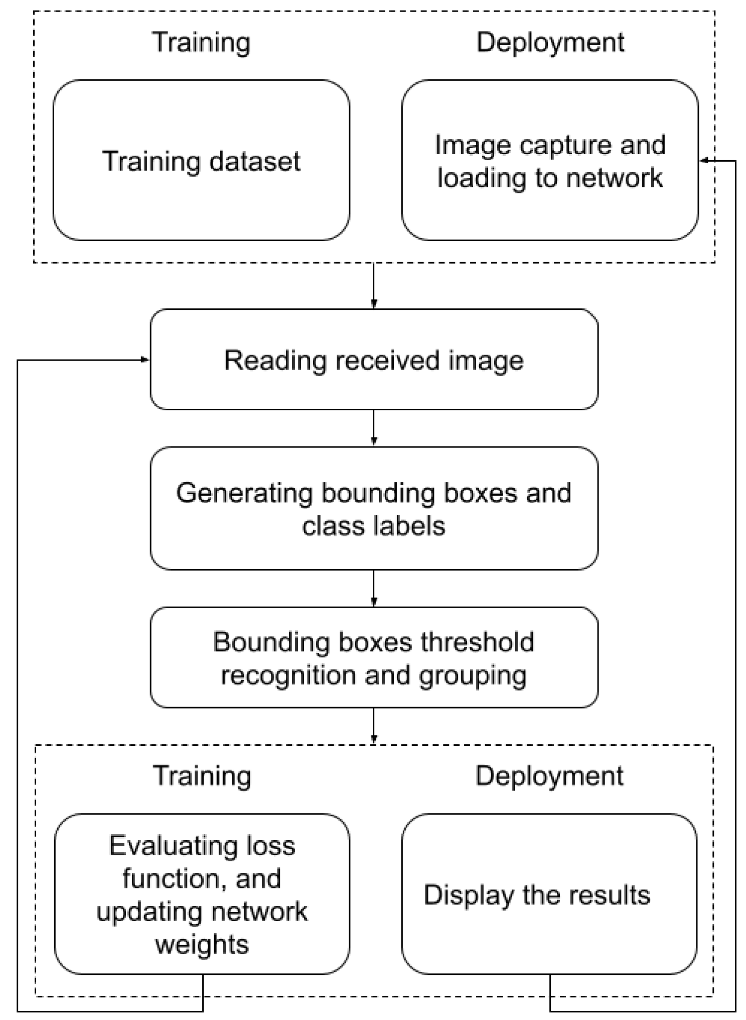
The proposed system is capable of detecting and counting surface-mounted devices (SMDs) on a conveyor. For this task, we needed a dataset with images such as SMD components. Several available datasets offer only images of SMD components on a PCB. Therefore, to train the investigated algorithms, an SMD-type component dataset was collected on a conveyor belt. The system is composed of a hardware computing unit with a camera and a mechanical system—a conveyor belt on which components are moving. The hardware unit is responsible for the real-time identification and detection of the electronic SMD components on the conveyor. The system workflow diagram is shown in Figure 1. It is assumed that the desired model is loaded into the system. The images of the SMD components are captured while they move on a conveyor. In the images obtained, the bounding box and the type of SMD components are displayed as an output of the system. The most challenging part is a successful identification of components in real-time. In the remainder of this section, we will describe the details of the proposed approach.

2.1. Hardware Setup

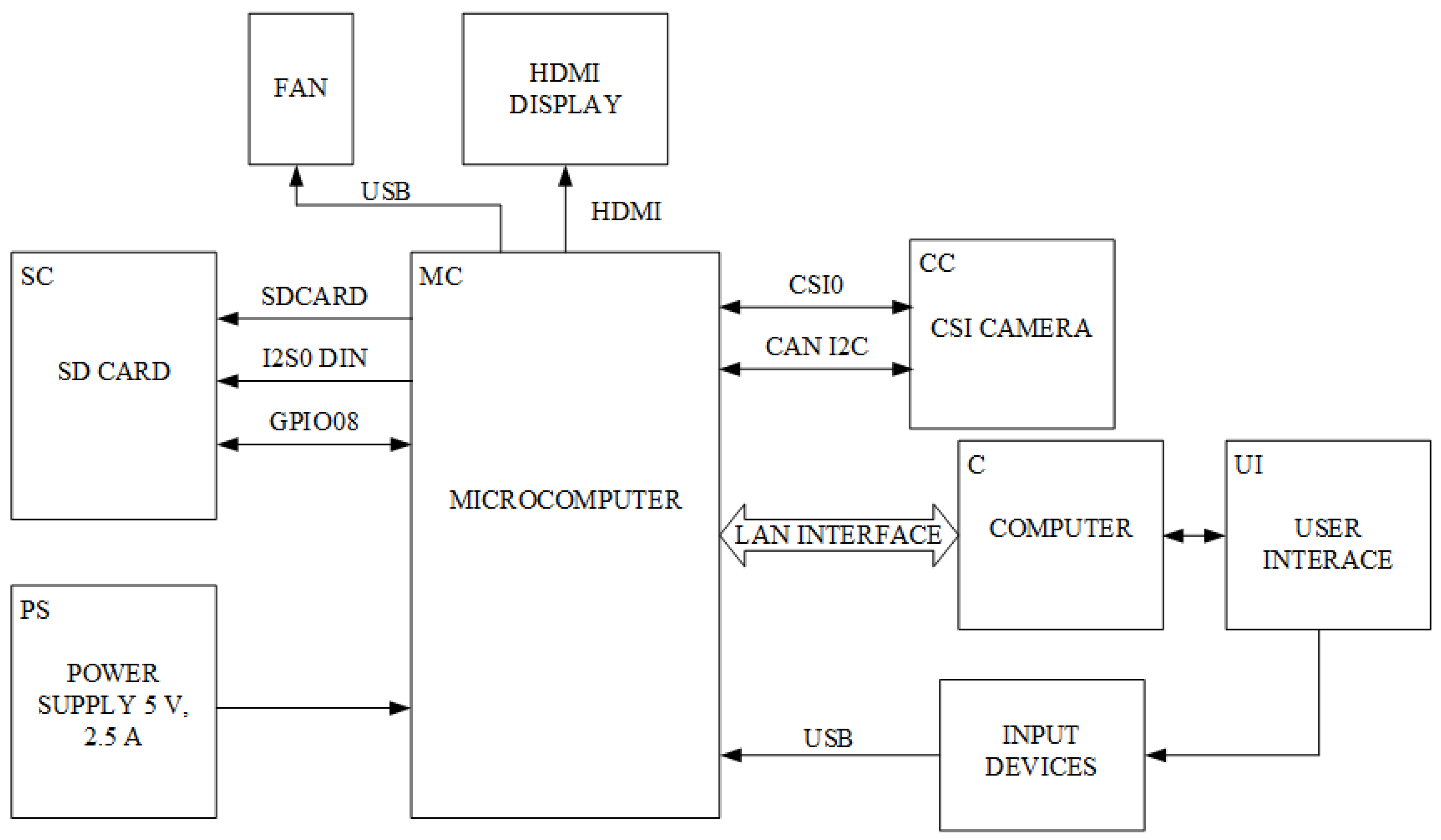
The hardware setup designed for the detection and counting of electronic components is shown in Figure 2. The system was designed to be inexpensive and meet the requirements of real-time detection in an industrial environment. The microcomputer was powered by a general power source. A camera was connected to the microcomputer for video input and an HDMI-connected screen was used to display results. SD memory was connected to store data and software for object detection. The user controls the microcomputer through the LAN interface and input devices. Additionally, a ventilator was connected to cool the microcomputer.

For the hardware setup described, an Nvidia Jetson Nano microcomputer was chosen [63]. It has a 128-core Maxwell GPU, 4-core ARM A57 CPU, 4 GB LPDDR4 memory, HDMI and display connectors, USB, and other interfaces. To capture moving objects, a Raspberry Pi NoIR Camera v2 CSI camera was connected [64]. The camera has an 8-megapixel sensor and supports 1080p30 and 720p60 video formats. SD card size was 64 GB. SD card containing a dataset and data for training epochs. Power supplied by micro-USB T6712DV. The user interface was communicated through the LAN, using VNC Server software. Additionally, for customization, a mouse and keyboard were connected via USB. Ventilator power was 2.5 W, which was supplied by USB from the microcomputer.

Nvidia Jetson Nano microcomputer was chosen because of its ratio between price and performance. The device can implement the currently available deep learning algorithms. Moreover, the device supports Nvidia JetPack, which included board supports package, Linux OS, CUDA, cuDNN, and TensorRT deep learning libraries, dedicated for object detection. Additionally, the device has many input and output ports, power is supplied through USB, and has various interfaces, such as GPIO, CSI.

The Raspberry Pi Noir CSI camera was connected to the microcomputer. The camera has a high-quality 8 megapixel Sony IMX219 image sensor, which is capable of working with various illuminance conditions. The camera is capable of capturing 3280 × 2464 px static images, and also supports 1080p30, 720p60 and 640 × 480p90 video modes [64]. The small size and light weight of the camera module allow it to be easily mounted on the conveyor. In case of low illuminence, the No Infrared lens filter allows one to capture high-quality images.

During the testing phase of our hardware setup, high temperatures (beyond 65 °C) of the microcomputer were observed. To maintain the working temperature of the CPU and GPU, an external 2.5 W ventilator was connected. The size of the ventilator was 160 × 150 × 100 mm, with a 5 V USB power supply. With the connected ventilator, the temperature of the system did not rise above 35 °C. For stable illuminence, a 4400 K color and 6600 lm brightness was used.

2.2. Dataset Collection and Augmentation

The dataset was collected using Nvidia Data Capture Control [65]. This SDK allows the collection and labelling of the data stream from the camera in real time. The tool allows several settings, such as simplified labeling of data for classification and detection, to easily distribute data to the training, validation, and test sets.

The dataset consists of images of SMD-type electronic components, which are moving on a conveyor belt. There are four types of components in the collected dataset:

• Capacitors;
• Resistors;
• Diodes;
• Transistors.

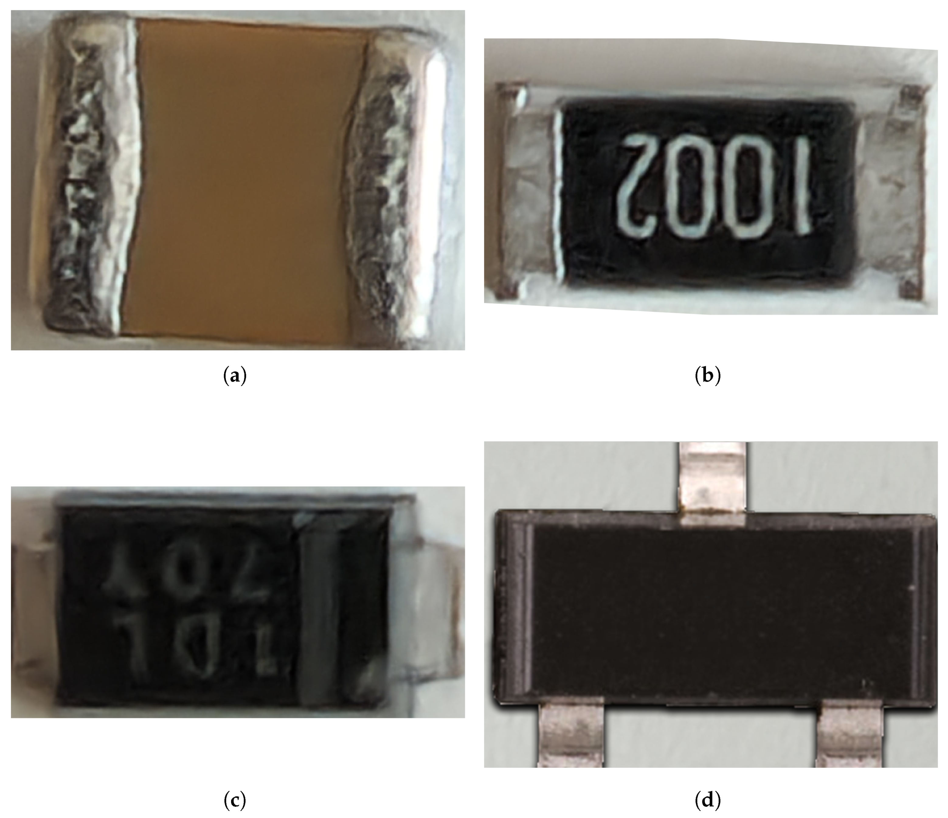
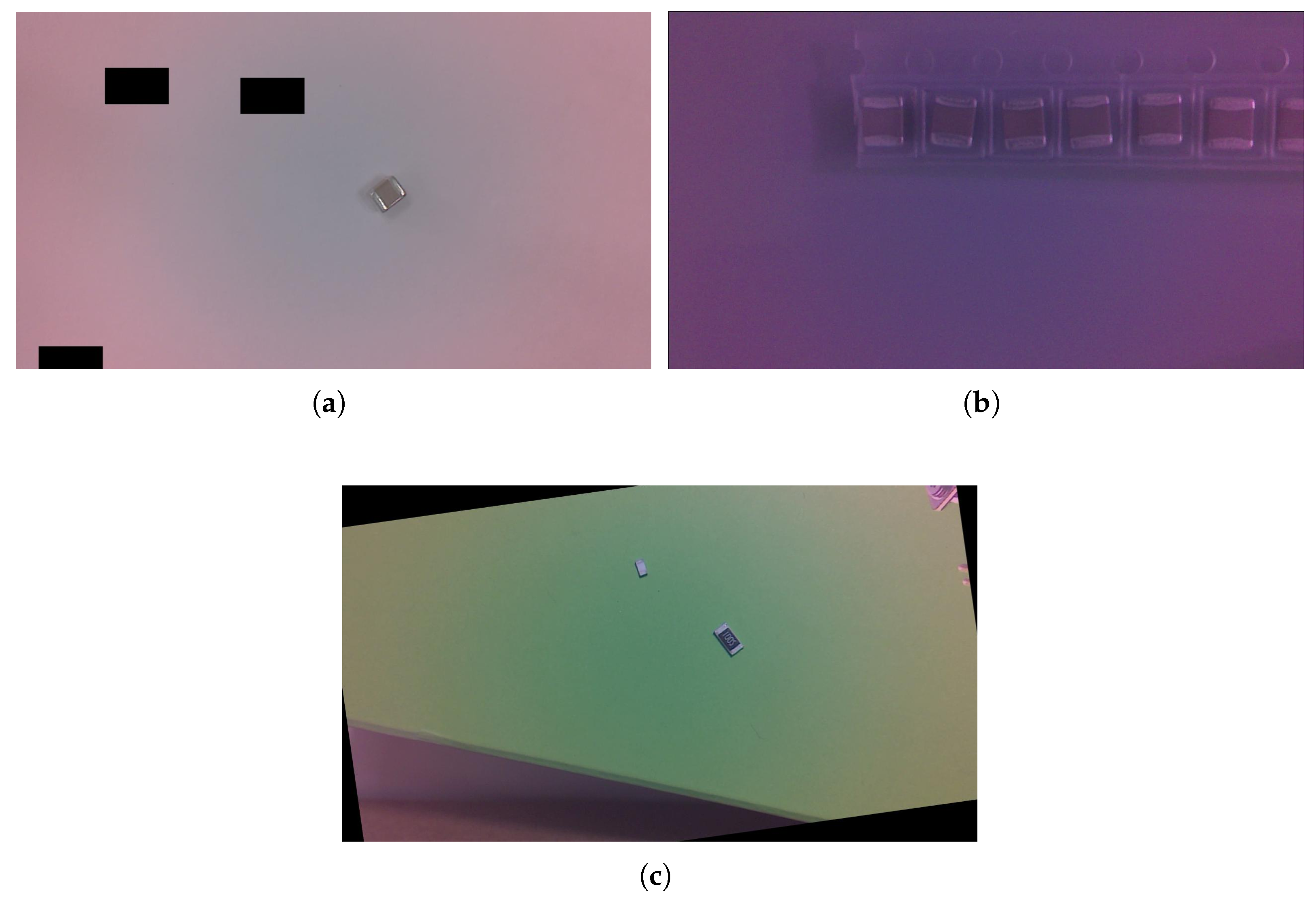
Illustrations of these components are shown in Figure 3. These components were chosen because of their popularity, quantity, form of packing (most of the time SMD components are packed in bulk), and difficulty to detect. For example, a capacitor (Figure 3a) can be visually identified by soldering silver-colored joints on the left and right sides, which cover the middle area of the ceramic with a light-brown color. As seen in Figure 3, SMD components, used in our work, are difficult to distinguish between. The key to distinguishing these components is their silver-colored solder joints. Resistors’ solder joints look similar to capacitors, diodes are similar as well, but thinner compared to resistors. Transistors have three small solder joints. Other key features are that resistor body area only includes a number, while a diode additionally has a letter, a thin gray or white stripe, which is drawn from top to middle. A transistor can include numbers and letters on its body. However, these printouts are not certain; some manufacturers do not include any identification prints. For this reason, the task of identifying the SMD components is difficult.

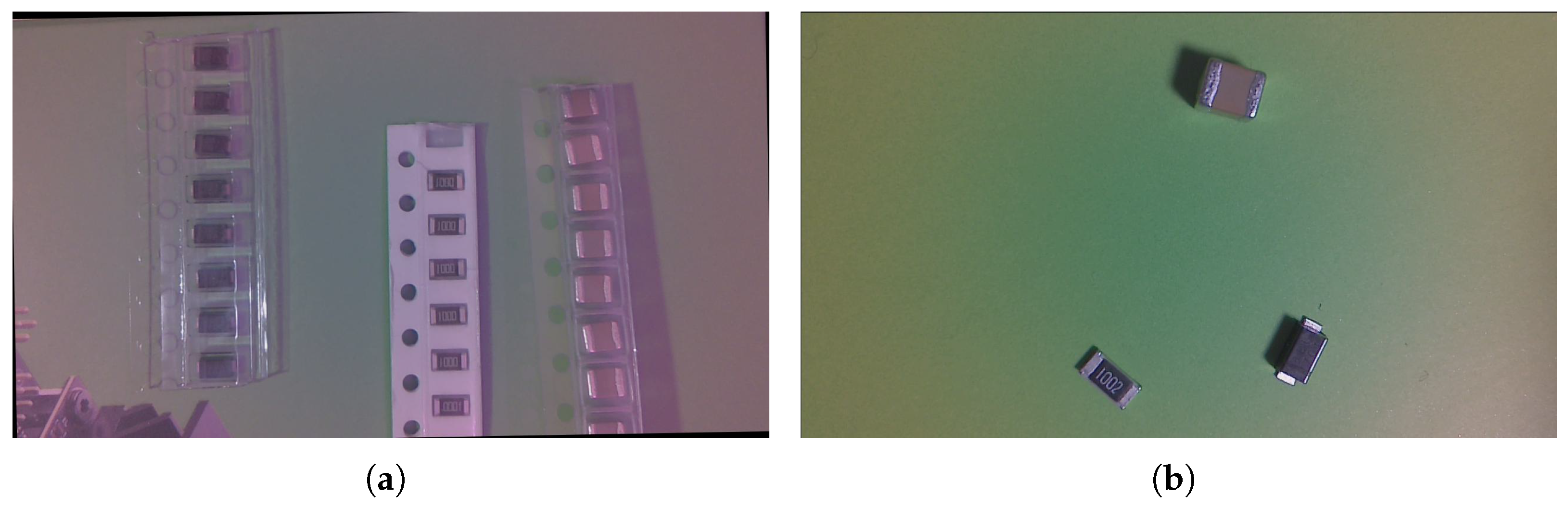
Another challenge is the unknown number and type of packing of the components. Components on the conveyor are placed separately or in a package. In the collected dataset, we have used images containing single, multiple unpacked, and multiple packed components. The number of components was not labeled for training, but ranged from 1 to 30. In this way, the investigated models were trained to identify an unknown number of differently packed components. An illustration of the packing style and multiple components is shown in Figure 4.

For the initial dataset, we collected 3005 images. The dataset was divided to 2405 images for training, 300 images for validation and test sets. The images were divided by random sampling. In total, 11,875 annotated components were in the dataset, which consists of 3297 capacitors, 4478 resistors, 3404 diodes and 696 transistors. The initial dataset was used to test various conditions of our system, such as illuminence, angle of the camera, and quality of images. Object-detection algorithms were also tested using this dataset.

After confirming the proper conditions of our system, an initial dataset was expanded using data augmentation. The data were preprocessed to automatically reorient pixels (removing EXIF orientation). An example of image augmentation is shown in Figure 5. The data augmentation techniques that we used for the dataset were random cutouts, color augmentation, rotation. These techniques were chosen because of their inability to hide small features of electronic components. Random cutouts (shown in Figure 5a) are similar to the size of SMD components and are intended to increase the robustness of trained models. Soldering leads are the primary visual cue to distinguish SMD components. Therefore, other augmentation methods, such as brightness or contrast adjustment, which assimilate the leads and background, were not used for augmentation. Color augmentation (shown in Figure 5b) adjusts input image hue property, which randomly alters the color channels, causing a model to use alternative color schemes.

After data augmentation, the dataset consisted of 4061 images—3429 for training, 406 for testing and validation—with 15,950 annotated components: 6007 resistors, 4581 diodes, 4470 capacitors, and 892 transistors. Later dataset was augmented using scaling and rotation (90°, random between −15° and +15°, as shown in Figure 5c). The final dataset consisted of 7661 images, which were divided, using random sampling, into 7061 images for the training set, 300 images for the test set, and 300 images for the validation set. The final dataset consisted of 28,536 annotated SMD components:

• 8198 capacitors;
• 10,467 resistors;
• 8543 diodes;
• 1328 transistors.

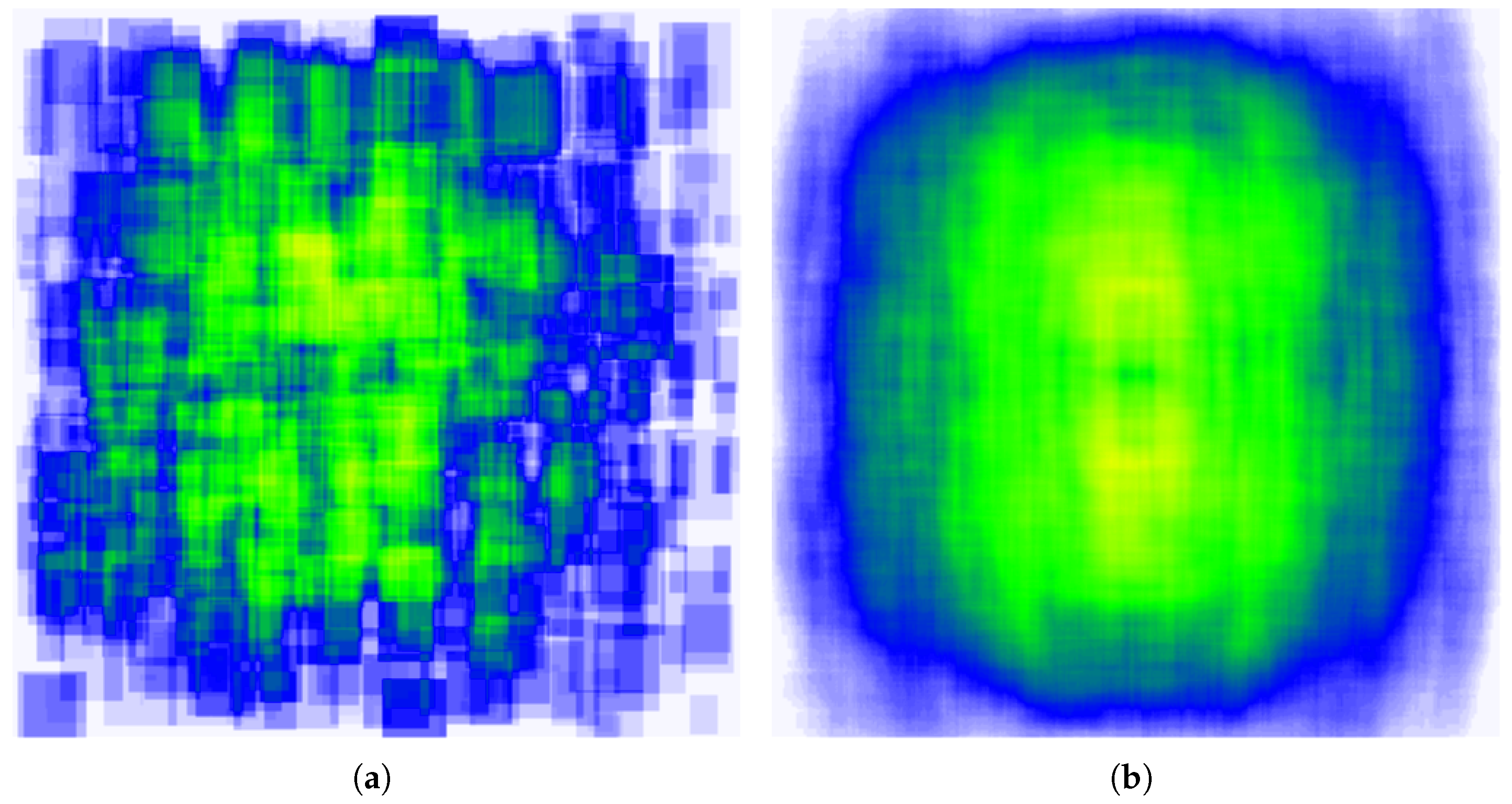
Additionally, in the dataset, non-relevant objects that had similar color palettes and shapes as the SMD components were included. Furthermore, the illumination conditions and angle of the camera were adjusted to induce possible data variations of real-life conditions, such as dust or the appearance of an accidental unknown object. In Figure 6, an annotation location map for the dataset is shown. Most components are shown to be located in the center of the image (yellow, green color).

Dataset was collected using Pascal VOC format, and eventually converted to COCO, darknet, YOLO-keras, YOLO-V4 PyTorch, YOLO-V5 PyTorch formats. The image resolution in the dataset is 1280 × 720 px and file size is between 26–40 KB. To export data to different formats, RoboFlow [66] was used. Different formats were used to test the performance of different implementations of deep learning algorithms.

2.3. Training of Models

In this work, we implemented and investigated SSD-Mobilenet-v1, YOLO-V3, YOLO Scaled-YOLO-V4, YOLO-V4, YOLO-V5 algorithms. Training algorithms were implemented using the PyTorch and Keras libraries. Additionally, reduced network architectures were trained to investigate the performance of the designed hardware. All the investigated algorithms were trained using AMD Ryzen 5 5800H CPU, Nvidia Geforce RTX 3060 GPU, and Google Colab service with Tesla P100-16 GB GPU.

The models were trained using our collected dataset. Initially, we used pre-trained models. The number of iterations and epochs were kept identical for all trained architectures. The training methodology was based on [67,68]. The size of the trained models and libraries used are given in

Table 1. Size and libraries used for the trained algorithms.

Model	Library	Model Size, MB
SSD-MobileNet-v1	PyTorch	36.2
YOLOv3	Keras	237.2
YOLOv3-tiny		33.9
YOLOv4	Darknet	244.2
YOLOv4-tiny		22.5
YOLOv4-Scaled	PyTorch	401.3
YOLOv5s		14.1

.

The first model we investigated was a regression-based SSD-Mobilenet-v1 algorithm. SSD-300 and Mobilenet detector were used [69]. This algorithm is frequently implemented on smartphones and integrated devices for real-time applications of various object-detection problems. In our experiment, a pre-trained mobilenet-v1-ssd-mp-0.675 model was used. The model was loaded using PyTorch library functions and trained on the collected dataset. The model was trained for 100 epochs. The training results showed a validation loss of 2.1466. The size of the trained model was 36.2 MB.

Several YOLO algorithms were investigated in our experiment, such as YOLOv3, YOLOv3-tiny, YOLOv4, YOLOv4-tiny, YOLOv4-Scaled, and YOLOv5s. For the input of the algorithms, 416 × 416 px size images were used. The main differences between all YOLO algorithms were the backbone of the network: YOLOv3 uses Darknet53, YOLOv4 uses the CSPdarknet53 backbone, and YOLOv5 uses the Focus structure with the CSPdarknet53 backbone [70].

YOLOv3 and YOLOv3-tiny models were configured and trained using the Keras library [71]. Both models were trained for 100 epochs using Layers freeze. YOLOv3 model validation loss was 12.607, and size was 237.2 MB. The YOLOv3 tiny model training was stopped when validation loss was 11.642, the model file size was 33.9 MB.

Darknet library was used to train YOLOv4 and YOLOv4-tiny models [72]. The models were trained for 8000 batch iterations. Final size of the YOLOv4 model was 244.2 MB, and of the YOLOv4-tiny—22.5 MB.

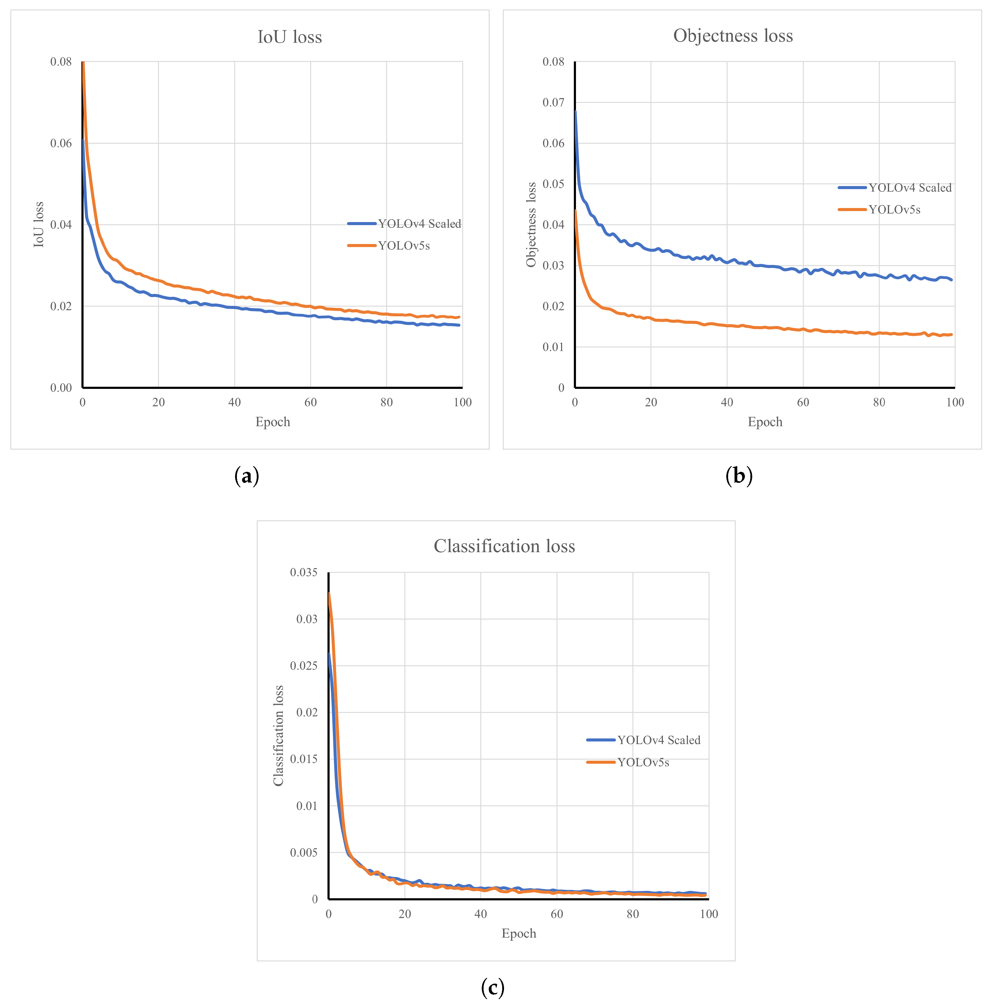
Furthermore, to train and adopt the YOLOv4-Scaled and YOLOv5s models, the PyTorch library was used. The models were trained for 100 epochs and the model sizes were 401.3 and 14.1 MB, respectively. A detailed training diagram is given in Figure 7. In the given figure, Intersection over Union (IoU), objectness and classification losses are shown. The loss of IoU shows how well the algorithms investigated can detect the center and edges of the components. Based on the results shown, YOLOv4-Scaled achieved a lower IoU loss after training for 100 epochs. Objectness loss shows the probability to find the object in the detect square box. It is shown that YOLOv5s achieved better objectness by approx. 0.014 points. Classification loss shows how well the algorithm can assign a correct label to the detected objects. Based on the results shown, both algorithms displayed similar results.

2.4. Evaluation Criteria

In the experimental research, several evaluation metrics were used and implemented, as described in [73,74]. An average precision (AP) score was calculated for each SMD component, and mean AP (mAP) score was used to assess the performance of the system to detect the four components [73]. IoU threshold was set to 0.75. 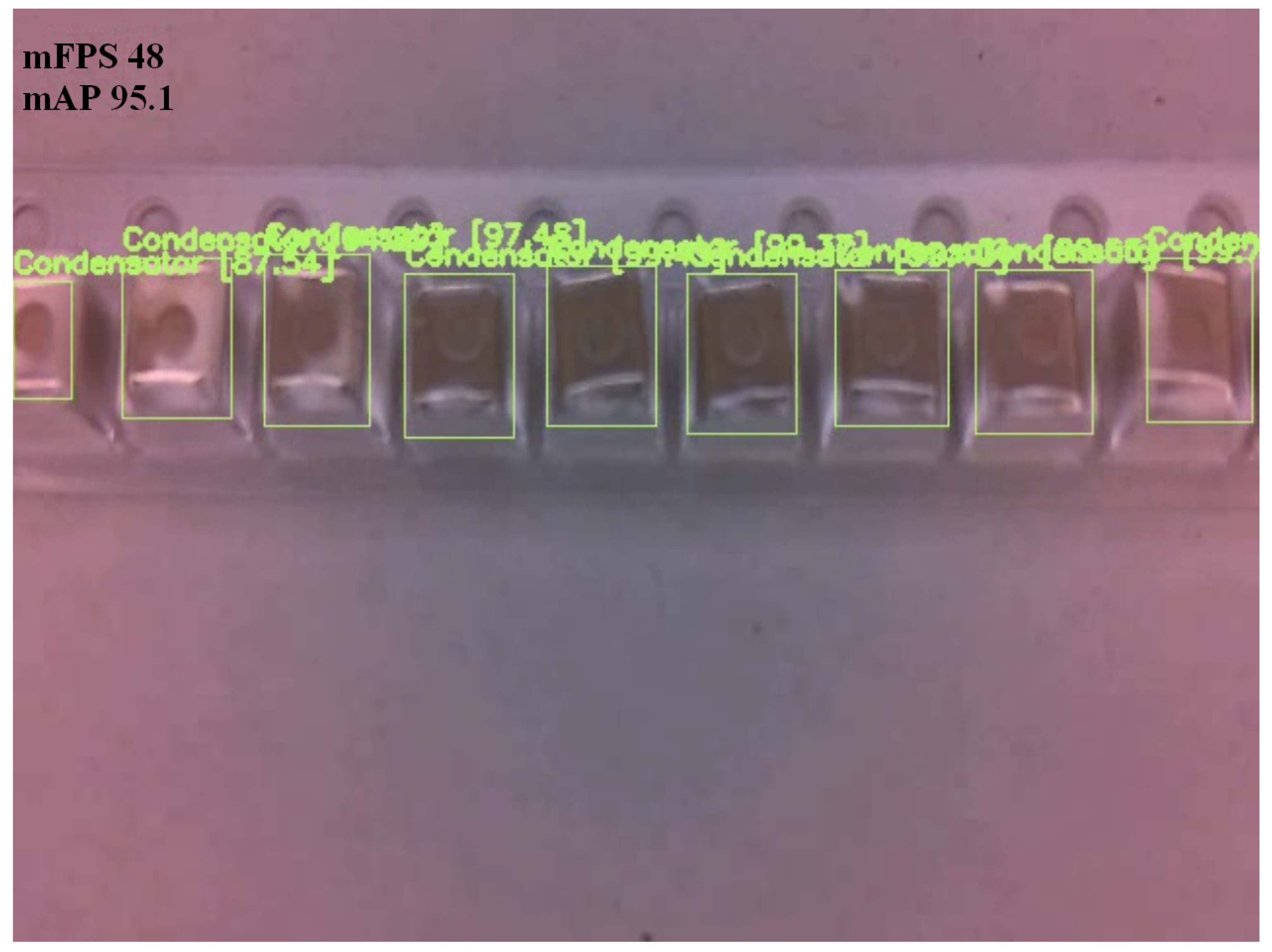Additionally, to evaluate the speed with which implemented architectures can detect objects, the architectures were compared by the speed of frames processed per second (FPS) and Inference Time (IT) [74]. Experimental results were obtained using Google Colab with Tesla P100-16 GB and Nvidia Jetson Nano 4 GB hardware setup. A sample image of successfully detected capacitors, moving in a line as packed components, on a conveyor belt, is shown in Figure 8. Components in the image were detected using the YOLOv4 architecture.

3. Experimental Results

In Section 2, the implementation of the integrated system for the SMD component detector was described on a conveyor capable of running several state-of-the-art deep learning algorithms. In addition, we describe the collected data set and the training of the models. Using the proposed hardware setup, we conducted experimental research to find the limitations of the IT and mAP scores with various implementations of deep learning algorithms, when counting SMD components on a conveyor.

The experimental results of the deep learning algorithms implemented in the proposed hardware, when detecting capacitors, are given in

Table 2. Experimental results of investigated deep learning algorithm implementations for capacitor detection.

	Tesla P100-16 GB			Jetson Nano 4 GB
Model	AP, %	FPS	IT, ms	AP, %	FPS	IT, ms
SSD-Mobilenet-V1	66.7	89	11.2	66.6	42	23.8
YOLOv3-Keras	90.2	14	71.4	90.1	1	1000
YOLOv3-tiny	83.1	19	52.6	82.7	4	250
YOLOv4	94.4	49	20.4	94.6	1	1000
YOLOv4-tiny	97.3	96	10.4	97.3	18	55.6
YOLOv4-Scaled	87.8	44	22.7	86.7	4	250
YOLOv5s	88.6	89	11.2	85.3	8	125

. As the results show, the highest AP score was displayed by the YOLOv4-tiny algorithm—97.3%—using both hardware setups. In general, the average precision between two hardware setups was less than 0.5% for the SSD-Mobilenet-V1, YOLOv3-Keras, YOLOv3-tiny, YOLOv4 and YOLOv4-tiny architectures. Tesla P100 compared to Jetson Nano showed higher AP by 1.1%, 3.3% for the YOLOv4-Scaled and YOLOv5s architectures, respectively. The inference times were different by magnitudes from 2 to 50, depending on the investigated algorithm. Lowest IT, of 10.4 ms was found for the YOLOv4 tiny algorithm when using Tesla P100 setup, and 23.8 ms for SSD-Mobilenet-V1 algorithms (AP was 66.6%) when using the Jetson Nano setup.

The experimental results of the deep learning algorithms on the proposed hardware, when detecting resistors, are given in

Table 3. Experimental results of investigated deep learning algorithm implementations for resistor detection.

	Tesla P100-16 GB			Jetson Nano 4 GB
Model	AP, %	FPS	IT, ms	AP, %	FPS	IT, ms
SSD-Mobilenet-V1	75	89	11.2	75.1	41	24.4
YOLOv3-Keras	92.7	15	66.7	92.7	1	1000
YOLOv3-tiny	76.3	18	55.6	65.2	6	166.7
YOLOv4	97.7	48	20.8	98.6	1	1000
YOLOv4-tiny	98.5	92	10.9	98.5	18	55.6
YOLOv4-Scaled	89.1	44	22.7	89.1	2	500
YOLOv5s	92.9	70	14.3	91	8	125

. As the results show, the highest AP was found using the YOLOv4 algorithm, 98.6% with the Jetson Nano hardware setup, and 98.5% using YOLOv4-tiny on Tesla P100. In general, the average precision between two hardware setups was less than 1% for SSD-Mobilenet-V1, YOLOv3-Keras, YOLOv4, YOLOv4-tiny, and YOLOv4-Scaled architectures, while Tesla P100 showed higher AP by 11.1% when using YOLOv3-tiny architecture and higher by 1.9% when using YOLOv5s architecture, compared to Jetson Nano. The inference times were different by magnitudes from 2 to 20, depending on the algorithm investigated. The lowest IT—10.9 ms—was found when investigating the YOLOv4 tiny algorithm using the Tesla P100 setup, and 24.4 ms for SSD-Mobilenet-V1 algorithms (AP was 75.1%) when using Jetson Nano setup.

Experimental results of deep learning algorithms implemented on the proposed hardware, when detecting diodes, are given in

Table 4. Experimental results of investigated deep learning algorithm implementations for diode detection.

	Tesla P100-16 GB			Jetson Nano 4 GB
Model	AP, %	FPS	IT, ms	AP, %	FPS	IT, ms
SSD-Mobilenet-V1	67.3	92	10.9	67.2	41	24.4
YOLOv3-Keras	88.6	16	62.5	88.7	1	1000
YOLOv3-tiny	65.3	21	47.6	65.2	6	166.7
YOLOv4	66.2	49	20.4	85.9	1	1000
YOLOv4-tiny	76.2	122	8.2	76.5	18	55.6
YOLOv4-Scaled	70.7	46	21.7	70	2	500
YOLOv5s	82.8	79	12.7	81.2	8	125

. As the results show, the highest AP score was displayed by the YOLOv3-Keras algorithm—88.6% and 88.7% using Tesla P100 and Jetson Nano hardware setups, respectively. In general, the AP between two hardware setups was less than 1% for SSD-Mobilenet-V1, YOLOv3-Keras, YOLOv3-tiny, YOLOv4-tiny, and YOLOv4-Scaled algorithm implementations. Tesla P100 hardware setup, compared to Jetson Nano, showed a lower AP by 19.7% when the YOLOv4 algorithm was implemented and a higher AP by 1.2% when the YOLOv5 algorithm was implemented. The inference times were different by magnitudes from 2 to 50, depending on the investigated algorithm. The lowest IT—8.2 ms—was found for YOLOv4-tiny algorithm implementation when using Tesla P100 setup, and 24.4 ms for SSD-Mobilenet-V1 algorithms (AP was 67.2%) when using the Jetson Nano setup.

The experimental results of the deep learning algorithms implemented on the proposed hardware, when detecting transistors, are given in

Table 5. Experimental results of investigated deep learning algorithm implementations for transistor detection.

	Tesla P100-16 GB			Jetson Nano 4 GB
Model	AP, %	FPS	IT, ms	AP, %	FPS	IT, ms
SSD-Mobilenet-V1	60.6	89	11.2	60.5	36	27.8
YOLOv3-Keras	66.9	15	66.7	66.9	1	1000
YOLOv3-tiny	63.5	19	52.6	63.5	6	166.7
YOLOv4	95.4	46	21.7	97.2	1	1000
YOLOv4-tiny	79.9	65	15.4	79.8	17	58.8
YOLOv4-Scaled	69.6	41	24.4	69.5	2	500
YOLOv5s	68.8	91	11	70.6	8	125

. As the results show, the highest AP score was displayed by the YOLOv4 algorithm—95.4% and 97.2% for both hardware setups. In general, the AP between two hardware setups was less than 1% for SSD-Mobilenet-V1, YOLOv3-Keras, YOLOv3-tiny, YOLOv4-tiny, YOLOv4-Scaled and YOLOv5s algorithm implementations. Tesla P100 hardware setup, compared to Jetson Nano, showed a lower AP of 1.8% when YOLOv4 and YOLOv5s algorithms were implemented. The inference times were different by magnitudes from 2 to 50, depending on the algorithm investigated. The lowest IT—11 ms—was found when using the YOLOv5s algorithm (AP was 68.8%) on the Tesla P100 setup, and 27.8 ms when using SSD-Mobilenet-V1 algorithm (AP was 60.5%) on the Jetson Nano setup.

The experimental results of deep learning algorithms implemented on the proposed hardware, when detecting all four components, are given in

Table 6. Experimental results of investigated deep learning algorithm implementations for detection of capacitor, resistor, diode and transistor SMD components.

	Tesla P100-16 GB			Jetson Nano 4 GB
Model	AP, %	FPS	IT, ms	AP, %	FPS	IT, ms
SSD-Mobilenet-V1	67.4	89.75	11.1	67.35	40	25.1
YOLOv3-Keras	84.6	15	66.8	84.6	1	1000
YOLOv3-tiny	72.05	19.25	52.1	69.15	5.5	187.5
YOLOv4	88.43	48	20.8	94.08	1	1000
YOLOv4-tiny	87.98	93.75	11.2	88.03	17.75	56.4
YOLOv4-Scaled	79.3	43.75	22.9	78.83	2.5	437.5
YOLOv5s	83.28	82.25	12.3	82.03	8	125

. As the results show, the highest mAP score of 94.08% was demonstrated using the implementation of the YOLOv4 algorithm on Jetson Nano with an inference time of 1000 ms. Furthermore, the YOLOv4 model showed 88.433% mAP on the Tesla P100 with IT of 20.8 ms. The second-highest mAP score was found using the Jetson Nano hardware setup with implementation of the YOLOv4 algorithm; it was 88.03%, and IT was 56.4 ms, and a 87.98% mAP score with 11.2 ms using Tesla P100 platform was observed. The differences in mAP between the hardware setups of the implementations of the SSD-Mobilenet-V1, YOLOv3-Keras, YOLOv4-tiny, YOLOv4-Scaled, and YOLOv5s algorithms were less than 1.25%. Higher mAP differences were found using the YOLOv3-tiny and YOLOv4 algorithms; these were higher by 2.9% and 9.15% when comparing the Tesla P100 hardware setup with the Jetson Nano. Inference time of SSD-Mobilenet-V1 was one of the lowest—11.1 and 25.1 ms for Tesla P100 and Jetson Nano hardware setups, respectively. However, the mAP scores of the SSD-Mobilenet-V1 algorithm were 67.4% and 67.35% for Tesla P100 and Jetson Nano setups, respectively.

4. Discussion

The highest mAP score under 70 ms IT for all components was achieved using the YOLOv4-tiny algorithm on a Jetson Nano platform: 88.03% mAP. Naturally, a larger YOLOv4 network showed a higher mAP score of 94.08% mAP, but at IT of 1000 ms. Our experimental results are in line with similar research [75]. The authors of this paper implemented and investigated the performance of several deep learning algorithms (including YOLOv4 and YOLOv4-tiny) for an electronic component conveyor belt. Their findings show that YOLOv4-tiny achieves slightly higher mAP. However, the hardware and mounting type of electronic components were different from our work. In their research (compared to ours), the authors used a more powerful hardware system, with an Intel Core i7-8700 CPU, NVIDIA TITAN Xp GPU, 32 GB RAM. In addition, the authors intend to deploy their proposed method on an embedded computing device in their future work. Furthermore, the detected electronic components were of through-hole technology type, which is visually much easier to distinguish; in particular, differences between resistors and capacitors are clearly identifiable. In another work [60], the results of the experimental research showed that YOLOv4 architectures achieve a higher mAP score compared to YOLOv3 when detecting SMD components on a PCB board. However, the hardware used in this investigation is not reported.

The detection of electronic components on the conveyor did not reach 100%, due to the three main challenges of the problem. The first is the difficulty of distinguishing the SMD components from one another; the main differences between the components are the size and shape of the leads. The second challenge is to meet the requirements of real-time detection: while we run a real-time detection, the conveyor moves and changes its velocity. Thus, it adds noise to the input image (e.g., blur, unwanted reflections from lightning). Such noises introduce distortions and make it difficult to distinguish components that already have small visual differences. The third challenge is the requirement that the model is able to operate in the embedded computing device. Such devices usually have limited computing power and are required to operate in real-time. In practice, it is a common setup to reduce deployment and scaling costs. Thus, these three challenges decrease the performance of the detector.

In our work, we investigated the detection of four different electronic components, these being capacitors, resistors, diodes, and transistors. In practice, resistors and capacitors contribute to the largest volume of electronic components on a conveyor. The average precision for the detection of capacitors and resistors was 97.3% and 97.7%, respectively. Several recently published research papers accentuate the challenge of detecting these two components with a higher that 96% mAP [47,58,76]. Our results show a considerable improvement in the detection of resistors and capacitors.

To deploy a deep learning algorithm in a real-time object detection system, one needs to choose an algorithm that can process a certain number of images per second. In practice, FPSs above 15 are sufficient when detecting and counting SMD components on a conveyor (or inference time below 70 ms). Similar research works, proposing the automatic identification of electronic components, deploy their system on powerful graphical processors including NVIDIA TITAN Xp GPU [75], NVIDIA Quadro P5000 [58], NVIDIA GTX 1050 [53]. On the contrary, our proposed system setup includes a microcomputer running on an embedded device. Based on our results, the Tesla P100 platform achieved the desired inference time for all models investigated. However, considering scale, price and performance ratio, a more realistic approach would be to deploy such a system on a Jetson Nano microcomputer. In this case, only several algorithms achieved mAP above 90%, with ITs below 70 ms. Our results show that YOLOv4-tiny is the best choice to implement in an integrated system with a Jetson Nano microcomputer when detecting four types of SMD components; when detecting capacitors, the algorithm achieves 97.3% AP at 55.6 ms IT; when detecting resistors, the algorithm achieves 98.5% AP at 55.6 ms IT.

Based on the experimental results, we can see that Tesla P100 detects objects at higher FPS. One way to speed up the FPS for the Jetson Nano would be pruning technique. In our work, we avoided using pruning of the models. Instead, we investigated the performance of deploy-ready models, such as YOLOv4-tiny, SSD-Mobilenet-V1, YOLOv3-tiny, YOLOv5s. Therefore, a trade-off between IT and mAP can be noticed when comparing pruned models with their counterparts (e.g., YOLOv4 and YOLOv4-tiny), which is the expected outcome, since reducing the size of model improves the IT and reduces the mAP. However, when comparing similarly sized, but different architectures (e.g., SSD-MobileNet-V1 and YOLOv3-Keras) a trade-off between IT and mAP was not found.

In theory, deployed models should achieve similar AP scores regardless of the hardware they are deployed with. However, our results show that several algorithms, such as YOLOv3-tiny, YOLOv4 achieve different AP scores based on the hardware they are deployed with. Such dependencies may arise from custom hardware-based neural network accelerators [77]. However, future research directions should not only aim to improve the AP and IT scores in case of real-time SMD component detection, but also investigate the dependencies of the AP score based on the deployed platform.

5. Conclusions

In this study, a real-time integrated SMD component detection and classification system with a camera and a CNN deep learning model was proposed. In addition, in this work, we provide a performance comparison of several CNN deep learning models deployed in the system. The performance of the algorithms investigated was compared using mean average precision and inference time. The proposed hardware setup shows how to build a low-cost integrated system for a conveyor in order to detect packed and unpacked moving SMD components. The system meets the requirements for real-time detection in an industrial environment with all limitations. Experimental results were obtained using the dataset containing 7061 images of 8198 capacitors, 10,467 resistors, 8543 diodes, 1328 transistors. Based on the results of this study, we can conclude that:

• Proposed system includes a hardware setup with a camera and an implemented CNN deep learning model, and meets the requirements of real-time detection and counting of SMD components on a conveyor belt;
• When detecting SMD-type capacitors on a conveyor, the highest mAP of 97.3% was achieved using YOLOv4-tiny algorithm implementation on the Tesla P100-16 GB and Jetson Nano 4 GB microcomputers;
• When detecting SMD-type resistors and transistors, the highest mAPs of 97.7% and 98.6% (for resistors) and 95.4% and 97.2% (for transistors) were achieved using YOLOv4 algorithm implementation on Tesla P100-16 GB and Jetson Nano 4 GB microcomputers, respectively;
• When detecting SMD-type diodes, the highest mAP of 88.6% and 88.7% was achieved using YOLOv3-Keras algorithm implementation;
• When detecting four types of SMD components on a conveyor, the highest mAP using an Nvidia Jetson Nano 4 GB microcomputer was achieved with the YOLOv4 algorithm, which is 94.08% with 1000 ms IT; using the YOLOv4-tiny algorithm on a Jetson Nano 4 GB microcomputer, IT is 56.4 ms, with an mAP score of 88.03%;
• When detecting four types of SMD components on a conveyor, the highest mAP using Google Colab’s Tesla P100-16 GB was achieved with the YOLOv4 algorithm, which is 88.43% with 20.8 ms IT.